76
ANALYSIS OF FINANCIAL MANAGEMENT AND WORKING
CAPITAL BY USING DIFFERENT ANALYSIS RATIO
Author name: Repalle Vinod Department: Management
ABSTRACT
Efficient Management of Working capital is one of the preconditions for success of an organization as Working Capital is the life giving force to an economic entity. Efficient management of working capital means management of various components of working capital in such a way that an adequate amount of working capital is maintained for smooth running of a firm and for fulfillment of twin objectives of liquidity and profitability. Also it is the most crucial factor for survival and solvency of a concern. While inadequate amount of working capital impairs the firm's liquidity, holding of excess working capital results in the reduction of the profitability. But the proper estimation of working capital actually required, is a difficult task for the management because the amount of working capital varies across firms over the periods depending upon the nature of business, scale of operation, production cycle, credit policy, availability of raw materials, etc. This paper analysis the working capital profitability position by using different profitability ratio tools and One Way ANOVA for selected companies. Varieties of ratio analysis are used here to find the exact result on profitability of a company. It involves in-depth analysis of profitability of the company with the help of key ratios, statistical analysis and growth chart in terms of turnover & profit.
KEYWORDS: working capital, Liquidity, Profitability, ANOVA.
I-INTRODUCTION
Profitability ratios help in ascertaining the position of the company with respect to various profitability measures like Operating Profit, Net Profit & Return on Net Worth. Comparative study of annual increase in sales and profitability is made to understand the growth of the company. Conclusions are drawn with the help of results obtained through aforesaid techniques.
II-OBJECTIVES
1. Analysis of varieties of ratios to ascertain the working capital effects on selected companies.
III METHODOLOGY
Research methodology is a way to systematically solve the research problem. It may be understood as a science of studying now research is done systematically.
Data collection plays an important role in research work. Without proper data available for analysis you cannot do the research work accurately.
There are two types of data collection methods available. a. Primary data collection
b. Secondary data collection 3.1 Data analysis
After collection of the data the second step is analyze the data. In this report we use the Profitability Ratio (Return on Investment) and working capital Ratio. We compare both ratios with the Karl Pearson’s correlation co-efficient statistical tool. With the help of primary data and mainly secondary data we could found the below results.
No. of Days A/R = (Accounts Receivables/Sales) x 365
No. of Days A/P = (Accounts Payables/Cost of Goods Sold) x 365
No. of Days Inventory = (Inventory/Cost of Goods Sold) x 365
Cash Conversion Cycle = (No. of Days A/R + No. of Days Inventory) – No. of Days A/P
Financial Debt Ratio = Short term loans + long term loans/total assets
Fixed Financial Asset Ratio = Fixed Financial Assets/Total assets
Profit = (Sales - Cost of Goods Sold) / (Total Assets - Financial Assets)
77
operating activity that might affect overall profitability. Therefore, we subtracted financial assets from total assets.IV. ANALYSIS OF VARIOUS RATIOS ON WORKING CAPITAL
Ratio Analyses: Ratio analysis is one of the most important and widely used tool of analysing the working capital and its management.
The various ratios that will be calculated are as follows:
1) Liquidity Ratios: These ratios threw light on the liquidity position of the concern. The following ratios were calculated:
I). Current Ratio: Current Ratio = Current Assets/
Current Liabilities
II) Quick Ratio: Quick Ratio = Current Assets – Inventory/
Current Liabilities
2) Activity Ratios: These ratios measure the effectiveness with which an organization manages its resources on assets.
They are also called the turnover ratios because they indicate the speed with which assets are converted or turned over into sales. The various ratios calculated are as follows:
a) Debtors Turnover Ratio = Total Sales/ Average Debtors
b) Average Collection Period = 365 Debtors Turnover Ratio
c) Inventory Turnover Ratio = Cost of Goods Sold/ Average Inventory
d) Working Capital Turnover Ratio: = Sales/Average Working Capital Turnover
e) Creditors Turnover Ration: = Net Credit Annual Purchases/ Average Trade Creditors
f) Average Payment Period: = Number of
Days in the Year / Creditors Turnover Ratio
g) Inventory Conversion Period: = Number of Days in the Year/ Inventory Turnover Ratio
3) Profitability Ratio: The Net Profit Ratio, calculated, reflects the efficiency of management in manufacturing, selling, administrative and other activities of the concern.
i) Profit Before Tax Ratio = Profit Before Tax/ Net Sales
ii) Net Profit Ratio = Net
Profit After Tax/ Net Sales
4) Proprietary or Equity Ratio = Shareholder Funds/Total Assets
5) Gross Margin/Gross Profit Margin = Gross Profit/ Net Sale
6) Net Profit Margin Ratio =
Net Profit/Net Sale
7) Fixed Assets Turnover Ratio = Net
Sale/Net Fixed Assets
8) Capital Employed Turnover Ratio = Net Sale/Capital employed
9) Debt –Equity Ratio = Long
Term Debt/ Share Holder’s Fund
4.1 The Arithmetic Mean Formula
The arithmetic mean of a set of values is the ratio of their sum to the total number of values in the set. Thus, if there are a total of n numbers in a data set whose values are given by a group of x-values, then the arithmetic mean of these values is given by the formula below.
M = x1+x2+x3+ ….+xn
n
In our example above, n is 6, the number of Automobile companies, while the x-values are given by the Automobile companies’s sizes in each of these six companies.
The Arithmetic Mean of Grouped Data
x = ∑fm n
where
x is the designation for the sample mean.
M is the midpoint of each company.
78
∑fm is the sum of these products.N is the total number of frequencies.
4.2 Co-efficient of variations (CV)
Sometimes we want to compare variations from different sets of data. Comparing variations in data isn’t a problem if you are comparing two sets of IQ scores from similar classes, But if you want to compare two sets of data that have different units (like two tests on different scales), then you need the coefficient of variation (CV). It’s used to compare the standard deviations of two sets of data that have significantly different means.
Use the following formula to calculate the CV by hand for a sample
CV = σ/μ*100%
to find the coefficient of variation, divide the standard deviation by the mean and multiply by 100%.
4.3 T-test formula
Find the probability value (p) associated with the obtained t-ratio of -2.19.
a. Calculate degrees of freedom (df)
df =+df = (10-1)+(9-1) = 17
b. Use the abbreviated table of Critical Values for t-test to find the p value.
For this example, t = -2.40, df = 17. The obtained value of 2.40 exceeds the cutoff of 2.11 at the .05 level. Therefore, p <.05. In a report the result is shown as t(17) = -2.40, p<.05.
A plus or minus sign at the end, associated with the t-ratio, indicates the direction of the difference between the means (Group B had a higher mean than Group A). The p value remains the same in either direction. Here is the outcome in statistical terms:
4.4 Simple Growth rate
Simple growth rate is used to calculate how much growth in a particular area. It is also known as simple percent change. For example, it is used to calculate how much is employees growth in a particular company. Simple growth rate is also used to compare growth rate of two different areas.
Simple growth rate can be calculated by following formula:
Simple growth rate = `("Present value-Past value")/("Past value")` x 100
Quick Ratio / Acid Test Ratio
It is the ratio of quick assets to quick liabilities for establishing the relationship between them. It is computed as follows:
Quick Ratio = quick Assets/quick liabilities = Current Assets - Inventories - Prepaid Exp/Current Liabilities - Bank Overdraft
Quick assets refer to those current assets which can be converted into cash/bank immediately or at a short notice without suffering any loss. It actually means the current assets excluding inventories and prepaid expenses. The logic behind the exclusion of inventory and prepaid expenses is that these two assets are not easily and readily convertible into cash. Quick liabilities, on the other hand, refer to those curent liabilities which are to be met within very short period. It actually means current liabilities excluding bank overdraft. The justification for exclusion of bank overdraft from current liabilities is that bank overdraft is normally considered as a particular method of financing a firm, and not likely to be called in on demand. This ratio measures the quick short-term solvency position of a firm. A high quick ratio indicates that the quick short term solvency position of a firm is good. Generally, a quick ratio of 1:1 is considered satisfactory for a firm though it depends on many factors. Quick ratio is a more rigorous and penetrating test of the liquidity position of an organization as compared to the current ratio of the firm.
4.5 Working Capital Turnover Ratio
To calculate the ratio, divide net sales by working capital (which is current assets minus current liabilities). The calculation is usually made on an annual or trailing 12-month basis, and uses the average working capital during that period. The calculation is:
79
4.5.1 Performance Index For Working Capital
Management:
Performance index of WCM represents average performance index of the various components of current assets. A firm may be said to have managed its working capital efficiently if the proportionate rise in sales is more than the proportionate rise in current asset s during a particular period. Numerically overall performance index more than 1 indicates efficient management of n
IS∑ Wi(t-1)/it
PI (WCM ) = i-1 _(1) N
Where: IS = Sales Index S t / S t-1
Wi = individual group of current assets N= number of current asset group
i = 1,2,3,……… N
Total current assets has eight components---- raw material inventory ; work-inprogress
Inventory, finished goods inventory; stores and spares inventory ; debtors ; cash ; loans and advances ; other current assets.
4.5.2 Working Capital Utilization Index
While performance index represents the average overall performance in managing the components of current assets, utilization index indicates the ability of the firm in utilizing its current assets as a whole for the purpose of generating sales. If an increase in total current assets is coupled with more than proportionate rise in sales, the degree of utilization of these assets with respect to sales is said to have improved and vice versa. This ultimately reflects the operating cycle of the firm. This can be shortened by means of increasing the degree of utilization. Thus, a value of utilization index greater than one is desired.
A(t-i)
UI(WCM) =
At
where A = Current Assets / Sales
4.5.3 Efficiency Index of Working Capital
Efficiency index is a measure of performance which reflects the combined effects of both the Performance index and the Utilization index
EI (WCM) = PI (WCM)* UI ( WCM )
In financial analysis, the average performance of an industry is considered as the yardstick for performance evaluation of the firms belonging to that industry group. For calculating industry norm, any measure of central tendency, e.g. mean or median can be used. Following Robert Morris Associates and Dun & Bradstreet, mean values of each of the three indexes have been used as the industry norms for this study.
4.6 Analysis of Variance
Analysis Of Variance Null hypothesis H0: The average ROCE of selected automobile companies in India are almost equal. Alternative hypothesis H1: The average ROCE of selected automobile companies in India are not equal.
Cash Conversion Cycle = (No. of Days A/R + No. of Days Inventory) – No. of Days A/P
Financial Debt Ratio = Short term loans + long term loans/total assets
Fixed Financial Asset Ratio = Fixed Financial Assets/Total assets
Profit = (Sales - Cost of Goods Sold) / (Total Assets - Financial Assets)
V-WORKING CAPITAL ANALYSIS
The major components of gross working capital include stocks (raw materials, work-in-progress and finished goods), debtors, cash and bank balances. The composition of working capital depends on a multiple of factors, such as operating level, level of operational efficiency, inventory policies, book debt policies, technology used and nature of the industry. While inter- industry variation is expected to be high, the degree of variation is expected to be low for firms within the industry.
5.1 Correlation Analysis
80
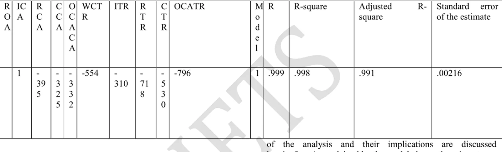
current assets has an impact on the profitability of the organization and one of the measures of profitability of an organization is Return on assets (ROA) and so an attempt has been made to check how inventory, debtors, cash and other current assets affect the performance of the firm. Correlation analysis is applied on data between the financial years 2009 to 2013. Return on Assets (ROA) is the dependant variable and its correlation is checked to a set a of independent variables like Inventory to Current assets(ICA), Receivables to Current Assets(RCA), cash to Current assets(CCA), other current assets to current assets(OCACA), Loans and advances to Current assets(LACA). Not only is the component of current assets important but the turnover of these current assets is also important. The turnover of current assets denotes theefficiency of the firm in managing them. As a rationale it is understood that efficiency means smooth conduct of operational activities, so a smooth conduct of operational activities should lead to higher profit for business. Thereby a correlation is also sought between Return on assets as an dependant variable and Working capital turnover ratio (WCTR), Inventory turnover ratio (ITR), Receivables Turnover Ratio (RTR), Cash turnover ratio (CTR), Other Current Assets turnover ratio (OCATR), loans and advances turnover ratio (LATR). Working capital management is basically about establishing a tradeoff between profitability and liquidity so a correlation is also sought between ROA and the liquidity ratios.
Table 5.1.a Current ratio (CR) and quick ratio (QR).
R O A IC A R C A C C A O C A C A WCT R
ITR R
T R
C T R
OCATR M
o d e l
R R-square Adjusted
R-square
Standard error of the estimate
1
-39 5 -3 2 5 -3 3 2
-554
-310 -71 8 -5 3 0
-796 1 .999 .998 .991 .00216
The results of correlation show that out of the thirteen ratios five ratios show negative correlation and eight ratios show positive correlation with Return on Assets (ROA). Of all the variables Other Current Assets Turnover Ratio (OCATR) and ROA have the highest correlation to the extent of 0.796 but negative in nature. The highest positive correlation ROA has is with Working Capital Turnover Ratio (WCTR). There is an almost insignificant correlation between Current Ratio and Quick Ratio and Return on Assets. Moreover, as it can be seen that of all the ratios turnover ratios have higher correlation with ROA which is true for a company like Mahindra and Mahindra who are basically a capital intensive company and turnover of assets plays a significant part in its operations. One can thereby conclude that ratios covering composition dimension and ratios indicating interrelationship between current assets and liabilities do not have a very high correlation with profitability but ratios covering the turnover dimension have high correlation with profitability.
5.2 Regression Analysis
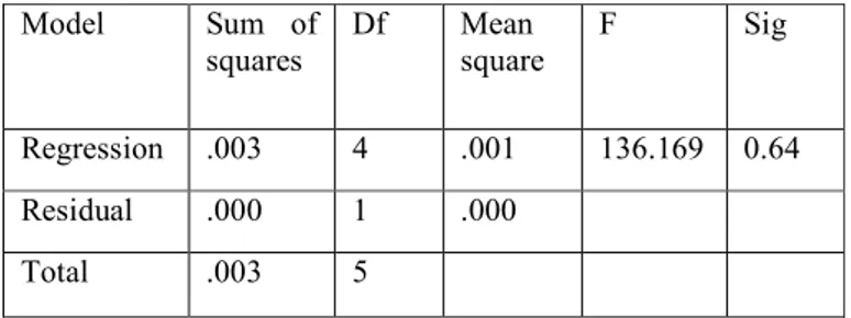
To further analyze the impact of significantly correlated independent variables on profitability of Mahindra and Mahindra, regression analysis was undertaken. The findings
of the analysis and their implications are discussed hereinafter. As explained by the model above, there is a strong correlation between the observed and the predicted value of Return on assets of Mahindra and Mahindra Ltd and the variation in value of ROA is considerably explained by this model. So, this model is optimistically fit for Mahindra and Mahindra Ltd. To further estimate the fitness of the model for the purpose of Mahindra and Mahindra, ANOVA values were calculated, which is exhibited below.
Model summary
Table 5.2 Regression Analysis
81
has a very negligible relationship. For the respondent company the following regression equation can be used to predict the value of dependant variables i.e. ROA.ROA = 0.154 + WCTR0.017+ITR0.01-RTR0.06
Model Sum of
squares
Df Mean
square
F Sig
Regression .003 4 .001 136.169 0.64
Residual .000 1 .000
Total .003 5
Table 5.2.a Multiple Regression Analysis Results
Note: SPSS version 6.0 is used to compute the results shown in the table from the original values of dependent and independent variables.
5.3 One-way Analysis of Variance Test (ANOVA)
It is useful for inter-unit comparisons. The following null and alternative hypotheses have been tested on the basis of ANOVA one-way analysis of variance test. H0: There is no any significant difference among the liquidity ratios of the selected Automobile companies in Indian automobile industry.
Results of the test of significance at 95% Confidence interval (that is, 0.05 level of significance) for liquidity indicated the following results.
VI-CONCLUSION
In this study, we analysis different type ratios examined for interpreting the results modern financial analysis have been carried out which minutely evaluates and examine relevant components for companies to smooth functioning ‘like’ Liquidity Analysis in which Current Ratio, Liquidity Ratio are tested, in Profitability Analysis in Relation to Sales G. P Ratio, N. P Ratio, O. P Ratio are tested and in Relation to Investment Return on Equity, Return on Assets, Return on Investment are tested, in Efficiency Analysis: Fixed Assets Turnover Ratio, Stock Turnover Ratio, Debtor Turnover Ratio are tested, in Leverage Analysis: Capital Gearing Ratio, Debt Equity Ratio, Interest Coverage Ratios are tested, in Market Value Analysis, Earnings Per Share, Price Earnings Ratio, Book Value Per Share are tested further, SD and CV, the Sum of Mean Values and Average score are calculated with example company.
REFERENCE
1. Arnold, G. (2008). Corporate Financial Management. 4th edit. Prentice Hall. Essex.
2. Baños-Caballero, S., García-Teruel, J.P. & Martínez-Solano, P. (2010). Working Capital Management in SMEs. Accounting and Finance, 50(2010). pp. 511 – 527.
3. Berry, A. & Jarvis, R. (2006). Accounting in a Business Context. Fourth Edition. London, UK: Thomson.
4. Besley, S. & Meyer, R. L. (1987). An Empirical Investigation of Factors Affecting the Cash Conversion Cycle. Annual Meeting of the Financial Management Association, Las Vegas, Nevada.
5. Bagavathi R.S.N. Pillai (2008)- Management Accounting, S.Chand & Company ltd, New Delhi.
6. Biais, B. & Gollier, C. (1997). Trade Credit and Credit Rationing. Review of Financial Studies, 10, pp. 903-937.
7. Carpenter, M. D. & Johnson, K. H. (1983). The Association Between Working Capital Policy and Operating Risk. Financial Review, 18(3), pp. 106-106.