VOLUME 36, ARTICLE 3, PAGES 73
−
110
PUBLISHED 5 JANUARY 2017
http://www.demographic-research.org/Volumes/Vol36/3/ DOI: 10.4054/DemRes.2017.36.3
Research Article
Parental separation and children’s education in
a comparative perspective: Does the burden
disappear when separation is more common?
Martin Kreidl
Martina Štípková
Barbora Hubatková
©2017 Martin Kreidl, Martina Štípková, Barbora Hubatková.
This open-access work is published under the terms of the Creative Commons Attribution NonCommercial License 2.0 Germany, which permits use, reproduction & distribution in any medium for non-commercial purposes, provided the original author(s) and source are given credit.
1 Introduction 74 2 Parental separation and children’s socioeconomic disadvantage 75 3 Variations in the effect of family disruption on educational
attainment
76 4 Comparative research on the effects of separation 78
5 Data and variables 79
6 Results 85
6.1 Binary logistic regression models 85 6.2 Random-intercept linear probability models 88
6.3 Sensitivity analyses 91
7 Conclusions and discussion 94
8 Acknowledgement 97
References 98
Parental separation and children’s education in
a comparative perspective:
Does the burden disappear when separation is more common?
Martin Kreidl1
Martina Štípková2
Barbora Hubatková3
Abstract
BACKGROUND
Parental breakup has, on average, a net negative effect on children’s education. However, it is unclear whether this negative effect changes when parental separation becomes more common.
OBJECTIVE
We studied the variations in the effect of parental separation on children’s chances of obtaining tertiary education across cohorts and countries with varying divorce rates.
METHOD
We applied country and cohort fixed-effect models as well as random-effect models to data from the first wave of the Generations and Gender Survey, complemented by selected macro-level indicators (divorce rate and educational expansion).
RESULTS
Country fixed-effect logistic regressions show that the negative effect of experiencing parental separation is stronger in more-recent birth cohorts. Random-intercept linear probability models confirm that the negative effect of parental breakup is significantly stronger when divorce is more common.
CONCLUSIONS
The results support the low-conflict family dissolution hypothesis, which explains the trend by a rising proportion of conflict breakups. A child from a dissolving
low-1
Office for Population Studies, Faculty of Social Studies, Masaryk University, Jostova 10, 60200 Brno, Czech Republic. E-Mail:[email protected].
2
Department of Sociology, University of West Bohemia, Univerzitni 8, 30614 Plzen, Czech Republic. E-Mail:[email protected].
3
conflict family is likely to be negatively affected by family dissolution, whereas a child from a high-conflict dissolving family experiences relief. As divorce becomes more common and more low-conflict couples separate, more children are negatively affected, and hence, the average effect of breakup is more negative.
CONTRIBUTION
We show a significant variation in the size of the effect of parental separation on children’s education; the effect becomes more negative when family dissolution is more common.
1. Introduction
Sociological and demographic investigations have repeatedly shown that parental breakup has negative effects on offspring. Children of separated parents, in comparison with children from two-parent families, have lower scores with respect to various dimensions of well-being (Amato and Keith 1991b), attain less education (Evans, Kelley, and Wanner 2001; Fischer 2007; Fronstin, Greenberg, and Robins 2001; Fučík 2016; Keith and Finlay 1988; Liu 2007), work in occupations of lower prestige, and have lower earnings (Amato and Keith 1991a; Fischer 2007), although this last finding may not be true for all genders (see Kiernan 1997).
While the negative impact of parental separation on children’s life chances is well-documented, less is known about long-term trends and cross-country differences in the strength of this effect. In this paper, we develop hypotheses on the change in the size of the negative effect of parental breakup over successive cohorts. We then generalize these arguments to differences across countries by linking variations in the association between parental breakup and children’s university graduation to the prevailing divorce rate. We test these hypotheses using both fixed-effect and random-effect multivariate models applied to data from 13 countries and four birth cohorts from cross-nationally harmonized surveys organized under the Generations and Gender Programme.
1995; Booth and Amato 2001; Hanson 1999; Jekielek 1998). As the incidence of family instability increases, the relative representation of low- and high-conflict couples among dissolving families changes: more and more low-conflict families split up, and the negative effects of breakup are encountered more frequently. At the population level, the negative consequences outweigh the positive, and the overall (average) negative effect becomes stronger as a result.
2. Parental separation and children’s socioeconomic disadvantage
Researchers have offered three main explanations as to why parental breakup negatively correlates with children’s educational attainment. One line of reasoning focuses on the stress associated with parental breakup, another emphasizes the economic and social deprivation associated with the changing household structure, and the last highlights selection into the breakup of parents with specific pre-existing qualities (Amato 1993, 2000).
Some authors emphasize that parental conflict before and during separation and the resulting stress are responsible for the negative outcomes in children (Amato 1993; Biblarz and Raftery 1999). Not only do offspring generally suffer from witnessing parental quarrels, but they are also directly involved and are forced to “choose sides.” The relationship between children and parents deteriorates as a result. Parental conflict can also serve as a bad behavioural and problem-solving example (Amato 1993). Children’s school outcomes are negatively impacted as a consequence.
The parental-adjustment perspective – an extension of the parental-conflict-and-stress argument – emphasizes the pivotal role of the psychological adjustment of the custodial parent after separation (Amato 1993). The effect on the child is dependent on the ability of the custodial parent to cope with the breakup and the resulting situation. The worse the parent copes, the stronger the detrimental effect on the children. This perspective is based on the view that stress interferes with parenting skills (Amato 1993). Since family dissolution is typically a stressful event, it is predicted “that decrements in the custodial parent’s…ability to function effectively in the parental role following marital dissolution can lower the well-being of children” (Amato 1993: 28).
and Li 2001, 2009). In extreme cases, an adolescent child may be forced to leave school and find a job to contribute to the family budget (Keith and Finlay 1988). Moreover, children in single-parent families lack support, efficient supervision, self-esteem, and relevant role models as a result of losing frequent contact with one of the parents; taken together, these factors also impact children’s life chances negatively (Amato and Booth 1991; Biblarz and Raftery 1999; Keith and Finlay 1988); Amato (1993) calls this argument “parental loss perspective.”
The selection argument proposes that individuals more prone to breakup also have poorer parenting skills (Amato 2000; Biblarz and Gottainer 2000; Biblarz and Raftery 1999; Holley, Yabiku, and Benin 2006). As summarized by Biblarz and Raftery (1999: 326), “People who divorce, for example, are less stable or less competent at family life. Children who experience their parents’ divorce do less well because their parents are less competent, not because of the divorce per se.…The divorce, like the negative child outcomes, may have been a consequence of some pre-existing family dysfunction.”
3. Variations in the effect of family disruption on educational
attainment
Parental separation has become a more common experience in most countries. We argue that this rising occurrence of family dissolution may have a changing impact on educational outcomes in children. Most theories predict a decrease in the negative effects of parental breakup on children across successive cohorts within countries. This expectation stems from three sources: increasingly tolerant attitudes and norms, liberalizing divorce legislation, and declining selection on poor parental skills. We call this expectation the easy-separation hypothesis. Yet one can also propose the opposite trend on the basis of declining levels of parental conflict associated with family dissolution. Accordingly, more recent cohorts of children of divorced couples contain a larger fraction of children among whom the negative consequences of family dissolution prevail, whereas only a declining proportion of children benefit from escaping a stressful family environment. We call this latter argument the low-conflict family dissolution hypothesis.
lesser degree (Becker 1993; Dronkers, Kalmijn, and Wagner 2006; Wolfinger 1999). Similarly, more-liberal divorce legislation makes separation less stressful and thus lessens the harm to both parents and children (Dronkers, Kalmijn, and Wagner 2006; Sigle-Rushton, Hobcraft, and Kiernan 2005). Finally, the negative effect of parental breakup may be diminishing because of declining self-selection (Kalmijn 2010): when family disruption becomes more common, couples splitting up should be less self-selected on poor parenting skills (Diekmann and Engelhardt 1999; Sigle-Rushton, Hobcraft, and Kiernan 2005).
The low-conflict family dissolution argument emphasizes the process perspective on family disruption (Luepnitz 1979; Morrison and Cherlin 1995; Sun 2001; Sun and Li 2001) and the parental-conflict explanation (Amato 2000; Amato, Loomis, and Booth 1995; Booth and Amato 2001; Hanson 1999); both lead to the prediction of increasing disadvantage when divorce is more widespread. Becker’s (1993) economic theory of marriage offers a similar prediction: as the specialization of men in market production and of women in household production declines, the gains from marriage become smaller (cf. Oppenheimer 1997 for a review of related literature). Therefore, even low-conflict and relatively well-functioning marriages often end in divorce (cf. Wolfinger 1999).
Amato and Hohmann-Marriott (2007) documented an increase in the incidence of dissolution in low-conflict marriages in the United States. Similarly, Gähler and Palmtag (2015) show declining levels of conflict – as reported retrospectively – by children from divorced families in Sweden. In earlier birth cohorts (born before 1919), three-quarters of children from dissolved marriages reported serious dissention in their childhood family. This proportion is approximately 60% in cohorts born around the middle of the 20th century and approximately 40% in cohorts born after 1970.
4. Comparative research on the effects of separation
Sociologists have been paying increasing attention to variations in the effects of family dissolution across subpopulations within countries since the 1990s (Amato 2000; Amato and Cheadle 2008; Bernardi and Radl 2014; Biblarz and Raftery 1993; Dronkers 1999; Kalmijn 2010; Kalmijn and Monden 2006; McLanahan and Sandefur 1994). Scholars, however, have focused much less on variations across societies. Notable exceptions studying the association between an individual’s divorce and well-being include Stack and Eshleman’s (1998) comparative study of 16 countries based on data from the 1980s, Diener and colleagues’ investigation of 42 countries in the 1990s (Diener et al. 2000), and Kalmijn’s recent study examining 38 countries from the European Value Study/World Value Study databases (Kalmijn 2010). While Stack and Eshleman’s (1998) examination indicated equality in the effects of marital status on well-being across countries, Diener and colleagues (2000) revealed a relatively weak negative association between the size of the divorce effect (i.e., the contrast between the married and the divorced) and the overall tolerance towards divorce in a country. Kalmijn’s (2010) analysis of respondents’ psychological well-being interacted several macro-level variables (e.g., divorce rate, church attendance, familialism, and approval of divorce) with an level indicator of divorce and found that the individual-level effect of divorce was somewhat weaker when divorce was more common.
Examinations of the stability of the effect of separation within countries are likewise rare, and even more so with children’s education as the dependent variable. Existing studies have achieved very ambiguous results. Evans, Kelley, and Wanner (2001) found that the detrimental effect of parental divorce on the odds of offspring graduating from secondary school increased over successive birth cohorts in Australia, while the effect of divorce on the likelihood of university graduation did not change. Ely and colleagues (1999) compared individuals born in 1946, 1958, and 1970 in Britain and found no change in the negative effect of divorce on education. Sigle-Rushton, Hobcraft, and Kiernan (2005) similarly identified no change in the divorce effect over cohorts in Britain. Gähler and Garriga (2013), who studied psychological maladjustment in children, did find a weakening effect of divorce between two Swedish surveys carried out in 1968 and 2000, but the result was not statistically significant. Bernardi and Radl (2014), on the other hand, identified a slight (and marginally statistically significant at the 0.1 level) interaction between parental breakup and divorce rate in a model of university graduation.
compared to their counterparts in two-biological-parent families (Garasky 1995; Raley, Frisco, and Wildsmith 2005), and remarriages are less stable than first marriages (Coleman, Ganong, and Fine 2000; Cherlin 1978, 1981; Furstenberg and Spanier 1984; Halliday 1980). Some authors argue that it is the experience of multiple family transitions, rather than the experience of family dissolution or any particular family type, that has the most pronounced impact on children (Aquilino 1996; Raley, Frisco, and Wildsmith 2005). Children of separated parents might be more socioeconomically disadvantaged in the context of high separation rates (and therefore in the context of more frequent repartnering and a higher number of transitions experienced in the household composition) than children of separated parents in contexts with less separation (and therefore less remarriage and more overall stability in the household composition).
Since the empirical evidence regarding variations in the size of the effect of family disruption on children’s education has so far been mixed (see above), our analysis aims to explore which of the hypotheses outlined above has more empirical support. Both of the hypotheses (the easy-separation hypothesis and the low-conflict family dissolution hypothesis) relate variations in the size of the breakup effect to changes in the prevalence of family disruption: is the negative effect of a breakup weaker (as predicted by the easy-separation hypothesis) when separation is more common, or is it stronger (as predicted by the low-conflict dissolution hypothesis)?
5. Data and variables
We use data from the first wave of surveys organized under the Generations and Gender Programme (United Nations 2005).4 This data set is unique because of its internationally comparative nature and the indicators contained in the questionnaire (it maps respondents’ family situations during childhood in a more detailed way, and it also contains cross-nationally harmonized measures of respondents’ and parents’ educational attainments). As of this writing, data from 19 countries is available in the GGP data archive. In principle, we wanted to use as many countries as possible, yet some countries could not be utilized; for instance, some could not be utilized because of variations in the definition of the sample or the unavailability of reasonably reliable measures of context-level variables. Therefore, we investigated 13 countries altogether: Australia, Belgium, Bulgaria, the Czech Republic, Estonia, France, Germany, Hungary, Italy, Lithuania, the Netherlands, Norway, and Romania. Interviews were conducted – depending on local circumstances – between 2001 and 2010.
4
The dependent variable in our analysis is a binary indicator of a respondent’s university graduation (coded 1 if the respondent ever completed university and 0 otherwise; university graduation implies category 5 or 6 on the ISCED scale included in the data set). We chose university graduation as our dependent variable for its international comparability in this data set. A dichotomous variable indicating whether a respondent’s parents broke up before their 18th birthday is our key explanatory variable. This measure is created using two questions from the questionnaire: the respondent’s experience of parental breakup5 and the respondent’s age when their parents broke up. The cutoff point at 18 years was chosen because students typically leave secondary education and enter tertiary education soon after their 18th birthday (cf. Fischer 2007).
In principle, family dissolution may affect children of any age (Liu 2007; Palosaari and Aro 1994). This general notion is mirrored in the literature, as there does not seem to be any widely used theory-based age limit beyond which parental divorce would be expected to have no effect. Age limits used in various analyses seem to be mostly chosen pragmatically, depending on the nature of the data (see, e.g., Chase-Lansdale, Cherlin, and Kiernan 1995; Fronstin, Greenberg, and Robins 2001; Furstenberg and Kiernan 2001; Kiernan 1997; Ross and Mirowsky 1999). When scholars face no data constraints, they use an array of different ages, usually without any detailed explanation. For example, the age limit used by Liu (2007) was 18 years; Garasky (1995), on the other hand, used 14 years, and some authors follow the incidence of parental divorce well into the respondents’ twenties (e.g., Aquilino 1994; Furstenberg and Kiernan 2001; Kiernan 1997). Overall, there is little consensus regarding what the most appropriate age limit is for such analyses, and so we chose the age of 18 years (as mentioned in the previous paragraph), but we also conducted all analyses with a different threshold – in our case, set at 15 years – to see if the results were sensitive to this particular decision (we report the sensitivity analyses in section 6.3).
We also used each respondent’s gender (coded 1 if male, 0 if female) and parental educational attainment as controls. Parental education was based on a slightly simplified ISCED scale and refers to the better-educated parent. We distinguished three substantive categories – up to lower secondary (ISCED 0‒2), upper secondary (ISCED
5 Breakup is not conceptually identical to divorce, but the GGS questionnaire does not let us distinguish
3‒4), and tertiary (ISCED 5‒6) – plus a separate category for respondents without a valid response.
Our analysis accounts for context-level characteristics in two ways. The first part of our analysis uses country and cohort fixed-effects, which is to say that both country and cohort are represented by a set of dummy indicators; 13 countries and 4 birth cohorts are differentiated (1940‒1949, 1950‒1959, 1960‒1969, and 1970+).6 The second part of our analysis utilizes random-intercept models, in which the macro-level contexts are defined by each unique combination of country and birth cohort. Since we have 13 countries and 4 birth cohorts, we examined 52 macro-level contexts. Our random-intercept models employ two continuous macro-level explanatory variables: crude divorce rate (CDR) and the percentage of individuals in each cohort attaining tertiary education. These variables were taken from external sources (the UN Demographic Yearbooks, Eurostat, and OECD).7 Divorce rate is our key theoretical concept (see above), whereas educational expansion is a control variable used to obtain unbiased estimates of the effects of the CDR (and its interactions) because educational expansion is correlated with divorce rates (both are typically higher in more-advanced societies) and also seems to have an impact on inequality of educational opportunity (see e.g., Shavit, Arum, and Gamoran 2007).
The proportion of respondents with tertiary education by country and cohort is shown in Figure 1. Clearly, enrolments grew in all countries. The share of people with tertiary education varies between 7% and 28% among individuals born in the 1940s, and then grows to 11%–34% in the cohorts born around 1960. The share of university graduates reached levels between 17% and 43% in the youngest birth cohorts in our analysis. The best-educated populations were in the Netherlands, Australia, Belgium, France, and Norway, while the least-educated populations were in Hungary, Romania, Italy, and the Czech Republic.
6
Although the data file contains individuals born before 1940, we set a birth-year limit to avoid distortions caused by unreliable historical macro-level data.
7
Figure 1: Proportion of people with tertiary education by birth cohort in selected countries
0
1
0
2
0
3
0
4
0
%
w
it
h
te
rt
ie
ry
e
d
u
c
a
ti
o
n
1940 1950 1960 1970 1980
Cohort
Australia Belgium Bulgaria
Czech Republic Estonia France
Germany Hungary Italy
Lithuania Netherlands Norway
Romania
Figure 2: Crude divorce rate (CDR) by year in selected countries
1
2
3
4
5
C
ru
d
e
d
iv
o
rc
e
ra
te
1940 1960 1980 2000
Year
Australia Belgium Bulgaria
Czech Republic Estonia France
Germany Hungary Italy
Lithuania Netherlands Norway
Romania
Macro-level contexts in multilevel models are defined by birth cohorts, but available divorce-rate data are period measures. We linked period measures to birth cohorts using the CDR at the time when cohort members’ parents typically broke up. We first computed the average age of the children at parental breakup (from the specific country/cohort combination) for those children who actually experienced parental breakup before their 18th birthday. We then added this number to the birth years of that particular cohort and thus obtained a reference period. The divorce-rate indicator is then the average CDR in the reference period. The average age at divorce for each country‒cohort combination is presented in the appendix.
The original data contained 130,244 cases (respondents). We limited the data set to individuals born after 1939 (see above). Furthermore, we only utilized respondents older than 26 years at the time of the interview to ensure that they had sufficient time to obtain tertiary education. These choices reduced the sample size to 94,502 cases (i.e., 73% of the original sample). After we deleted cases with missing data on the dependent variable (the respondent’s education), parental breakup, and the respondent’s gender, we obtained a final sample of 93,413 cases, which is to say that only 1% of eligible cases were lost because of missing responses (see Table 1). Some of the sensitivity analyses reported below may be based on a slightly different sample (this will be reemphasized in the relevant section).
Table 1: Sample characteristics by country. Selected countries from the Generations and Gender Survey (GGS), 2001‒2010
Country (1) Original sample size (2)
Within age limits (3)
Without missing values (4)
Per cent non-missing (5)a
Year of data collection (6)
Australia 7,125 4,826 4,770 99% 2005‒1006
Belgium 7,163 5,195 5,077 98% 2008‒2010
Bulgaria 12,858 8,751 8,672 99% 2004
Czech Republic 6,973 6,730 6,502 97% 2005
Estonia 7,855 5,371 5,346 100% 2004‒2005
France 10,079 7,051 6,961 99% 2005
Germany 10,017 6,900 6,792 98% 2005
Hungary 13,540 9,452 9,417 100% 2001‒2002
Italy 9,570 8,213 8,213 100% 2003
Lithuania 10,036 6,482 6,386 99% 2006
Netherlands 8,161 6,069 6,058 100% 2002‒2004
Norway 14,881 11,029 10,801 98% 2007‒2008
Romania 11,986 8,433 8,418 100% 2005
TOTAL 130,244 94,502 93,413 99% 2001‒2010
6. Results
6.1 Binary logistic regression models
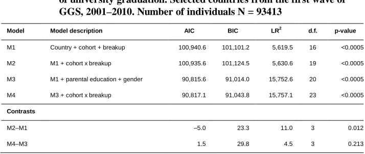
We begin with a series of binary logistic regressions predicting university graduation. The goodness-of-fit statistics of these models are presented in Table 2. As a first step, we want to see if the effect of parental breakup varies over cohorts within countries, both with and without statistical controls. Our first model contains only three predictors: parental breakup, country, and cohort (this is Model 1 in Table 2). Then we add the interaction between cohort and breakup to create Model 2. A statistical comparison of these two models tells us that – by criteria of classical inference – we should not omit the interaction from Model 2 (the likelihood-ratio test comparing these two models yields L2 = 11.0 with three degrees of freedom, which implies a p-value of 0.012). When judging by the two information criteria presented in Table 2 (AIC and BIC), we do not reach a clear conclusion – AIC suggests that we should favour the model with interactions, while BIC is in favour of the more parsimonious model. We carry out a similar test by comparing Model 3 and Model 4 (both contain controls for a respondent’s gender and parental education but are otherwise identical to Models 1 and 2, respectively). The comparison of Model 3 and Model 4 returns L2 = 4.5 (with 3 d.f.; p-value = 0.213), which indicates that the interaction between parental breakup and cohort is not statistically significant once the controls are introduced into the model. Also, AIC and BIC favour Model 3 over Model 4.
Table 2: Goodness-of-fit statistics of selected binary logistic regression models of university graduation. Selected countries from the first wave of GGS, 2001–2010. Number of individuals N = 93413
Model Model description AIC BIC LR2 d.f. p-value
M1 Country + cohort + breakup 100,940.6 101,101.2 5,619.5 16 <0.0005
M2 M1 + cohort x breakup 100,935.6 101,124.5 5,630.6 19 <0.0005
M3 M1 + parental education + gender 90,815.6 91,014.0 15,752.6 20 <0.0005
M4 M3 + cohort x breakup 90,817.1 91,043.8 15,757.1 23 <0.0005
Contrasts
M2–M1 ‒5.0 23.3 11.0 3 0.012
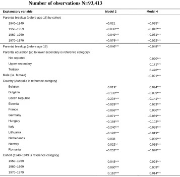
Average marginal effects (rather than logistic coefficients ‒ see Mood 2010) are used to evaluate Model 2 (see Table 3). We see that the effect of parental breakup is weak (breakup seems to reduce the probability of university graduation by 2 percentage points) and statistically insignificant in the 1940‒1949 birth cohort. The effect of breakup becomes more negative in each subsequent birth cohort. For instance, parental separation reduces the probability of university completion by 3.6%, 4.9%, and 7.9% in the 1950‒1959, 1960‒1969, and 1970‒1979 birth cohorts, respectively. These values are statistically significantly different from 0 (at the 0.01 level ‒ see Table 3). Thus, overall, the estimated negative effect of parental breakup grew by 5.8 percentage points, and the difference between the breakup effect in the first and the last cohort is statistically significantly different from 0 (at the 0.01 level).
Table 3 also presents average marginal effects based on Model 4. We have seen that the interaction between parental breakup and cohort fails to reach standard levels of statistical significance in Model 4. Yet when we look at the development of the average marginal effects of breakup across cohorts, we see the pattern of an increasingly negative effect. For instance, Model 4 indicates that family dissolution lowers the probability of university graduation by 3.5 percentage points in the oldest cohort. This disadvantage grows to 4.2%, 5.1%, and 6.2% in the 1950‒1959, 1960‒1969, and 1970‒1979 birth cohorts, respectively. All of these effects are statistically significantly different from 0 (at least at the 0.05 level, see Table 3). The effect increases by 2.7 percentage points over cohorts in Model 4, and the growth (i.e., the difference between the eldest and the youngest cohort) is statistically significantly different from 0 at the 0.1 level.
The change in the net effect of breakup in Model 4 achieves a lower significance level than in Model 2 because of the confounding effect of parental education: better-educated parents were more likely to break up in the older cohorts, and the negative net effect of family dissolution was (partially) offset by the positive effect of parental education. This confounding effect became less salient (or even disappeared) in more-recent cohorts with the reversal of the education gradient of divorce (Härkönen and Dronkers 2006; Matysiak, Styrc, and Vignoli 2014).
obtaining a university degree increases by 47 percentage points among children of tertiary-educated parents in comparison with children whose parents only attained a lower-secondary (or lower) level of education (see Table 3).
Table 3: Average marginal effects from binary logistic regression models of university graduation. Selected countries from the GGS, 2001‒2010. Number of observations N=93,413
Explanatory variable Model 2 Model 4
Parental breakup (before age 18) by cohort
1940‒1949 ‒0.021 ‒0.035**
1950‒1959 ‒0.036*** ‒0.042***
1960‒1969 ‒0.049*** ‒0.051***
1970‒1979 ‒0.079*** ‒0.062***
Parental breakup (before age 18) ‒0.046*** ‒0.048***
Parental education (up to lower secondary is reference category)
Not reported 0.020***
Upper secondary 0.171***
Tertiary 0.470***
Male (vs. female) ‒0.021***
Country (Australia is reference category)
Belgium 0.019* 0.094***
Bulgaria ‒0.133*** ‒0.039***
Czech Republic ‒0.204*** ‒0.141***
Estonia ‒0.029*** 0.033***
France ‒0.066*** 0.050***
Germany ‒0.071*** ‒0.069***
Hungary ‒0.184*** ‒0.103***
Italy ‒0.240*** ‒0.099***
Lithuania ‒0.126*** ‒0.019**
Netherlands 0.008 0.096***
Norway 0.022** 0.039***
Romania ‒0.252*** ‒0.098***
Cohort (1940‒1949 is reference category)
1950‒1959 0.043*** 0.024***
1960‒1969 0.060*** 0.009**
1970‒1979 0.110*** 0.014***
6.2 Random-intercept linear probability models
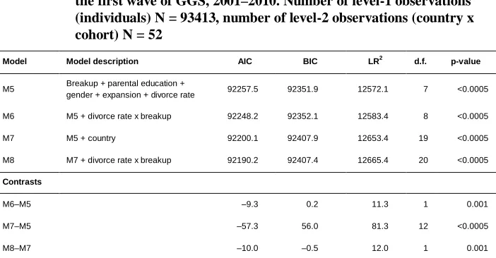
Now we proceed to multilevel random-intercept linear probability models (LPMs). We chose multilevel LPMs rather than multilevel logistic regression models because the statistical toolkit to obtain robust estimates of multilevel logistic regression models (and to translate them to average marginal effects) is not sufficiently developed; moreover, the interpretation of interaction effects in logistic regression and the comparison of effects across logistic regression models is problematic (Mood 2010). We use two different specifications of the multilevel model. We start with two continuous variables – the CDR and the share of individuals with tertiary education (these macro-variables are utilized along with micro-level covariates such as gender, parental education, and parental breakup). The second specification also adds country fixed-effects into the model. We use this latter specification to ensure that our results are not biased by some omitted country-level variables such as education- or family-related policies.
Table 4: Goodness-of-fit statistics of selected random-intercept linear
probability models of university graduation. Selected countries from the first wave of GGS, 2001–2010. Number of level-1 observations (individuals) N = 93413, number of level-2 observations (country x cohort) N = 52
Model Model description AIC BIC LR2 d.f. p-value
M5 Breakup + parental education +
gender + expansion + divorce rate 92257.5 92351.9 12572.1 7 <0.0005
M6 M5 + divorce rate x breakup 92248.2 92352.1 12583.4 8 <0.0005
M7 M5 + country 92200.1 92407.9 12653.4 19 <0.0005
M8 M7 + divorce rate x breakup 92190.2 92407.4 12665.4 20 <0.0005
Contrasts
M6–M5 ‒9.3 0.2 11.3 1 0.001
M7–M5 ‒57.3 56.0 81.3 12 <0.0005
M8–M7 ‒10.0 ‒0.5 12.0 1 0.001
without this interaction. AIC and BIC values are based on the deviance statistic and are computed using the formulas proposed by Hox (2010: 50‒51); the number of individual respondents is used as the number of observations in the calculation of BIC (see STATA Corp. 2011: 159‒163).8 Table 4 presents the goodness-of-fit statistics of all multilevel models.
Model 5 employs all explanatory variables additively, while Model 6 also adds the cross-level interaction between breakup and divorce rate. By the criteria of classical statistical inference, we should prefer Model 6 to Model 5, which is to say that we should not omit the interaction from the model (the comparison of the two models leads to L2 = 11.3 with one degree of freedom, which implies p = 0.001). Again, AIC and BIC tend to contradict each other – AIC favours keeping the interaction, whereas BIC indicates no difference in model fit between the models, in which case the more parsimonious Model 5 should be preferred. We are inclined to keep the interaction in the model and inspect its substantive significance.
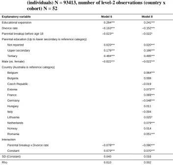
The estimated effects of Model 6 are presented in Table 5. We see from the main effect of parental breakup that parental separation has a slight negative effect on the probability of university graduation when the CDR is 0, which is to say, when the divorce rate is at its minimum observed in the data: the probability of university graduation for a child whose parents broke up is lower by 2.3 percentage points (the effect is significantly different from 0 at the 0.05 level). The interaction between parental breakup and divorce rate tells us that the effect of breakup becomes more negative with higher divorce rates (the interaction is statistically significantly different from 0 at the 0.001 level ‒ see Table 5). When the divorce rate reaches its maximum in our data set, the effect of parental breakup on the probability of university graduation is ‒10.1 (= ‒0.023‒0.078 ‒ see Model 6 in Table 5), which is to say, more than four times higher than it was at the minimal divorce rate.
Models 7 and 8 also contain country fixed-effects in addition to all of the effects already present in Models 5 and 6; thus, Models 7 and 8 control for the confounding effects of all other country-level factors such as policies, values, and norms and therefore provide evidence that is less susceptible to omitted-variable bias. Yet comparing Models 7 and 8 leads to the same conclusion that we reached earlier: we should keep the cross-level interaction between parental breakup and CDR in the model (by the criteria of classical inference, the test of the hypothesis that the interaction is in fact zero leads to L2 = 12.0 with 1 d. f., p = 0.001; also, AIC is in favour of keeping the interaction, whereas BIC is not ‒ see Table 4). Thus, parental breakup seems to interact
8
with the CDR even within countries. This feature of the last model is worth emphasizing: Model 8 (with country fixed-effects) minimizes the risk of bias due to omitted macro-variables.
Table 5: Estimated coefficients of selected random-intercept linear probability models of university graduation. Selected countries from the first wave of GGS, 2001–2010. Number of level-1 observations
(individuals) N = 93413, number of level-2 observations (country x cohort) N = 52
Explanatory variable Model 6 Model 8
Educational expansion 0.284*** 0.241***
Divorce rate ‒0.163*** ‒0.152***
Parental breakup before age 18 ‒0.023** ‒0.022*
Parental education (Up to lower secondary is reference category)
Not reported 0.020*** 0.020***
Upper secondary 0.176*** 0.186***
Tertiary 0.484*** 0.485***
Male (vs. female) ‒0.022*** ‒0.022***
Country (Australia is reference category)
Belgium 0.064***
Bulgaria 0.008
Czech Republic ‒0.019
Estonia 0.073***
France 0.069***
Germany ‒0.048***
Hungary 0.011
Italy ‒0.004
Lithuania 0.025*
Netherlands 0.079***
Norway 0.014
Romania 0.051***
Interaction
Parental breakup x Divorce rate ‒0.078*** ‒0.080***
Constant 0.079*** 0.070***
SD (Constant) 0.040 0.016
Rho 0.010 0.002
Inspecting the estimated parameters of Model 8 (see Table 5), we again see that the negative net effect of parental breakup becomes more negative when divorce rates are higher. For instance, the negative effect of parental breakup on the probability of university completion is ‒0.022 when the divorce rate is at its minimum level (this effect is statistically significantly different from 0 at the 0.1 level). The negative effect of breakup grows to ‒0.102 (= ‒0.022‒0.080 ‒ see Table 5) when the divorce rate reaches its maximum (i.e., the growth is more than fourfold). Other effects in Model 8 bring no surprises: males, on average, have lower chances of obtaining a university diploma; parental education has a strong positive effect on a respondent’s education; educational expansion seems to improve the chances of graduating from university; and divorce rate, net of everything else in the model, has a negative effect on educational attainment.
6.3 Sensitivity analyses
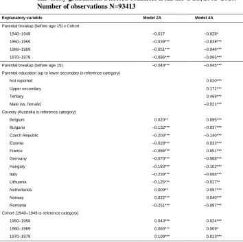
Redefining the main explanatory variable (parental breakup before the age of 18 years) and using a different cutoff age has no apparent effect on the results. When we move the decisive cutoff point to 15 years and re-estimate all models, we still see the same patterns of interactions. For instance, in Model 2A (a modified version of Model 2), the average marginal effect of breakup goes up from ‒0.017 in the oldest cohort to ‒0.086 in the most recent cohort (see Table 6, Model 2A), i.e., by 6.9 percentage points, which is a slightly stronger increase than in Model 2 (where the effect grew by 5.8 percentage points; see Table 3 above). The contrast between the breakup effect in the oldest and youngest cohorts is statistically significantly different from 0 at the 0.01 level.
Table 6: Average marginal effects from binary logistic regression models of university graduation. Selected countries from the GGS, 2001‒2010. Number of observations N=93413
Explanatory variable Model 2A Model 4A
Parental breakup (before age 15) x Cohort
1940‒1949 ‒0.017 ‒0.028*
1950‒1959 ‒0.039*** ‒0.038***
1960‒1969 ‒0.051*** ‒0.046***
1970‒1979 ‒0.086*** ‒0.065***
Parental breakup (before age 15) ‒0.048*** ‒0.045***
Parental education (up to lower secondary is reference category)
Not reported 0.020***
Upper secondary 0.171***
Tertiary 0.469***
Male (vs. female) ‒0.021***
Country (Australia is reference category)
Belgium 0.020** 0.095***
Bulgaria ‒0.132*** ‒0.037***
Czech Republic ‒0.203*** ‒0.140***
Estonia ‒0.028*** 0.033***
France ‒0.066*** 0.051***
Germany ‒0.070*** ‒0.068***
Hungary ‒0.183*** ‒0.102***
Italy ‒0.239*** ‒0.098***
Lithuania ‒0.125*** ‒0.017**
Netherlands 0.009** 0.097***
Norway 0.022*** 0.040***
Romania ‒0.251*** ‒0.097***
Cohort (1940‒1949 is reference category)
1950‒1959 0.043*** 0.024***
1960‒1969 0.060*** 0.009*
1970‒1979 0.109*** 0.013***
*** p<0.01, ** p<0.05, * p<0.1
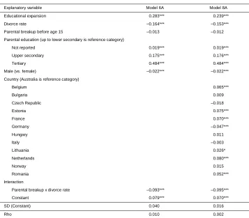
(Table 7). The interaction between breakup and the CDR is statistically significant at the 0.01 level in both models.
Table 7: Estimated coefficients of selected random-intercept linear probability models of university graduation. Selected countries from the first wave of GGS, 2001‒2010. Number of level-1 observations
(individuals) N = 93413, number of level-2 observations (country x cohort) N = 52
Explanatory variable Model 6A Model 8A
Educational expansion 0.283*** 0.239***
Divorce rate ‒0.164*** ‒0.153***
Parental breakup before age 15 ‒0.013 ‒0.012
Parental education (up to lower secondary is reference category)
Not reported 0.019*** 0.019***
Upper secondary 0.175*** 0.176***
Tertiary 0.484*** 0.484***
Male (vs. female) ‒0.022*** ‒0.022***
Country (Australia is reference category)
Belgium 0.065***
Bulgaria 0.009
Czech Republic ‒0.018
Estonia 0.075***
France 0.070***
Germany ‒0.047***
Hungary 0.011
Italy ‒0.003
Lithuania 0.026*
Netherlands 0.080***
Norway 0.015
Romania 0.052***
Interaction
Parental breakup x divorce rate ‒0.093*** ‒0.095***
Constant 0.079*** 0.070***
SD (Constant) 0.040 0.016
Rho 0.010 0.002
Furthermore, we wanted to see if any country in our sample may have had a particularly strong influence on the findings. To establish this, we tested whether the omission of any single country from the sample would alter the results and found that our conclusions are very robust. The results for these alternative samples for Model 4 (binary logit with all individual-level controls) and for Model 6 (multilevel LPM) are as follows: While the negative average marginal effect of parental separation grew from ‒0.035 to ‒0.062 in Model 4 (that is, by 2.7 percentage points, see Table 3), this increase ranged from 1.3 percentage points when Estonia was omitted (the second-lowest value was 1.9, when Australia was not in the sample) to 3.6 percentage points when Germany was left out of the sample (the second-largest value of 3.4 percentage points was achieved when either Hungary or the Netherlands were omitted from the sample).
Re-estimations of Model 6 confirm that the cross-level interaction between breakup and the CDR persists even when the sample of countries is redefined. While the interaction was ‒0.078 in Model 6, it ranged between ‒0.061 (when Australia was not in the sample) and ‒0.092 (when Hungarian data was not used). The interaction was statistically significant at the 0.05 level (when the Australian sample was not included in the analysis), and was significant at the 0.01 level in all other re-estimations. Thus, we are confident that the results are not driven by one particular country.
7. Conclusions and discussion
almost 10 percentage points when the CDR reaches its maximum (i.e., it is five times stronger).
One may suspect that our models – with only two macro-level variables (CDR and educational expansion) – are too parsimonious to capture all relevant variation across contexts and that the estimated macro-level effects (and their interactions) are consequently prone to omitted-variable bias. It may be especially tempting to point to prevailing values and norms as well as the level of welfare and intergenerational transfers as potential sources of model misspecification. We have, therefore, run all random-intercept models also with country fixed-effects to minimize the risk of bias, and we showed that the interaction between parental separation and the CDR persists even with this alternative specification. When we add country fixed-effects, we effectively statistically control for the confounding effects of all measured and unmeasured country-level characteristics, at least to the extent that these are reasonably robust over time and have an additive effect on the outcome. Working with country fixed-effects is equivalent to carrying out a within-country analysis of the trend, and it serves as a robust check. Thus, CDR interacts with parental separation both within and across countries. One can, of course, argue that there are other context-level variables (such as family policies or female employment rates) that change relatively rapidly and/or may interact with the effect of parental separation. Yet it seems that the inclusion of such additional macro-level variables may not be easy to achieve, since the sample size is modest and some of the effects were already only borderline statistically significant. Nevertheless, such an analysis would nicely complement ours and it is, no doubt, a worthwhile research enterprise that should be carried out as soon as the data permits.
The results seem to support the low-conflict family dissolution hypothesis. This hypothesis stems from observations that as family dissolution becomes more common, even couples experiencing less conflict separate (Amato and Hohmann-Marriott 2007; Gähler and Palmtag 2015). When a low-conflict family dissolves, the child is negatively affected. With increasing familial instability, low-conflict families predominate in the population of separating parents, and thus, the negative consequences (among a growing share of children) outweigh the positive ones (i.e., ones that may result when a high-conflict family breaks up), at least on average.
current Generations and Gender Survery (GGS) database does not – in our opinion – permit a more complex test.
Our main finding holds vis-à-vis partial model respecifications and appears to be robust. For instance, we used both standard binary logistic regression and multilevel linear probability models (with and without several level-1 controls) and identified consistent substantive findings. We used random-intercept models with and without country fixed-effects to confirm that the key interaction between parental separation and divorce rate holds both within and across countries. Moreover, modifying the operational definition of the main explanatory variable (parental separation) and taking all breakups before the age of 15 years (instead of the age of 18 years, as we did in the main part of the analysis) leaves the results virtually unchanged. Similarly, a redefinition of the set of countries has little effect on our findings, and the results do not seem to be driven by outliers.
Our results seem to be in contrast with those of Kalmijn (2010), who studied the effect of one’s own divorce on one’s own well-being (i.e., the effects of divorce among adults) and showed that the negative effect diminishes when divorce becomes more common. The reasons for such inconsistency might be two-fold. First, we studied the consequences of parental separation on children, while Kalmijn investigated the divorcees themselves. It is possible that divorce affects adults (who are more directly involved in making decisions about divorce) differently than children (who have little power to influence their parents’ separation). For instance, at least some adults may choose divorce correctly anticipating that their well-being will improve thereafter, and therefore, the average negative effect of divorce may be driven towards zero. This may occur more frequently in countries with a higher prevalence of divorce. If the share of these adults increases, the average effect of divorce would diminish. Yet the same logic does not apply to children. Second, the outcome variables differ. We focused on educational attainment (university graduation), while Kalmijn studied the self-reported level of well-being. While any disruption of an educational career may have a lasting effect, well-being may improve over time, for instance after remarriage (Shapiro 1996; Weingarten 1980, 1985). Since divorce and remarriage rates tend to be correlated, people have enjoyed the positive effects of remarriage more often in recent decades, and thus the effect of divorce is mitigated by remarriage. However, parental remarriage may not have the same positive consequence for children’s schooling, since stepparents might be less willing to invest in the education of their stepchildren, preferring to support their biological children (Case, Lin, and McLanahan 2001; Pong 1997; Stewart 2010; Tillman 2007).
that children from dysfunctional homes experience in their lives. Furthermore, this finding suggests that stratification scholars should pay more attention to the effects of growing variability in the family forms experienced by children. This variability includes, but is not limited to, children of divorced parents, cohabiting parents, single parents, and stepparents, all of whom are increasingly present in many developed societies.
8. Acknowledgement
References
Amato, P.R. (1993). Children’s adjustment to divorce: Theories, hypotheses, and empirical support.Journal of Marriage and Family 55(1): 23–38. doi:10.2307/ 352954.
Amato, P.R. (2000). Consequences of divorce for adults and children. Journal of
Marriage and Family 62(4): 1269–1287. doi:10.1111/j.1741-3737.2000.012
69.x.
Amato, P.R. and Booth, A. (1991). Consequences of parental divorce and marital unhappiness for adult well-being. Social Forces 69(3): 895–914. doi:10.1093/ sf/69.3.895.
Amato, P.R. and Cheadle, J. (2008). Parental divorce, marital conflict and children’s behavior problems: A comparison of adopted and biological children. Social
Forces86(3): 1139–1161.doi:10.1353/sof.0.0025.
Amato, P.R. and Hohmann-Marriott, B. (2007). Comparison of high- and low-distress marriages that end in divorce. Journal of Marriage and Family 69(3): 621–638.
doi:10.1111/j.1741-3737.2007.00396.x.
Amato, P.R. and Keith, B. (1991a). Parental divorce and adult well-being: A meta-analysis.Journal of Marriage and Family 53(1): 43–58.doi:10.2307/353132.
Amato, P.R. and Keith, B. (1991b). Parental divorce and the well-being of children: A meta-analysis. Psychological Bulletin 110(1): 26–46. doi:10.1037/0033-2909. 110.1.26.
Amato, P.R., Loomis, L.S., and Booth, A. (1995). Parental divorce, marital conflict, and offspring well-being during early adulthood. Social Forces 73(3): 895–915.
doi:10.1093/sf/73.3.895.
Andersson, G. (2002). Children’s experience of family disruption and family formation: Evidence from 16 countries. Demographic Research 7(7): 343–364.
doi:10.4054/DemRes.2002.7.7.
Aquilino, W.S. (1996). The lifecourse of children born to unmarried mothers: Childhood living arrangements and young adult outcomes. Journal of Marriage
and the Family 58(2): 293–310.doi:10.2307/353496.
Bernardi, F. and Radl, J. (2014). The long-term consequences of parental divorce for children’s educational attainment. Demographic Research 30(61): 1653‒1680.
doi:10.4054/DemRes.2014.30.61.
Biblarz, T.J. and Raftery, A.E. (1993). The effects of family disruption on social mobility.American Sociological Review 58(1): 97‒109.doi:10.2307/2096220.
Biblarz, T.J. and Raftery, A.E. (1999). Family structure, educational attainment, and socioeconomic success: Rethinking the ‘pathology of matriarchy.’ American
Journal of Sociology 105(2): 321–365.doi:10.1086/210314.
Biblarz, T.J. and Gottainer, G. (2000). Family structure and children’s success: A comparison of widowed and divorced single-mother families. Journal of
Marriage and Family 62(2): 533–548.doi:10.1111/j.1741-3737.2000.00533.x.
Booth, A. and Amato, P.R. (2001). Parental predivorce relations and offspring postdivorce well-being. Journal of Marriage and Family 63(1): 197–212.
doi:10.1111/j.1741-3737.2001.00197.x.
Brown, S.L. (2004). Family structure and child well-being: The significance of parental cohabitation. Journal of Marriage and Family 66(2): 351–367. doi:10.1111/ j.1741-3737.2004.00025.x.
Buchmann, C. and DiPrete, T.A. (2006). Growing female advantage in college completion: The role of family background and academic achievement.
American Sociological Review 71(4): 515–541. doi:10.1177/00031224060710
0401.
Bulanda, R.E. and Manning, W.D. (2008). Parental cohabitation experience and adolescent behavioral outcomes.Population Research and Policy Review 27(5): 593–618.doi:10.1007/s11113-008-9083-8.
Case, A., Lin, I-F., and McLanahan, S. (2001). Educational attainment of siblings in stepfamilies. Evolution and Human Behavior 22(4): 269–289. doi:10.1016/S10 90-5138(01)00069-1.
Chase-Lansdale, P.L., Cherlin, A.J., and Kiernan, K.E. (1995). The long-term effects of parental divorce on mental health of young adults: A developmental perspective.
Child Development 66(6): 1614–1634.doi:10.2307/1131900.
Cherlin, A. (1978). Remarriage as an incomplete institution. American Journal of
Sociology84(3): 634–650.
Coleman, M., Ganong, L., and Fine, M. (2000). Reinvestigating remarriage: Another decade of progress. Journal of Marriage and Family 62(4): 1288–1307.
doi:10.1111/j.1741-3737.2000.01288.x.
Diekmann, A. and Engelhardt, H. (1999). The social inheritance of divorce: Effects of parent’s family type in postwar Germany.American Sociological Review 64(6): 783–793.doi:10.2307/2657402.
Diener, E., Gohm, C.L., Suh, E., and Oishi, S. (2000). Similarity of the relations between marital status and subjective well-being across cultures. Journal of
Cross-Cultural Comparison 31(4): 419–436. doi:10.1177/002202210003100
4001.
Dronkers, J. (1999). The effects of parental conflicts and divorce on the well-being of pupils in Dutch secondary education.European Sociological Review 15(2): 195– 212.doi:10.1093/oxfordjournals.esr.a018260.
Dronkers, J., Kalmijn, M., and Wagner, M. (2006). Causes and consequences of divorce: Cross-national and cohort differences, an introduction to this special issue.European Sociological Review 22(5): 479–481.doi:10.1093/esr/jcl015.
Ely, M., Richards, M.P.M., Wadsworth, M.E.J., and Elliott, B.J. (1999). Secular changes in the association of parental divorce and children’s educational attainment: Evidence from three British birth cohorts. Journal of Social Policy
28(3): 437–455.doi:10.1017/S0047279499005693.
Evans, M.D.R., Kelley, J., and Wanner, R.A. (2001). Educational attainment of the children of divorce: Australia, 1940‒90.Journal of Sociology 37(3): 275–297.
doi:10.1177/144078301128756346.
Fischer, T. (2007). Parental divorce and children’s socio-economic success: Conditional effects of parental resources prior to divorce, and gender of the child.Sociology
41(3): 475–495.doi:10.1177/0038038507076618.
Fronstin, P., Greenberg, D.H., and Robins, P.K. (2001). Parental disruption and the labour market performance of children when they reach adulthood. Journal of
Population Economics 14(1): 137–172.doi:10.1007/s001480050163.
Furstenberg, F.F. and Kiernan, K. (2001). Delayed parental divorce: How much do children benefit?Journal of Marriage and Family 63(2): 446–457.doi:10.1111/ j.1741-3737.2001.00446.x.
Furstenberg, F.F. and Spanier, G.B. (1984). The risk of dissolution in remarriage: An examination of Cherlin’s hypothesis of incomplete institutionalization. Family
Relations33(3): 433–441.doi:10.2307/584714.
Gähler, M. and Garriga, A. (2013). Has the association between parental divorce and young adults’ psychological problems changed over time? Evidence from Sweden, 1968‒2000.Journal of Family Issues 34(6): 784–808.doi:10.1177/01 92513X12447177.
Gähler, M. and Palmtag, E.L. (2015). Parental divorce, psychological well-being and educational attainment: Changed experience, unchanged effect among Swedes born 1892–1991. Social Indicators Research123(2): 601‒623. doi:10.1007/s11 205-014-0768-6.
Garasky, S. (1995). The effect of family structure on educational attainment: Do the effects vary by the age of the child? American Journal of Economics and
Sociology 54(1): 89–105.doi:10.1111/j.1536-7150.1995.tb02633.x.
González, L. and Viitanen, T.K. (2006). The effect of divorce laws on divorce rates in Europe (IZA discussion paper no. 2023). Bonn: Institute for the Study of Labor. Retrieved December 10, 2012, fromhttp://ftp.iza.org/dp2023.pdf.
Goode, W.J. (1993).World changes in divorce patterns. New Haven: Yale University Press.
Halliday, T.C. (1980). Remarriage: The more complete institution?American Journal
of Sociology86(3): 630–635.doi:10.1086/227285.
Hanson, T.L. (1999). Does parental conflict explain why divorce is negatively associated with child welfare? Social Forces 77(4): 1283–1316. doi:10.1093/ sf/77.4.1283.
Härkönen, J. and Dronkers, J. (2006). Stability and change in the educational gradient of divorce: A comparison of seventeen countries.European Sociological Review
22(5): 501–517.doi:10.1093/esr/jcl011.
Hox, J. (2010).Multilevel analysis: Techniques and applications(2nd ed.). New York: Routledge.
Jekielek, S.M. (1998). Parental conflict, marital disruption and children’s emotional well-being.Social Forces76(3): 905‒936.doi:10.1093/sf/76.3.905.
Kalmijn, M. (2010). Country differences in the effects of divorce on well-being: The role of norms, support, and selectivity. European Sociological Review 26(4): 475–490.doi:10.1093/esr/jcp035.
Kalmijn, M. and Monden, C.W.S. (2006). Are the negative effects of divorce on well-being dependent on marital quality? Journal of Marriage and Family 68(5): 1197–1213.doi:10.1111/j.1741-3737.2006.00323.x.
Kalmijn, M. and Uunk, W. (2007). Regional value differences in Europe and the social consequences of divorce: A test of the stigmatization hypothesis.Social Science
Research 36(2): 447–468.doi:10.1016/j.ssresearch.2006.06.001.
Keith, V.M. and Finlay, B. (1988). The impact of divorce on children’s educational attainment, marital timing, and likelihood of divorce. Journal of Marriage and
Family 50(3): 797–809.doi:10.2307/352648.
Kennedy, S. and Bumpass, L. (2008). Cohabitation and children’s living arrangements: New estimates from the United States. Demographic Research 19(47): 1663– 1692.doi:10.4054/DemRes.2008.19.47.
Kiernan, K. (1997). The legacy of parental divorce: Social, economic and demographic experiences in adulthood (CASE paper 1). London: London School of Economics, Centre for Analysis of Social Exclusion.
http://eprints.lse.ac.uk/6535/1/The_Legacy_of_Parental_Divorce_Social,_econo mic_and_demographic_experiences_in_adulthood.pdf.
Liu, S. H. (2007). The effect of parental divorce and its timing on child educational attainment: A dynamic approach. http://moya.bus.miami.edu/~sliu/Research_ files/divorcetiming.pdf.
Luepnitz, D.A. (1979). Which aspects of divorce affect children? The Family
Coordinator 28(1): 79–85.doi:10.2307/583272.
Manning, W.D. and Lamb, K. (2003). Adolescent well-being in cohabiting, married, and single-parent families. Journal of Marriage and Family 65(4): 876–893.
Manning, W.D., Smock, P.J., and Majumdar, D. (2004). The relative stability of cohabiting and marital unions for children. Population Research and Policy
Review 23(1): 135–159.doi:10.1023/B:POPU.0000019916.29156.a7.
Matysiak, A., Styrc, M., and Vignoli, D. (2014). The educational gradient in marital disruption: A meta-analysis of European research findings. Population Studies
68(2): 197–215.doi:10.1080/00324728.2013.856459.
McLanahan, S. and Sandefur, G. (1994).Growing up with a single parent: What hurts,
what helps?Cambridge: Harvard University Press.
Mood, C. (2010). Logistic regression: Why we cannot do what we think we can do and what we can do about it.European Sociological Review 26(1): 67‒82.
doi:10.1093/esr/jcp006.
Morrison, D.R. and Cherlin, A.J. (1995). The divorce process and young children’s well-being: A prospective analysis.Journal of Marriage and Family 57(3): 800– 812.doi:10.2307/353933.
Nock, S.L. (1995). A comparison of marriages and cohabiting relationships.Journal of
Family Issues 16(1): 53–76.doi:10.1177/019251395016001004.
Oppenheimer, V.K. (1997). Women’s employment and the gain to marriage: The specialization and trading model. Annual Review of Sociology 23: 431–453.
doi:10.1146/annurev.soc.23.1.431.
Palosaari, U. and Aro, H. (1994). Effect and timing of parental divorce on the vulnerability to depression in young adulthood.Adolescence 29(115): 681–690.
Pong, S.-L. (1997). Family structure, school context, and eighth-grade math and reading achievement. Journal of Marriage and Family 59(3): 734–746. doi:10.2307/ 353957.
Raley, R.K., Frisco, M.L., and Wildsmith, E. (2005). Maternal cohabitation and educational success. Sociology of Education 78(2): 144–164. doi:10.1177/003 804070507800203.
Ross, C.E. and Mirowsky, J. (1999). Parental divorce, life-course disruption, and adult depression. Journal of Marriage and Family 61(4): 1034–1045. doi:10.2307/ 354022.
Shapiro, A.D. (1996). Explaining psychological distress in a sample of remarried and divorced persons: The influence of economic distress. Journal of Family Issues
Shavit, Y., Arum, R., and Gamoran, A. (eds.) (2007).Stratification in higher education. Stanford: Stanford University Press.
Sigle-Rushton, W., Hobcraft, J., and Kiernan, K. (2005). Parental divorce and subsequent disadvantage: A cross-cohort comparison.Demography 42(3): 427– 446.doi:10.1353/dem.2005.0026.
Soons, J. and Kalmijn, M. (2009). Is marriage more than cohabitation? Well-being differences in 30 European countries. Journal of Marriage and Family 71(5): 1141–1157.doi:10.1111/j.1741-3737.2009.00660.x.
Stack, S. and Eshleman, J.R. (1998). Marital status and happiness: A 17-nation study.
Journal of Marriage and the Family 60(2): 527–536.doi:10.2307/353867.
STATA Corp. (2011).STATA base reference manual release 12. College Station: Stata Press.
Stewart, S.D. (2010). The characteristics and well-being of adopted stepchildren.
Family Relations 59(5): 558–571.doi:10.1111/j.1741-3729.2010.00623.x.
Sun, Y. (2001). Family environment and adolescents’ well-being before and after parents’ marital disruption: A longitudinal analysis. Journal of Marriage and
Family 63(3): 697–713.doi:10.1111/j.1741-3737.2001.00697.x.
Sun, Y. and Li, Y. (2001). Marital disruption, parental investment, and children’s academic achievement: A prospective analysis. Journal of Family Issues 22(1): 27–62.doi:10.1177/019251301022001002.
Sun, Y. and Li, Y. (2009). Postdivorce family stability and changes in adolescents’ academic performance: A growth-curve model.Journal of Family Issues30(11): 1527–1555.doi:10.1177/0192513X09339022.
Tillman, K.H. (2007). Family structure pathways and academic disadvantage among adolescents in stepfamilies. Sociological Inquiry 77(3): 383–424. doi:10.1111/ j.1475-682X.2007.00198.x.
United Nations (2005).Generations and Gender Programme: Survey instruments. New York and Geneva: United Nations.
Weingarten, H.R. (1980). Remarriage and well-being: National survey evidence of social and psychological effects.Journal of Family Issues 1(4): 533–559.
Weingarten, H.R. (1985). Marital status and well-being: A national study comparing first-married, currently divorced, and remarried adults.Journal of Marriage and
Wolfinger, N.H. (1999). Trends in intergenerational transmission of divorce.
Demography 36(3): 415–420.doi:10.2307/2648064.
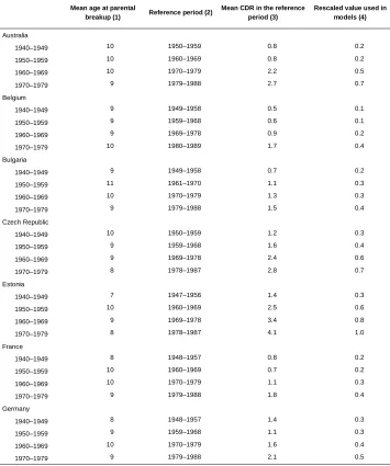
Appendix
Table A-1: Construction of the contextual indicator of divorce rate
Mean age at parental
breakup (1) Reference period (2)
Mean CDR in the reference period (3)
Rescaled value used in models (4)
Australia
1940‒1949 10 1950‒1959 0.8 0.2
1950‒1959 10 1960‒1969 0.8 0.2
1960‒1969 10 1970‒1979 2.2 0.5
1970‒1979 9 1979‒1988 2.7 0.7
Belgium
1940‒1949 9 1949‒1958 0.5 0.1
1950‒1959 9 1959‒1968 0.6 0.1
1960‒1969 9 1969‒1978 0.9 0.2
1970‒1979 10 1980‒1989 1.7 0.4
Bulgaria
1940‒1949 9 1949‒1958 0.7 0.2
1950‒1959 11 1961‒1970 1.1 0.3
1960‒1969 10 1970‒1979 1.3 0.3
1970‒1979 9 1979‒1988 1.5 0.4
Czech Republic
1940‒1949 10 1950‒1959 1.2 0.3
1950‒1959 9 1959‒1968 1.6 0.4
1960‒1969 9 1969‒1978 2.4 0.6
1970‒1979 8 1978‒1987 2.8 0.7
Estonia
1940‒1949 7 1947‒1956 1.4 0.3
1950‒1959 10 1960‒1969 2.5 0.6
1960‒1969 9 1969‒1978 3.4 0.8
1970‒1979 8 1978‒1987 4.1 1.0
France
1940‒1949 8 1948‒1957 0.8 0.2
1950‒1959 10 1960‒1969 0.7 0.2
1960‒1969 10 1970‒1979 1.1 0.3
1970‒1979 9 1979‒1988 1.8 0.4
Germany
1940‒1949 8 1948‒1957 1.4 0.3
1950‒1959 9 1959‒1968 1.1 0.3
1960‒1969 10 1970‒1979 1.6 0.4
Table A-1: (Continued)
Mean age at parental
breakup (1) Reference period (2)
Mean CDR in the reference period (3)
Rescaled value used in models (4)
Hungary
1940‒1949 9 1949‒1958 1.3 0.3
1950‒1959 8 1958‒1967 1.9 0.5
1960‒1969 9 1969‒1978 2.4 0.6
1970‒1979 9 1979‒1988 2.7 0.7
Italy
1940‒1949 7 1947‒1956 0.0 0.0
1950‒1959 10 1960‒1969 0.0 0.0
1960‒1969 10 1970‒1979 0.3 0.1
1970‒1979 10 1980‒1989 0.3 0.1
Lithuania
1940‒1949 6 1946‒1955 0.3 0.1
1950‒1959 8 1958‒1967 1.0 0.2
1960‒1969 9 1969‒1978 2.6 0.6
1970‒1979 8 1978‒1987 3.2 0.8
Netherlands
1940‒1949 8 1948‒1957 0.6 0.1
1950‒1959 10 1960‒1969 0.5 0.1
1960‒1969 11 1971‒1980 1.4 0.3
1970‒1979 9 1979‒1988 2.2 0.5
Norway
1940‒1949 10 1950‒1959 0.6 0.2
1950‒1959 10 1960‒1969 0.7 0.2
1960‒1969 10 1970‒1979 1.3 0.3
1970‒1979 10 1980‒1989 1.9 0.5
Romania
1940‒1949 8 1948‒1957 1.4 0.4
1950‒1959 9 1959‒1968 1.5 0.4
1960‒1969 9 1969‒1978 1.0 0.2
1970‒1979 10 1980‒1989 1.5 0.4
Notes:(1) is the average age at parental breakup of the GGS respondents in each country and cohort combination whose parents broke up before their 18th birthday. The following formula was used to compute values in column 4: (4) = ((3)-min(3))/(max(3)-min(3)).
Table A-2: Construction of the contextual indicator of educational expansion
% with tertiary education Rescaled value used in models
Australia
1940‒1949 23 0.5
1950‒1959 31 0.7
1960‒1969 31 0.7
1970‒1979 36 0.9
Belgium
1940‒1949 20 0.4
1950‒1959 25 0.5
1960‒1969 33 0.8
1970‒1979 41 1.0
Bulgaria
1940‒1949 17 0.3
1950‒1959 22 0.4
1960‒1969 23 0.5
1970‒1979 24 0.5
Czech Republic
1940‒1949 10 0.1
1950‒1959 12 0.1
1960‒1969 14 0.2
1970‒1979 13 0.2
Estonia
1940‒1949 29 0.6
1950‒1959 36 0.9
1960‒1969 32 0.7
1970‒1979 28 0.6
France
1940‒1949 15 0.2
1950‒1959 19 0.3
1960‒1969 24 0.5
1970‒1979 39 0.9
Germany
1940‒1949 23 0.5
1950‒1959 26 0.6
1960‒1969 27 0.6
Table A-2: (Continued)
% with tertiary education Rescaled value used in models
Hungary
1940‒1949 14 0.2
1950‒1959 16 0.2
1960‒1969 18 0.3
1970‒1979 19 0.3
Italy
1940‒1949 7 0.0
1950‒1959 11 0.1
1960‒1969 12 0.1
1970‒1979 15 0.2
Lithuania
1940‒1949 17 0.3
1950‒1959 24 0.5
1960‒1969 22 0.4
1970‒1979 35 0.8
Netherlands
1940‒1949 24 0.5
1950‒1959 29 0.6
1960‒1969 30 0.7
1970‒1979 35 0.8
Norway
1940‒1949 23 0.5
1950‒1959 30 0.7
1960‒1969 34 0.8
1970‒1979 40 1.0
Romania
1940‒1949 8 0.0
1950‒1959 10 0.1
1960‒1969 10 0.1
1970‒1979 13 0.2