University of New Orleans University of New Orleans
ScholarWorks@UNO
ScholarWorks@UNO
University of New Orleans Theses and
Dissertations Dissertations and Theses
5-20-2005
A Comparative Analysis of the Subsurface Stratigraphic
A Comparative Analysis of the Subsurface Stratigraphic
Framework to the Geomorphic Evolution of the Caillou Bay
Framework to the Geomorphic Evolution of the Caillou Bay
Headland, South-Central Louisiana
Headland, South-Central Louisiana
Elizabeth Mary Petro
University of New Orleans
Follow this and additional works at: https://scholarworks.uno.edu/td
Recommended Citation Recommended Citation
Petro, Elizabeth Mary, "A Comparative Analysis of the Subsurface Stratigraphic Framework to the Geomorphic Evolution of the Caillou Bay Headland, South-Central Louisiana" (2005). University of New Orleans Theses and Dissertations. 241.
https://scholarworks.uno.edu/td/241
This Thesis is protected by copyright and/or related rights. It has been brought to you by ScholarWorks@UNO with permission from the rights-holder(s). You are free to use this Thesis in any way that is permitted by the copyright and related rights legislation that applies to your use. For other uses you need to obtain permission from the rights-holder(s) directly, unless additional rights are indicated by a Creative Commons license in the record and/or on the work itself.
A COMPARATIVE ANALYSIS OF THE SUBSURFACE STRATIGRAPHIC FRAMEWORK TO THE GEOMORPHIC EVOLUTION OF THE CAILLOU BAY
HEADLAND, SOUTH-CENTRAL LOUISIANA
A Thesis
Submitted to the Graduate Faculty of the University of New Orleans
in partial fulfillment of the requirements for the degree of
Master of Science in
The Department of Geology and Geophysics
by
Elizabeth M. Petro
B.A. LaSalle University, 2002
Table of Contents
List of Figures …..……….iv
Abstract ….…..……….……….vi
Chapter 1 .……….………..1
Introduction ………...1
Significance ………...3
Applied Considerations ……….3
Theoretical Considerations ………....4
Study Focus and Goals ………..5
Chapter 2 .………..7
Background ………...7
Study Area ……….7
Late Holocene Mississippi River Delta Plain Development ….7 The Caillou Bay Headland Development ………..8
Deltaic Cycle ……….8
Deltaic Depositional Environments ……….………...10
Mississippi River Delta Barrier Island Formation ……….11
Delta Plain Subsidence ……….12
Compaction Studies ………..13
Land Loss in the Caillou Bay Headland Area ………..15
Chapter 3 .……….17
Methods ………17
Stratigraphic Framework ………..17
R/V Greenhead Vibracore Platform ……….19
R/V Gilbert Vibracoring Platform ………20
Core Preparation ………...21
Core Description Technique ……….22
Photography ………..23
Radiocarbon Dating ………..23
Results ………...24
Stratigraphic Framework ………...24
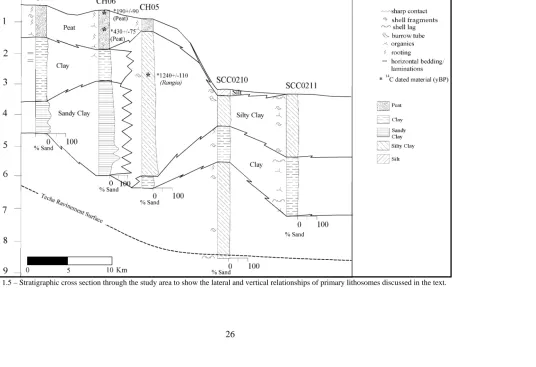
Stratigraphic Cross Section A-A’ ………..25
Stratigraphic Cross Section B-B’ ………...27
Stratigraphic Cross Section C-C’ ………...27
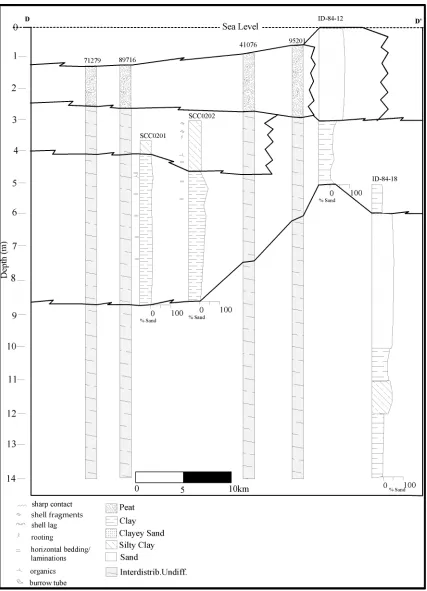
Stratigraphic Cross Section D-D’ ………..29
Stratigraphic Cross Section E-E’ ………...29
Lithosome Contour Maps ………..32
Discussion ………..35
Stratigraphic Cross Section A-A’ ………..35
Stratigraphic Cross Section B-B’ ………...35
Stratigraphic Cross Section C-C’ ………...35
Stratigraphic Cross Section D-D’ ………..36
Stratigraphic Cross Section E-E’ ………...36
Chapter 4 .………...42
Map Preparation ………42
1863 Map ………...44
1895 Map ………...47
1956 Map ………...49
1983 Map ………...52
2002 Map ………...54
Land Loss Map Production ………56
Results ………56
Land Loss Totals ………57
Land Loss Determination ………...57
Discussion ………..61
Map Evaluation ………..61
Comparison of Change: 1863-1895 ………...61
Comparison of Change: 1895-1956 ………...62
Comparison of Change: 1956-1983 ………...62
Comparison of Change: 1983-2002 ………...62
Chapter 5 .………...64
Discussion and Conclusions ………...64
Percent Land Loss versus Lithosome Thickness ………...64
Chart 1: Percent Land Loss versus Lithosome Thickness- Time Interval A (1895-1956) ……….65
Chart 2: Percent Land Loss versus Lithosome Thickness- Time Interval B (1956-1983) ……….65
Chart 3: Percent Land Loss versus Lithosome Thickness- Time Interval C (1983-2002) ……….66
Summary ………81
Works Cited……….83
Appendices………..85
List of Figures
1.1 – Study area map with major bayous and relict shorelines identified.
1.2 - Study area map with major relict deltaic lobes identified.
1.3 - Soil subsidence potential map.
1.4 – Study area map with locations of cores obtained and cross section locations.
1.5 - Cross section A-A’.
1.6 - Cross section B-B’.
1.7 - Cross section C-C’.
1.8 - Cross section D-D’.
1.9 - Cross section E-E’
1.10 - Cross section A-A’ (stylized).
1.11 - Cross section B-B’ (stylized).
1.12 - Cross section C-C’ (stylized).
1.13 - Cross section D-D’ (stylized).
1.14 - Cross section E-E’ (stylized).
1.15 – Digital image produced from 1863 paper map.
1.16 – Digital image produced from 1895 paper map.
1.17 – Digital image produced from 1956 paper map.
1.18 – Digital image produced from 1983 paper map.
1.19 – Digital image produced from 2002 digital map.
1.20 – Land loss map 1895-1956.
1.21 – Land loss map 1956-1983.
1.23 – Peat lithosome thickness v. 1895-1956 land loss map.
1.24 - Peat lithosome thickness v. 1956-1983 land loss map.
1.25 - Peat lithosome thickness v. 1983-2002 land loss map.
1.26 – Clay lithosome thickness v. 1895-1956 land loss map.
1.27 - Clay lithosome thickness v. 1956-1983 land loss map.
1.28 - Clay lithosome thickness v. 1983-2002 land loss map.
1.29 – Silty Clay lithosome thickness v. 1895-1956 land loss map.
1.30 – Silty Clay lithosome thickness v. 1956-1983 land loss map.
1.31 – Silty Clay lithosome thickness v. 1983-2002 land loss map.
1.32 – Sandy Clay lithosome thickness v. 1895-1956 land loss map.
1.33 – Sandy Clay lithosome thickness v. 1956-1983 land loss map.
1.34 – Sandy Clay lithosome thickness v. 1983-2002 land loss map.
1.35 – Percent land loss v. lithosome thickness plots.
Abstract
Studies have documented spatially and temporally variable rates of surface subsidence
across the Mississippi River delta plain of Louisiana. Variations in patterns and rates of delta
plain subsidence may reflect subsurface distribution of compaction-prone lithosomes.
This research investigates historical changes in the surface geomorphology of the Caillou Bay
headland in relation to the distribution of subsurface lithosomes. The stratigraphic framework
was developed for the headland, and lithosomes were identified to establish the distribution of
different sedimentary units. The geomorphic evolution as indicated by maps was then evaluated
in order to locate patterns of shoreline change and wetland loss for the headland. Land loss maps
developed were overlain on lithosome contour maps to calculate amounts of land loss overlying
each lithosome contour interval. Analysis of results revealed that land loss was not uniform
throughout the headland and that land loss patterns for several time periods varied as a function
Chapter 1
Introduction
The modern Mississippi River delta plain of southern Louisiana has been built
throughout the last 6,000 years by the deposition of sediments from the Mississippi River
and its associated distributaries (Frazier, 1967). During this time the delta plain was
deposited as multiple temporally and spatially distinct deltaic progradational events
occurred. These progradations successively expanded the deltaic plain and the Holocene
sedimentary package. As each delta lobe prograded, the river gradient decreased.
Through time this would force the river distributary to avulse and relocate, occupying
another channel with a higher basinward gradient. This delta switching cycle created four
distinct deltaic complexes, each one consisting of multiple overlapping delta lobes
(Penland et al., 1987) (Fig. 1.1). Each of the lobes within a deltaic complex consisted of
a network of distributaries that were flanked by natural levees, interdistributary bays,
crevasse splays, subdeltas, marsh platforms, and swamps. Progradation is the
fundamental process contributing toward the formation of a deltaic headland; once
abandoned these headlands became sites of transgressive reworking and are modified by
marine processes such as tides and waves. Although some of the processes involved in
headland formation and evolution are understood reasonably well (e.g. progradation and
marine reworking) there are other contributing factors, such as compaction-driven
subsidence, that remain poorly qualified. Previous researchers have suggested that some
trends in land loss and change are the result of the distribution of these compactable
The intent of this research is to investigate the role of shallow subsurface
compaction in headland geomorphic evolution. The study area for this research is the
Caillou Bay headland, located in south-central Louisiana (Figure 1.1). The main
objectives of this research are to: 1) determine the patterns of erosion along the southern
most extent of the Caillou Bay Headland and, 2) compare these patterns of geomorphic
change to the distribution of shallow, subsurface sedimentary bodies.
Significance
The stratigraphic framework and distribution of lithosomes within deltaic
headlands reflects variability in the distribution of deltaic subenvironments that are
formed during progradation. Because lithosomes may exhibit variation in their
sedimentology the expectation is that they will be susceptible to different rates of
compaction during burial and dewatering. Conceptually, this implies that areas of the
headland may subside at different rates, leading to different rates of relative sea-level
rise, inundation, reworking, and the ultimate conversion of marsh platform to open water.
Applied Considerations
Coastal land loss across the delta plain is an issue of particular concern in
southeastern Louisiana (Barras et al., 2003). This loss is a result of naturally occurring
geologic processes, such as subsidence and sea-level rise, as well as substantial
anthropogenic modifications, such as access canal and levee construction. Interior marsh
platform loss and shoreline change are both recorded as land loss. Interior marsh
platform loss is thought to be due primarily to subsidence and anthropogenic
modifications, whereas shoreline change has primarily occurred as a function of sea level
km2 per year along some sections of the coastal zone have been presented (Barras et al.,
2003). Rates of land loss have not remained temporally constant nor are they spatially
uniform along the coast (Britsch and Dunbar, 1993). This variability has made
determining patterns of erosion difficult. The goal of the work is to provide needed
insight into the extent that differential compaction of lithosomes, with varying degrees of
compaction potential, influence the geomorphic evolution of a delta headland. A
thorough understanding of this has both theoretical and applied importance.
One important aspect of this research is to develop an understanding of the
stratigraphic architecture underlying the Caillou Bay Headland. Developing the
stratigraphic framework of the headland will aid in determining its transgressive history
and evolution. Subsequently, this can help in predicting how coastal restoration projects
may perform over time. Differential compaction is one of several variables that affect the
evolution of the headland. The utility of establishing a better understanding between the
subsurface geology and the surficial geomorphology is that an understanding of the
overall transgressive development of the headland will be developed. This will then aid
in the development of models that predict future coastal land lost in terms of the nature,
rate, and location of headland retreat.
Theoretical Considerations
Determining the distribution of these facies is significant in discerning the
influence of delta lithosome distribution on subsequent deltaic sedimentation. For
example, Fisk (1955) suggested that variability in thickness, extent, and stratigraphy of
deltaic depocenters is influenced by water depths in which deltaic progradation takes
development of thin, laterally extensive deltaic depocenters. Alternatively, more
substantial accommodation space will result in a more laterally restricted but potentially
overall thicker depocenter. Because of the overlapping nature of deltaic lobes
stratigraphically higher deltaic deposits may have been influenced by the topography of
underlying depocenters. Topography of the subjacent depocenter partially develops in
response to compaction, which is in turn influenced by the composition of the
stratigraphy within the underlying deposit. Consequently, specific knowledge of the
processes that control the generation of accommodation space can assist in determining
the likely location of subsequent delta depocenters. Developing a detailed picture of the
shallow stratigraphy of a deltaic headland may provide insight as to how complex
reservoir systems form in response to differential rates of compaction.
Study Focus and Goals
This study investigates the question of whether variable compaction of different
sedimentary bodies within the Caillou Bay Headland has influenced the
post-progradational evolution of the headland.
Two primary datasets, a subsurface framework geology evaluation and an
evaluation of the geomorphic evolution of the headland will be assembled. The first
dataset consists of previously acquired cores within a large database of archived core data
at UNO, as well as cores that were collected specifically for this study. Collectively,
these cores will be used to create cross sections for a variety of locations on the headland
and aid in the identification of primary lithosomes. Lithosomes are identified as
character. These characteristics include grain size and distribution, sediment color, and
the style of bedding. The intent is to identify the various sedimentary types in order to
determine the distribution of compactable lithosomes. These sedimentary units will be
used to develop isopach maps depicting unit thickness.
The second dataset is a collection of maps for the time period 1863 to present.
The utility of these maps is that they provide a historical record of the headland size and
geomorphology; comparison of these maps to one another allows for an evaluation of the
geomorphic evolution of the Caillou Bay headland and documentation of the distribution
and rate of headland evolution within the historic record that is available. The results
constitute a primary component of this research and the ability to identify areas of
significant land loss in the study area. The intent is to use these two datasets in
conjunction with one another and evaluate whether any correlation exists between the
subsurface sediment distributions, as indicated by the core dataset, and the historical
Chapter 2
Background
This study of the Caillou Bay headland focuses on defining the relationship
between the stratigraphic framework and the historical (1895 to 2002) geomorphic
evolution. The two main components of the research consist of developing a
stratigraphic framework of the headland and compiling a quantitative evaluation of land
loss through time across the entirety of the headland.
Study Area
The Caillou Bay headland is located in south-central Louisiana, approximately 75
km south of Houma, Louisiana (Figure 1.1). The study area is bounded along the north
by the northern shore of Caillou Lake, in the south by the Isle Dernieres, on the west by
the mouth of Oyster Bayou, and along the east by the eastern edge of Timbalier Island. A
generally north-to-south network of active and semi-active bayous trend across the study
area. Several of these are thought to have been active for at least the last 3,000 yrs BP
(Penland et al., 1988), although more recently carrying substantially less flow than at
previous times.
Late Holocene Mississippi River Delta Plain Development
The late Holocene Mississippi River delta plain developed during the current sea
level high-stand, approximately 6,000 years B.P. (Fisk, 1944; Frazier, 1967; Penland et
al., 1988). The delta plain consists of five major delta complexes composed of multiple
delta lobes that represent the depocenters of temporally and spatially separate
River. The five distinct delta complexes, in order of decreasing age are: Maringouin –
Teche, St. Bernard, Lafourche, Plaquemines-Balize, and Atchafalaya complexes (Frazier,
1967).
Caillou Bay Headland Development
The Caillou Bay headland is the third lobe of the Lafourche delta complex and
was active between approximately 910 to 420 years B.P. (Penland et al., 1987). The
headland was built by deposition from four primary distributaries: Bayou Grand Caillou,
Bayou Chauvin, Four Point Bayou, and Bayou Sale (Penland et al., 1987). In general, a
deltaic headland consists of a complex assemblage of facies constructed during
progradation (Frazier, 1967) (Figure 1.2). Several factors influence deltaic progradation.
The sediment load of the river, rates and patterns of subsidence, and sea-level change
influence the overall thickness and lateral extent of facies within the headland.
Transgressive reworking due to sea level rise and subsidence can alter the sediment
distribution post deposition.
Deltaic Cycle
In general the Caillou Bay headland developed within the conceptual framework
known as the delta cycle. The delta cycle describes the progradation and subsequent
reworking of a deltaic headland that becomes abandoned and starved of river supplied
sediment. Delta lobe progradation begins with the entrainment of a distributary system
between levees built through time during episodes of river flooding. Progradation
proceeds as deltaic facies accumulate on the shelf. Thick units of prodelta silts and clays,
at the distal edge of the progradational site, accumulate and compact where the finer
vertically. A complex network of bayous, natural levees, swamps, and marsh develop
through time. Sediment continues to accrete and the vertical gradient decreases. When
the gradient decreases sufficiently the river avulses and changes geographic position to
where the gradient is steeper, resulting in the initiation of a new delta cycle (Fisk, 1944;
Kolb and Van Lopik, 1958, Coleman and Gagliano, 1964). During the Holocene
repeated occurrence of these processes has resulted in the formation of the modern
Mississippi River delta plain.
Figure 1.2 – Satellite image (2002) with Frazier’s Lafourche delta lobes plotted to show the extent of deposition associated with the progradation of the deltas. Most of the project area is within the area covered by lobe 14, thought to have been deposited between 900-100 B.P. (Frazier, 1967).
700000 680000
660000 720000 740000 760000
3300000 3280000 3260000 3240000 3220000 N
0 5 10 20 Km
Lobe 14 Lobe 6 C o o rd ia n a te s (U T M Z o n e 1 5 )
Deltaic Depositional Environments
The action of the deltaic cycle has resulted in the construction of the modern
Mississippi River delta plain. A cycle is composed of several sedimentary units: prodelta
silts and clays, shelf shell and clay beds, delta front silts and clays, interdistributary bay
clays and silty clays, natural levee silty clays and sands, and swampy organic clays and
peats (Coleman and Gagliano, 1964).
Various researchers have identified and described prodelta deposits. They have
been described as silty clays similar to those found within a deltaic-plain complex and
form thick, widespread units around the front of the deltaic-plain facies (Fisk and
McFarlan, 1955). They have also been described as thick silty clays with burrowed and
nonburrowed zones containing rhythmic laminations of silt and clay and colors (Coleman
and Gagliano, 1964), and as homogenous fat clay sequence from fine to coarse (Kolb and
Van Lopik, 1958).
Interdistributary deposits have been identified and described as bay clays and silty
clays with storm debris inclusions, shell fragments, burrows, and plant remains (Coleman
and Gagliano, 1964). They have also been described as mostly inorganic fat clays and
silt (Kolb and Van Lopik, 1958).
Natural levee deposits are identified and described as silts and clays (Fisk and
McFarlan, 1955). They have also been described as fat clay and silt accumulations
oxidized to a tan or reddish (Kolb and Van Lopik, 1958), and as silty clays (Coleman and
Marsh deposits are identified and described as both organic and nonorganic. The
organic component has been described as containing high organic content with roots and
wood fragments (Fisk and McFarlan, 1955), as highly organic clays and peats (Coleman
and Gagliano, 1964), and as brown to black fibrous or felty masses of partly decomposed
remains of plant material and organic float material from hurricane deposits (Kolb and
Van Lopik, 1958). The inorganic component of the marsh deposit has been described as
largely silty clays (Fisk and McFarlan, 1955), and as clays silts and fine sands (Kolb and
Van Lopik, 1958).
Mississippi River Delta Plain Barrier Island Formation
Barrier island formation within the Mississippi River delta plain initiates with
distributary abandonment and subsequent reworking of the abandoned headland by
marine processes. The model for barrier island formation is a three-step process; (1) the
erosion of the headland and the formation of flanking barriers, (2) the development of a
transgressive barrier island arc, (3) and the formation of an inner-shelf shoal (Penland et
al., 1988).
In the first stage, marine processes begin to rework the abandoned deltaic
headland. Main distributary deposition ceases so there is limited sediment to fill in the
accommodation space created by the subsiding headland. At this stage the transgressive
headland consists of several components; an erosional headland, a beach, flanking spits
and barrier islands, tidal inlets and deltas, restricted interdistributary bays, and a
transgressive sand sheet (Penland et al., 1988). Longshore currents and tides transport
sand that augments the flanking barrier islands. Sediment on the seaward fringe of the
restricted interdistributary bays in response to the initial rapid subsidence (Penland et al.,
1988). Tidal inlets and associated tidal delta deposits form as barrier breaching occurs.
Increasing bay-area causes an increasing number of tidal prisms to form inlets which
allow these bays to remain open (Penland et al., 1988).
The second stage of the process consists of continued transgressive reworking of
the erosional headland, and mainland detachment forming a barrier island arc, tidal inlets,
lagoons, and an inner-shelf sand sheet (Penland et al., 1988). The erosional headland and
flanking barrier islands constructed during stage one detach and form a transgressive
barrier island arc. Storm events cut through the islands forming tidal inlets. The
restricted interdistributary bay area opens up with the detachment of the barrier islands
and tidal exchange with the gulf becomes a dominant process. Sand eroding away from
the shoreline and the barrier islands is deposited on the shoreface to form transgressive
inner shelf sand sheet (Penland et al., 1988).
The third and final stage of the process consists of the development of inner shelf
shoals. As a result of RSL and marine reworking the barrier island is inundated. The
components comprising this stage include shoal crest, shoal front, shoal base, sand sheet,
and maximum shoreline (Penland et al., 1988). The shoal crest, front, and base are all
reworked remnants of the barrier island arc. Reworking and landward migration of the
shoal continues after submergence (Penland et al., 1988).
Raccoon Island, Whiskey Island, and Trinity Island of the Isles Dernieres island
arc (stage 2) of Penland et al., (1988) are the primary barrier islands located in the study
area (Figure 1.11).
The Mississippi River delta plain is actively subsiding as a result of numerous
contributing mechanisms (e.g. compaction, faulting, regional isostatic adjustment)
(Figure 1.3) (Roberts et al., 1993; Kulp et al., 2002). Subsidence rates have been
previously determined using age-depth relationships of radiocarbon-dated peat deposits
located in the subsurface of the study area. These data yield subsidence rates that range
between approximately 33.4cm/100 yr to 39.6 cm/100 yrs (Roberts et al., 1994). Roberts
et al. (1994) also noted that subsidence patterns closely follow the distribution of
Holocene deposit thickness; the highest subsidence rates are located above the thickest
Holocene strata because of greater compaction potential in the thick, highly compactable
sediments of the Holocene interval.
Compaction Studies
In this study, the compaction of sediment is considered to be the most significant
component of marsh-platform subsidence in the study area (Figure 1.3).
The most widely accepted theory of one-dimensional consolidation was
developed by Terzaghi (1943). Terzaghi recognized that when sediments are
compressed, water is released and pore space diminishes (Clayton et al., 1995). Under
natural conditions compaction occurs because of sediment dewatering that occurs as
strata are buried by overlying sediment.
Compaction can be simply defined as a “change in sediment dimensions during
burial (Giles et al., 1998). Initial compaction is the result of sediment loading, which
leads to a vertical reduction in sediment volume (Giles et al., 1998). Thus as sediment
accumulates and becomes buried, water flows out of the sediment, pore space is reduced,
Figure 1.3 - Soil subsidence potential map showing the distribution of subsidence likelihood across a portion of the south-central coastal zone (adapted from Louisiana State Planning Office, 1976). The box outlines the study area of this project. Note: the soils of the study area are mapped as high compaction potential if drained, soils in this area consist of more than 130-cm thick organic material.
compaction. Coarser grained sediments such as sand have been observed to be more
resistant to compaction than finer grained sediments such as clay (Holbrook, 2002).
The compaction rate of sediments is highly variable, so previously determined
determined compaction indices for various deltaic facies in the Terrebonne region.
Keucher (1994) found that the most compactable facies were finer-grained, such as peats
and clays; he found that the least compactable facies were coarse-grained such as silt.
Land Loss in the Caillou Bay Headland Area
Land Loss on the Mississippi River delta plain is a topic of particular concern to
those living and working in Southeastern Louisiana. Current estimates place land loss in
some areas as high as 62 km2 per year (Barras et al., 2003). This land loss has both
natural and anthropogenic origins. The natural causes include subsidence, herbivory, and
storm and wave action (Kindinger et al., 2002). Anthropogenic causes include direct
removal of land for the purpose of channel and pond construction, borrow pits, and
altered hydrology (Kindinger et al., 2002)
A significant amount of research has evaluated land loss on the Mississippi River
delta plain (Barras et al., 2003; Britsch and Dunbar, 1993; Gagliano et al., 1981). In a
recent study (Barras et al., 2003) several land loss trends were noted. From 1956-1978
large areas of marsh have converted to open water, and from 1978-1990 this trend
continued at a less rapid rate (Barras et al., 2003). During the last decade, however, the
primary mode of land loss has been the formation of small ponds in the interior marsh
and shoreline erosion. In the Terrebonne region, where this study was conducted,
significant erosion continues for the 1990–2000 interval. Most of the recent loss is
occurring in areas that have already undergone the most significant land loss (Barras et
al., 2003). Shoreline erosion and interior marsh pond formation are the most significant
2004). Observed land gain can possibly be attributed to the movement of detached, or
Chapter 3
Methods
Stratigraphic Framework
A primary objective of this investigation is to establish the fundamental
stratigraphic framework of the Caillou Bay Headland. The goal is to identify and map
the primary subsurface lithofacies. The UNO Coastal Research Laboratory (UNO CRL)
core database and a United States Army Corp of Engineers (USACE) database were
searched to determine whether any cores had been previously obtained within the study
area. For each core the database contains a physical description sheet, and in many
instances grain size analysis data and core photography. A total of ten cores from the
UNO database and thirteen cores from the USACE database were identified as having
potential value to the project. The cores were loaded into a GIS platform and plotted to
visualize the distribution of the cores.
The distribution of the preexisting cores was used to develop a strategy for
obtaining new cores, thereby avoiding redundancy, obtaining data where cores were
missing and increasing the overall number of cores available for a stratigraphic analysis
of the headland. For this purpose a team of field geologists, as part of a larger project on
delta plain subsidence collected a total of 26 cores within the study area (Figure 1.4).
Core locations were located by plotting target sites on a base map of the area. Slight
adjustments, generally less than 25 m offset, to the locations of cores were made in the
field when obstacles such as oil and gas pipelines, and private property, or other
Figure 1.4 – Basemap showing the locations of cores and cross sections used in this study to characterize the framework stratigraphy of the Caillou Bay headland.
321000 322000 323000 324000 325000
690000 700000 710000 720000 730000 740000 750000
57037 SCC0204 101204 SCC0205 SCC0206 CH13 7270 CH12 P-1-90 WW-5041z FC-2 SCC0201 SCC0202 41076 95201 ID-84-12 ID-84-18 59894 SCC0207 SCC0208 26320 SCC0212 77181 CH03 CH04 FPB-10 78097 SCC0211 SCC0210 SCC0209 CH11 CH10 BJ-1 CH05 CH06 CH07 CH08 130615 DL-3 120012 CH09 113021 WW-5032z FL-7 CH01 159026 CH02 80606 71279 89716 128322 35298 C-13 40509 SCC0203b 62945 55709 38941 52443 A A' B B' C C' D D' E E'
0 10 20 Km
N
Coordinates (UTM Zone 15)
C o o rd in at es ( U T
M Z
o n e 1 5 )
UNO Coastal Research Lab Cores Summer 2003 USGS Cores Summer 2003
USGS Auger Cores Summer 2003 USACE Database cores Penland et. al. cores 1987
Cross section lines
Raccoon Island Whiskey Island
Trinity Island
Timbalier Island
Gulf of Mexico
Timbalier Bay
Caillou Bay Lake Merchant Lost Lake
Two distinctly different vibracoring rigs were used to obtain the cores during the
2003 summer field season. A field team on the UNO R/V Greenhead acquired 13 cores
located in areas where the water was less than 1.5 m deep. In locations where the water
depth exceeded 1.5 m the USGS R/V Gilbert was used as a vibracoring platform,
resulting in the acquisition of an additional 13 cores. Vibracore sites were reached using
the geographic coordinates acquired from the core database and recorded in a logbook.
R/V Greenhead Vibracore Platform
The vibracoring system used by the UNO CRL consists of a tripod mounted to a
flat bottom boat. The tripod is positioned over a moon pool in the hull of the R/V
Greenhead, which allows for access to the water below. A 9-meter long aluminum tube
with an approximately 7.5 cm diameter is inserted vertically into the center of the tripod.
A weighted vibracore head is attached to the aluminum pipe and tightened in place. A
cable to a gas-powered combustion engine that powers the system is connected to the
head. The motor speed is adjusted until a vibration frequency is attained that liquefies the
underlying sediments and allows the aluminum tubing to penetrate into the subsurface.
The vibration frequency must be adjusted when the tubing encounters strata that are
compositionally different or have undergone different degrees of compaction.
Vibracoring continues until a depth is reached at which further penetration cannot be
made, even when additional pressure is applied and when the frequency of vibration is
altered by varying the engine speed. Penetration can be interrupted when coarser units
such as sand or shell lag are encountered. Care was used when additional pressure was
A metric tape measure was used to record water depth at the site and the depth to
the top of the sediment water interface inside the penetrated core. This information was
used later to calculate the magnitude of sediment column compaction that occurred
during the vibracoring process. This value is important when constructing cross sections
to accurately determine the original thickness of sediment units. It is crucial to determine
if the core extracted replicates the strata, or if excess compaction must be accounted for.
After these measurements have been made any excess tubing is cut off and properly
discarded. In order to extract the core intact and within the tubing, water is poured into
the top of the core barrel and a plug is inserted and tightened in the top of the tubing to
create a vacuum within the tube above the sediment section retained within the core
barrel. A hook attached to a steel cable is fastened to the barrel and a hand winch is used
to extract from the ground the aluminum tube containing the core. After the core barrel
has been removed from the subsurface, the top and bottom of the core is sealed with a
plastic cap and taped at both ends to hold the sediment sample in place within the core.
The total core length is then measured, the core is labeled, and the top and bottom of the
core is clearly marked before being transported back to a laboratory for analysis.
R/V Gilbert Vibracoring Platform
The USGS vibracoring system operates off the R/V Gilbert and is capable of
obtaining cores in as much as 37 meters of water depth. A Global Positioning System
(GPS) was used to position the rig at the preselected core sites and the core locations
were recorded in a logbook. The R/V Gilbert vibracoring system consists of a
stationary aluminum mast attached to a 400-lb rectangular frame. Two electric
compressors drive a 6-meter long aluminum tube with an approximately 7.5 cm diameter
into the subsurface. A check-ball valve is located on the vibracore head and is attached to
the top of the core to act as a vacuum seal. This is combined with a core catcher
consisting of collapsible brass at the base of the core. This helps to retain the sediment in
the core when it is extracted from the seabed. The core is extracted using an electric
winch that pulls a braided wire cable attached to the vibracore head. Similar to the
procedure used on the R/V Greenhead, the core was sealed with a plastic cap and tape at
both ends. The core was then measured, labeled, and the top and bottom of the core
clearly marked before being transported back to a UNO laboratory for analysis.
Core Preparation
Cores acquired in the field were then brought back to the UNO-Chevron Earth
Science laboratory and prepared for visual description, sampling, and photography. In
the laboratory the cores were marked in two-meter increments along the length and cut
into more manageable sections at these marks. The exposed ends where then resealed
with a plastic cap and tape. A circular saw was used to make two opposing cuts
vertically along the length of the cores. A thin wire was then run down the center of the
cores along these length-wise cuts and the cores were split into two even halves. The half
with the least amount of wire marks was designated the archival half of the core, whereas
the other half was designated the work half. The work half was set aside for grain size
sampling and the collection of material, such as peat and shells that could be radiocarbon
to remove the top layer of sediment that may have been smeared by the wire. Core
halves that had been smoothed were then visually described.
Core Description Technique
A visual description was completed on each core (individual description sheets
are included in Appendix A). Standard templates designed by Coastal Research
Laboratory (CRL) researchers were used to record the data. The cores were described
from top to bottom. The approach employed in this study was to first make note of major
sedimentary units by looking for changes in lithology, erosional surfaces, significant
change in sediment color, or changes in sedimentary structures. These individual units
were then described in detail to provide an in depth description of the core.
The approach was to first determine the textural classification of the sediments.
For this the Udden-Wentworth scale was relied upon. The classifications used for the
cores described were clay (<1/256 mm), silt (1/256 to 1/16 mm), fine sand (1/8 to 1/4
mm), medium sand (1/4 to 1/2 mm), and coarse sand (1 to 2 mm) (Wentworth, 1922).
Percent sand was then identified, from zero to one hundred percent. Additional physical
characteristics that were described for each previously determined sedimentary interval
were color, style of bedding, bed thickness, percent shell material, percent organic
material, and percent bioturbation. Stratification types that were noted included wavy,
flaser, lenticular, massive bed, inclined, and horizontally laminated. A detailed physical
Photography
Upon completion of the core description, photographs were taken of each core.
These pictures are archived at UNO within the CRL core database. For the first set of
photographs, the two-meter increments of each core were photographed in 40-cm
increments. A cardboard template with a scale and project title was created and placed
over each increment. These detailed photographs are helpful when cross checking the
core description sheets after the original cores have aged and desiccated. The two-meter
core sections were then cut into one-meter sections and placed on a rack with a scale in
order to obtain a whole-core photograph.
Radiocarbon Dating
Four peat samples and two whole Rangia cuneata shell specimens were sent to
the University of Arizona (UA) Isotope Geochemistry Laboratory for radiocarbon dating
to aid with stratigraphic analysis. Before the samples were sent to UA they were
prepared by drying them in an oven at 30° C for 36 hours as requested by the UA
laboratory. The peats and whole shells were then weighed and this information was
recorded on a data sheet that was additionally submitted with each sample that was sent
to UA.
Peat samples were chosen from cores with thick continuous peat deposits that
contained negligible amounts of clastic material so enough organic material would be
they are not likely to be reworked and thus are assumed in situ. The samples were
wrapped in aluminum foil as specified by the UA laboratory, labeled, and each placed in
individual sealed bags with their corresponding data sheet. They were then shipped to
UA for analysis.
Each sample was dated using the liquid scintillation counting technique. This
process included stable carbon isotopic analysis and calibration. The calibration process
corrects for fluctuations in the amount of radiocarbon present in the atmosphere
throughout time (Stuiver et al., 1998). UA’s calibration curve is based on the known age
of tree rings, corals (independently dated by U-Th) and annually laminated sediments
(Stuiver et al., 1998).
Results
Stratigraphic Framework
A total of 26 new vibracores (Appendix A) were described and incorporated into
the UNO core database. From these cores a total of five stratigraphic cross-sections were
constructed across the Caillou Bay headland to aid in depicting the subsurface geology
(Figure 1.1). The cross sections are constrained by sea level at the top and the Teche
Ravinement surface at the base of the section as defined by Penland et al., (1987).
The sedimentary units identified in the cores were peat, clay, silty clay, sandy
clay, clayey sand, and sand. Peat units were defined when the organic content of the unit
was greater than 50% organic material, and clays and silty clays were sometimes
interbedded with the organic material. Clay units were defined when the unit was
Stratigraphic cross section A-A’
Stratigraphic cross section A-A’ trends from the North East to the South West
from Moncleuse Bay to South of Oyster Bayou (Figure 1.5). A peat unit tapers from 1.0
meter in thickness at Moncleuse Bay to 0.50 m thick at the southern portion of Caillou
Lake and pinches out over Bayou Grand Caillou. The peat unit contains numerous roots
throughout and has shell fragments near Moncleuse Bay. The peat overlies a clay unit
2.0 m thick that tapers to 1.25 m at the southern portion of Caillou Lake and pinches out.
The clay unit shows horizontal lamination and some organic fragments where it pinches
out. The clay overlies a sandy clay unit that is a 1.0 m thick at Moncleuse Bay and
thickens to 3.0 m where it ends at the southern portion of Caillou Lake. A 4.0-m thick
silty clay unit begins where the clay and sandy clay units end laterally. The silty clay unit
thins to 1.0 m at Caillou Bay and is overlain by a 0.25 m thick silt unit. The silty clay
then thickens to 2.0 m south of Oyster Bayou. The silty clay unit has shell fragments
throughout, and burrow tubes where it is overlain by the silt unit. The silty clay overlies
a clay unit that is 25 cm thick at Bayou Grand Caillou and thickens to 2.0 m south of
Oyster Bayou. The clay unit has shell and organic fragments throughout. Three samples
were obtained from the cores in the cross section for radiocarbon dating, two peat
Stratigraphic cross section B-B’
Stratigraphic cross section B-B’ trends from the North to the South from
Moncleuse Bay to South West of Bay Wilson (Figure 1.6). A 1.0 m thick peat unit
stretches from Moncleuse Bay to Grand Pass Ilettes. The peat thickens to 2.0 m at
Hackberry Lake then thins again until it pinches out at the seaward extent of the
headland. The peat overlies a clay unit approximately 2.0-m thick that extends across the
entire section. The peat has rooting throughout and some shell fragments at the northern
end of the section. The clay thickens to 4.5 m west of Bay Wilson and is overlain by a 50
cm thick silt deposit. It then thins to 2.0 m and is overlain by a clayey sand lens. The
clay is horizontally laminated and there are numerous shell fragments and burrow tubes
west and southwest of Bay Wilson. The clay overlies a sandy clay unit that thickens
from 1.0 m to 2.0 m at Hackberry Lake and thickens again to 3.0 m southwest of Bay
Wilson. The sandy clay is horizontally laminated throughout and there are numerous
shell fragments west and southwest of Bay Wilson.
Stratigraphic cross section C-C’
Stratigraphic cross section C-C’ trends from the north to south from Dulac, LA to
Whiskey Pass (Figure 1.7). A 1.0 m thick peat unit extends the entire length of the
section. The peat unit has abundant rooting. The peat overlies a 2.0-meter thick clay unit
that extends to Charleys Lake where it ends. The there are infrequent organic fragments
and some rooting. The clay overlies a 1.0 m thick sandy clay unit that gradually
increases to 2.0 m then tapers to 1.0 m where it ends at Charleys Lake. There are few
clay at core sites FC-2 and ww-5032z. The sandy and silty clay overlies a clay unit that
is 4.0 m thick and gradually tapers to approximately 3.0 m southwest of Charleys Lake
and abruptly ends. The clay is horizontally laminated and a few shell fragments are
present in the unit. There are three 25 cm sand lenses in the clay unit, one at core site
FC-2, one at FPB-10, and one at CH03. South of Charleys Lake a silty clay unit
underlies the peat unit. The silty clay unit starts at 3.0 m thick and gradually increases to
6.0 m at Whiskey Pass. The unit is horizontally laminated and has sparse shell
fragments. Three samples were obtained from the cores in the cross section for
radiocarbon dating, two peat samples and one articulated shell (Table 1.2).
Stratigraphic cross section D-D’
Stratigraphic cross section D-D’ trends from the north to south from Bay Sale to
Trinity Island (Figure 1.8). A 1.0 meter thick peat unit extends from Bay Sale to Trinity
Island and gradually thickens to 2.0 m. The peat overlies a 1.5 m thick silty clay unit that
ends at Pass la Poule. The unit has sparse organic and shell fragments. The silty clay
overlies a 4.5 m thick clay unit that extends from Bay Sale to Trinity Island and gradually
thins to 3.0 m. The clay unit is horizontally laminated. A 3.0 m thick sand unit overlies
the clay unit at Trinity Island.
Stratigraphic cross section E-E’
Stratigraphic cross section E-E’ trends from the northwest to the southeast from
Cocodrie, LA to Timbalier Island (Figure 1.9). An approximately 2.0 m thick peat unit
extends from Cocodrie to Timbalier Bay, except where it is absent under Bay Chaland.
The peat shows sporadic rooting in the northwest portion of the section. The clay
thick clay unit that thickens gradually to 7.0 m at Bay Chaland. The clay abruptly thins
back to 5.0 m, and then tapers to 1.5 m at Timbalier Island. The clay is horizontally
laminated and contains numerous shell fragments south of Bay Chaland. A 2.0 m thick
silty clay unit begins at Bay Chaland and gradually thickens to 3.5 m. The silty clay unit
is horizontally laminated and numerous shell fragments and shell lags are present north of
Timbalier Island. Two clayey sand lenses containing organic and shell fragments are
present in the silty clay unit at core numbers SCC0206 and SCC0204.
Lithosome Contour Maps
Four contour maps were constructed using the sedimentological data for each
lithosome. Sedimentary units described from the cores were grouped into four lithosome
categories; peat, clay, silty clay, and sandy clay. The contour maps were constructed in
order to evaluate the extent of subsurface lithosomes identified from the cross sections.
The interpolate to raster function within ArcGis 8.3 was used to construct contour maps
with interval values based on lithosome thickness. ArcGis 8.3 provides a variety of
contouring algorithms and each one has a particular use depending upon the character of
the data being contoured. In this case inverse distance weighted (IDW) was chosen. Arc
GIS 8.3 provides three contouring operations, and the IDW best fit the data set
assembled. The Z value chosen was unit thickness, the power selected was four, the
search radius was variable, and the output cell size was designated as three pixels to
Discussion
Five transects were constructed across the headland in order to capture the
stratigraphic framework. Identifying the major lithosomes was necessary in order to
determine were the units of varying compatibility are located.
Stratigraphic cross section A-A’
This section transects Caillou Lake and the seaward marginal marshes southwest
of the lake (Figure 1.10). Underlying Caillou Lake the stratigraphic architecture is
simple, marsh deposit overlying clay that overlies sandy clay. This has been interpreted
to be an interdistributary fill deposit. Towards the seaward marshes however this deposit
abuts a deposit that is interpreted as reworked interdistributary bay clays and silty clays,
due to the presences of several shell lags and organic fragments at depth.
Stratigraphic cross section B-B’
This section is comprised of a simple stratigraphic arrangement of sedimentary
units (Figure 1.11). It lies between Bayou Grand Caillou and Pass de Ilettes. The marsh
deposit extends to the seaward extent of the headland where it pinches out. The marsh
unit overlies a thick clay unit and a thick sandy clay unit. The clay and silty clay units
are interpreted as interdistributary bay fill deposits.
Stratigraphic cross section C-C’
This section transects the center of the headland and ends just north of the Isles
Dernieres (Figure 1.12). In this section two distinct thick clay strata were observed.
interdistributary bay fill. This interval is overlain by marsh platform and appears to abut
the same sedimentary package as cross section A-A’. The silty sand here has preserved
horizontal laminations and only shows reworking near the marsh platform contact, and is
interpreted to be prodelta silty clays.
Stratigraphic cross section D-D’
This section transects the eastern edge of the headland and the western edge of
Terrebonne Bay (Figure 1.13). The base is massively bedded clay and is interpreted as a
prodelta deposit. It is overlain by a silty clay package that is interpreted as
interdistributary bay fill. The section is overlain by subsided marsh platform until it
bisects the Isle Derniers, where a thick barrier island sand interval is observed.
Stratigraphic cross section E-E’
This section transects Terrebonne Bay to the eastern edge of Timbalier Island
(Figure 1.14). The entire section overlies massively bedded clays with few shell
fragments. This is interpreted as a shelf clay deposit. It is overlain by the marsh platform
and laterally abuts a silty clay deposit similar to the one seen in transect C-C’. This silty
Chapter 4
Methods
The second component of this research project consisted of analyzing a collection
of historic maps in order to reconstruct the geomorphic evolution of the Caillou Bay
headland. A detailed record of wetland loss and shoreline change was sought in order to
determine whether; 1) the loss was uniform across the study, 2) patterns of land loss were
evident and, 3) there appeared to be any relative increase or decrease in the rates of
change. A detailed determination of where land has converted to water is necessary for
comparison to the subsurface geologic framework dataset.
Map Preparation
In order to determine historical shoreline change and interior wetland loss, a
collection of historical maps was assembled. In order to document land surface change a
series of maps were chosen in approximately 40-year increments spanning from 1863 to
2002. This increment of time was chosen because shorter intervals of time represented
by the maps would not likely show significant changes in geomorphology and therefore
historical headland evolution would be difficult to determine. The intent was to analyze
areas where land has converted to open water. This is significant because conversion
indicates where subsidence has occurred.
In order to compare modern and historic maps, the historic maps were
georeferenced to a modern coordinate system. The georeferencing process assigns a map
coordinates to specific points on the image, or by linking image data to a previously
georeferenced map. The coordinate system North American Datum 1983 (NAD83) was
chosen for this project. It is the geocentric datum and coordinate system most commonly
used by geologists in North America (Kennedy and Kopp, 2002). In order to achieve the
most accurate results 20 to 30 reference points are preferred in order keep the route mean
square (RMS) error below 0.1%. The program automatically calculates the RMS error
thereby decreasing the overall validity of any comparisons that are to be performed.
When the error exceeds 0.1% RMS, distortions of the map can occur when the map is
reprojected in the NAD83 coordinate system. After the maps undergo the georeferencing
process, they can then be easily imported into all of the software packages used in this
study.
The collected maps each presented unique challenges with regard to
georeferencing. Permanent features such as lighthouses, military forts, and railroads
were necessary for assigning a coordinate system to a map. These are numerous on the
modern maps, and less frequent on the historic maps. When the georeferencing of the
maps was completed, they were integrated into a GIS database within which calculations
of land loss could be performed and total changes in area of land and water could be
quantified.
Final map preparations consisted of producing an image with each pixel of the
map coded as either water or land. In this way changes in total land were assessed by
calculating the number of pixels that had changed from water to land for a given time
period represented by the maps under comparison. The preparation for each map differs
the following sections. In order to reach this point however, each paper map was
scanned, georeferenced, land and water were demarcated, and each was coded as a
separate value to provide a control for later calculations. Erdas Imagine 8.6 software was
used for this part of the map preparation. The 2002 map was previously georeferenced,
and was used as the control map for the project.
1863 Map
This map was located in the National Archives in Washington, D.C. The Bureau
of Topographic Engineers completed it in 1863 as part of reconnaissance work conducted
by the Union army during the Civil War (Figure 1.15). It was located in a section of the
archives not available to the public and consequently could only be retrieved by an
approved graphics company. The one company able to scan the 24 x 22 map was
Do-You-Graphics in Frederick, Maryland. They obtained and scanned the map at 300 dots
per square inch (dpi), producing a digital image. The image was saved to a compact disc
and mailed to UNO.
In order to georeference the 1863 map, a previously georeferenced map was
required. There were few permanent features on this map, and no latitude or longitude
grid to assign coordinates too. The map chosen to georeference the 1863 map was a 2002
map (see below) was used as the source of coordinate points. One lighthouse, six train
stations, two forts, and eight natural features including intersecting waterways were used
to reference this map. This is less than optimal, but these were the only well known
locations with a history of existence and known coordinates that enabled the comparison.
For this process, 15 to 30 reference points would have been preferential. The RMS value
coordinate values to all points on the map. This map was then clipped to the dimensions
of the predefined study area. The 1863 map and the 2002 map were overlain to
determine the relative accuracy of the referencing process. A visual examination of the
maps revealed a misalignment of historic locations and significant distortion of the land
area in the 1863 map. The lack of permanent features hindered accurate georeferencing
for this map.
This map did not show significant detail in the marsh, so polygons of land and
water were selected with a drawing tool. Within the software these polygons were filled
with a uniform color and pixels representing water were coded as zero, whereas pixels
representing land were coded as one. Each feature was assigned a numerical value in
order to analyze land loss when the 1863 map was compared to the other maps in the
Figure 1.15 – A) Scanned image from a 1863 map created by the Bureau of Topographic Engineers. B) Final image created using Imagine software. The map in B was used as the input into the land change modeler.
B
AN N
0
10
20 Km
Symbols
1895 Map
The 1895 map was completed by the Hardee’s map company and a copy is
archived in the library in the Pontchatrain Institute for Environmental Studies (PIES), at
the Center for Energy Resource Management on the UNO campus. It was prepared in a
similar fashion to the 1863 map except that canals were utilized in the georeferencing
process instead of natural waterway features. After completing the georeferencing
process the RMS value was .09%. The map was then clipped to the study area, and
overlain with the 1863 and 2002 map to determine the relative accuracy of the
georeferencing. Since the 1863 and 1895 maps did not show the same amount of detail
that the later maps did, the only available feature that could be checked for positional
accuracy were the major bayous on the headland, including Bayou Grand Caillou, Bayou
du Large, Bayou Sale, and Bayou Petite Caillou.
The 1895 map did not show fine details, such as minor breaks and small open
water bodies in the marsh area, so polygons were drawn where the land and water was
identified within the map. The water pixels were coded as zero and the land pixels were
coded as two. Since the land pixels in the 1863 map were assigned a value of one, the
land pixels on the 1895 map were assigned a value of two. This was done to differentiate
between land on the 1863 and the 1895 maps. This was required to perform land loss
calculations with the Imagine 8 software. All following maps were assigned a new
number accordingly. The image was then ready to be used to calculate land change when
Figure 1.16 – A) Image from a scanned Hardees 1895 map. B) Final image created using Imagine software. This georeferenced and rasterized map was input into the land change modeler.
N
0
10
20 Km
N
A
B
Symbols
1956 Map
The 1956 map used in this study was a U.S. Geodetic and Coastal Survey map
archived in the PIES library on the UNO campus. It was constructed using aerial
photography and contained more detail than the previous maps. Universal Transverse
Mercator (UTM) tic marks were present on the map, so a grid was drawn across the map
using these points as anchors. Coordinate points were then entered at grid nodes where
the grid lines intersected. As with the map-to-map method, RMS error was automatically
calculated; a total of 30 reference points were used and resulted in a RMS value of
0.12%. Similar to the other maps, the 1956 the map was clipped to the study area
dimensions to visually test the compatibility to the 2002 map. The 1956 map and the
2002 map, however, did not fit perfectly. Though the land area matched, a slight offset
could be observed in the bayou and canal intersections. A rubber sheeting method was
then applied to correct for the small discrepancies observed between the two maps.
Rubber sheeting is a term that refers to a process that is conceptually similar to the
map-to-map georeferencing process, but the points are used to refine the projection, not to
reproject the map entirely. For example, a point with the incorrect coordinates is chosen
on the 1956 map, and the correct location on the 2002 map is then chosen. The software
program created a file that listed the incorrect 1956 coordinates linked to the new correct
2002 coordinates. 40 points were collected in order to realign the map. The map was
reprojected using the corrected points in the file, and the 1956 map corresponded on the
There were significant color differences and breaks in the land polygons on the
map so the image was meticulously hand digitized using the drawing tool. As in the
previous maps, the fill for the water pixels was zero. The pixel value for the land in the
1895 map was two, so the land pixels in the 1956 map were designated three. The image
Figure 1.17 – A) Image from a scanned a 1956 map (U.S. Coast and Geodetic survey). B) Final image created using Imagine software. This georeferenced and rasterized map was input into the land change modeler.
N
0 10 Km
A
N
B
Symbols
1983 Map
The 1983 map was scanned and available for download from the NOAA Office of
Coast Survey. This online map source has since been taken offline, and is now only
available directly from the NOAA main office. UTM tic marks were present on the map,
so a grid was drawn using these points as anchors and coordinate points were entered at
the grid nodes. Twenty-five points were referenced using this method, and a RMS
method of 0.13% was calculated. The map was then clipped to the study area and
overlain with the 2002 map. The rubber sheeting method used on the 1956 map was also
used to refine the projection of the 1983 map as well. When the map was reprojected the
1983 and the 2002 images matched. The land area, bayous, canals, and permanent
features were in alignment.
The image contained highly fragmented marsh that would have made manually
defining the land and water polygons an extremely time consuming process. Instead, the
map was processed by a model developed by Louis Martinez at UNO’s PIES. The
modeler separates land from water in a raster image. The process scans the map, one
row of pixels at a time. The color range for water and land pixels was determined, and the
model was able to identify land and water by the color value that each pixel had. The
pixel value range associated with water was reassigned a value of zero, and the pixel
value range associated with land was reassigned a value of four. Areas such as text that
are improperly classified as land are reassigned manually by drawing polygons around
Figure 1.18 – A) Image from a scanned 1983 map (U.S. Geodetic Survey). B) Final image created using Imagine software. This georeferenced and rasterized map was input into the land change modeler.
N
0
10
20 Km
N
A
B
Symbols
2002 Map
This map was acquired as a georeferenced image and, as previously mentioned,
served as the control map for this project. The study area was clipped from the map and
processed using the Martinez model. Areas on the map that were misclassified because
of map features such as text or coordinate lines were corrected by assigning appropriate
values to manually designated polygons. As before, pixels associated with water were
B
Symbols
Land Water
A
0 10 Km