Analysis of Variable Insensitive Friction Stir Welding Parameters

(1)

University of New Orleans University of New Orleans

ScholarWorks@UNO

University of New Orleans Theses and

Dissertations Dissertations and Theses

Summer 8-9-2017

Analysis of Variable Insensitive Friction Stir Welding Parameters

Robert L. Marrero Jr

University of New Orleans, [email protected]

Follow this and additional works at: https://scholarworks.uno.edu/td

Part of the Manufacturing Commons, and the Metallurgy Commons

Recommended Citation Recommended Citation

Marrero, Robert L. Jr, "Analysis of Variable Insensitive Friction Stir Welding Parameters" (2017). University of New Orleans Theses and Dissertations. 2385.

https://scholarworks.uno.edu/td/2385

This Thesis is protected by copyright and/or related rights. It has been brought to you by ScholarWorks@UNO with permission from the rights-holder(s). You are free to use this Thesis in any way that is permitted by the copyright and related rights legislation that applies to your use. For other uses you need to obtain permission from the rights-holder(s) directly, unless additional rights are indicated by a Creative Commons license in the record and/or on the work itself.

(2)

Analysis of Variable Insensitive Friction Stir Welding

A Thesis

Submitted to the Graduate Faculty of the University of New Orleans in partial fulfillment of the requirements for the degree of

Master of Science in

Engineering with a concentration in Mechanical Engineering

by

Robert L. Marrero, Jr.

B.Sc., University of New Orleans, 2012

(3)

ii

(4)

iii

(5)

iv

Acknowledgement

I would like to thank Dr. Michael Eller for the guidance and support offered throughout this thesis. I would also like to thank him for bringing the FSW course to UNO, in which without that, this manuscript would not exist.

I would also like to extend my thanks to Dr. Paul Herrington for serving as a committee member for my thesis. His recommendations and support were fundamental to improve the quality of this manuscript.

I would also like to extend my thanks to Dr. Paul Schilling for serving as a committee member for my thesis. His recommendations and support were fundamental to improve the quality of this manuscript.

(6)

v

Nomenclature

Δ Change in Original Value ε Strain

σ Stress

𝜎_𝑢 Ultimate Tensile Strength 𝜎_𝑦 Yield Strength

a Intercept of Regression Line A Cross Sectional Area

bk Slope of Regression Line

d Diagonal Length of Hardness Indention e Error of Regression Line

E Modulus of Elasticity F Indention Load HV Hardness-Vickers

L Length of Tensile Specimen P Applied Load

R2 Coefficient of Determination

SSres Sum of Squared Distances Between the Actual and Predicted Values SStot Sum of Squared Distances Between the Actual Values and their Mean Xk Independent Variable of Regression Line

(8)

vii

List of Figures

Figure 1.1: Effect of Load Insensitivity on Friction Stir Welds ... 2

Figure 2.1.1: Schematic of Friction Stir Welding ... 4

Figure 2.1.2: Velocity Profile of Pin Tool ... 5

Figure 2.1.3: Three Welding Parameters as seen on a Self-Reacting Pin Tool ... 6

Figure 2.3.1: Microstructure of a Friction Stir Weld ... 8

Figure 2.3.2: Zone Classification of a Friction Stir Weld ... 10

Figure 2.4.1: Typical Stress-Strain Curve ... 11

Figure 2.4.2: Stress-Strain Curves for Various Material Types ... 13

Figure 2.4.3: Fracture Types for Tensile Testing ... 14

Figure 2.5.1: Typical Hardness Across Friction Stir Weld ... 15

Figure 2.6.1: Material Flow of a Right-Hand Thread Pin Tool ... 16

Figure 2.6.2: Material Flow of a Left-Hand Thread Pin Tool ... 17

Figure 2.6.3: Left-Hand (Top) Right-Hand (Bottom) Threads Together ... 18

Figure 2.7.1: Graphical Representation of Residual ... 22

Figure 2.7.2: Example Linear Regression Model with High R2 Value ... 23

Figure 3.1.1: Previous Nominal Dataset ... 24

Figure 3.1.2: ISTIR PDS ... 26

Figure 3.1.3: Typical Set-up for each Weld ... 27

Figure 3.1.4: Typical Set-up for each Weld ... 27

Figure 3.1.5: Completed Weld with Scroll Lines Still Present ... 28

Figure 3.1.6: Tensile and Macrograph Locations ... 29

Figure 3.1.7: Machining Tensiles to Uniform Width ... 31

Figure 3.2.1: Tensile Testing of Specimens ... 30

Figure 3.3.1: CitoPress ... 33

Figure 3.3.3: TegraMin ... 34

Figure 3.4.1: Shimadzu Hardness Tester ... 36

Figure 4.1: Weld #1 Post Tensile Break ... 37

Figure 4.7: Lack of Consolidation Welds 3 & 6 ... 42

Figure 4.8: Voids in Weld ... 49

Figure 4.9: Lack of Consolidation ... 50

Figure 4.10: Left-Hand Right-Hand Threaded Pin Tool ... 53

Figure 4.11: Right-Hand Threaded Pin Tool ... 53

Figure 4.12: Actual Elongation vs. Regression Value Elongation ... 55

Figure 4.13: Actual Yield Strength vs. Regression Value Yield Strength ... 57

Figure 4.14: Actual Ultimate Strength vs. Regression Value Ultimate Strength ... 59

(9)

viii

Figure 4.16: Effects of Travel Speed on Yield Strength, Characterized by Average Values ... 62

Figure 4.17: Effects of Travel Speed on Ultimate Strength, Characterized by Average Values ... 63

Figure 4.18: Effects of Travel Speed on Hardness ... 65

Figure 7.1: Macrograph of Weld 1 Sample 1 ... 73

Figure 7.2: Hardness of Weld 1 Sample 1 ... 73

(10)

ix

List of Tables

Table 1.1: Mechanical Properties for Aluminum Alloys ... 3

Table 2.2.1: Frictional Heat vs. Welding Parameter ... 7

Table 2.7.1: 33_{Factorial Approach ... 20}

Table 2.7.2: 11₂1₃1_{Factorial Approach ... 21}

Table 3.1.1: Welding Parameters Used in the Experiment ... 25

Table 4.1: Elongation for Tensiles ... 44

Table 4.2: Yield Stress for Tensiles ... 45

Table 4.3: Ultimate Strength for Tensiles ... 46

Table 4.4: Range of Hardness Data ... 51

Table 4.5: Linear Regression Model Elongation ... 56

Table 4.6: Linear Regression Model Yield Strength ... 58

(11)

x

Abstract

Friction Stir Welding (FSW) was used to perform a Design of Experiment (DOE) to determine the

welding parameters effects on yielding consistent mechanical properties across the length of the

weld. The travel speed was varied across set forge force and RPM conditions, to find a dataset

that will yield consistent mechanical properties independent of the travel speed. Six different

welds were completed on two different aluminum panels, the advancing side being Aluminum

alloy 2195-T8 at a thickness of .350”, with the retreating side being Aluminum alloy 2219-T851

with a gauge thickness of .360”. A Left-hand Right-hand self-reacting pin tool was used for each

weld. The mechanical properties of interest are the Ultimate Tensile Strength, Yield Strength,

Elasticity and Hardness. The strengths were evaluated by tensile testing, with the Elasticity being

measure post break. Specimens were then polished where macrograph and micrograph analysis

was completed. Micro-hardness testing was then completed on the weld nuggets.

Keywords: Friction Stir Welding; Welding Parameters; Variable Insensitive; Travel Speed; Pin

(12)

1

Chapter 1: Introduction

Oftentimes, when developing a weld scheme for friction stir welding it is completed on a flat plane

in ideal conditions. When transferring the same weld scheme to a production model, the different

geometries experienced can have an effect on the overall welding parameters. An example would

be a curved surface in which the travel speed will not be constant as it travels up and down at

different points along the curvature. This is because not all friction stir welding equipment are

able to maintain a constant parameter, or not optimized to maintain a particular parameter, resulting

in deviations from the welding input. Insensitivity would be the means to find out which

combination of two welding parameters would make the third parameter have no effect on the

overall mechanical properties.

Variable insensitivity in Friction Stir Welding was initially presented by Lockheed Martin

Corporation. The idea behind the theory is that there exists a set of two welding parameters when

used in combination on a weld schedule, the third welding panel will have no effect on the final

mechanical properties. This is important as predictability in welding is important for

(13)

2

Figure 1.1: Effect of Load Insensitivity on Friction Stir Welds [1]

The above figure shows the results of two different experiments. The one on the left in red shows

two different forge forces, a constant high travel speed and varied rotational speeds for the tool.

The set on the right in the blue shows similar input variables with the exception being that a low

travel speed was used instead of the high travel speed. All welding parameters and final

mechanical properties of the original experiment is considered proprietary information and was

not publicly released. Only the original idea behind variable insensitivity was presented. When

looking at the above red “bowtie”, the trend lines cross between them showing a point where one

value of UTS is achieved for both values of the forge force.

The aluminum alloys used in this experiment were 2219-T851 (2219 hereafter), and Aluminum

2195-T8 (2195 hereafter) which are typical in aerospace applications. Much of the metal that was

used in this experiment was leftovers from the original NASA Ares project that was cancelled.

These are unique in that the 2000 series Aluminum is often considered unweldable by common

(14)

3

[2]. The base mechanical properties are tabulated below and these values will be used in the final

comparison of the weld integrities.

Table 1.1

Mechanical Properties for Aluminum Alloys

Property Aluminum 2219-T851 [3] Aluminum 2195-T8 [5][4]

𝜎_𝑢 60 ksi 78 ksi

𝜎_𝑦 42 ksi 73 ksi

E 10.1 msi 11 msi

HV 130 180

This current research will be building upon the original theory and examining the effect of the

travel speed on the final mechanical properties and general weld quality. This manuscript will

also build upon pull research completed by the Friction Stir Welding course at the University of

New Orleans, as their previous data was used to help select the weld parameters which is further

explained in Chapter 3.

Knowing the above information, this manuscript will propose to investigate the effects of variable

(15)

4

Chapter 2: Literature Review

2.1 Friction Stir Welding

Friction Stir Welding was created by The Welding Institute in 1991, and later officially patented

in 1995 [6]. It is a solid-state welding process. A solid-state welding process is defined as the

joining of two materials in which the surface Temperature does not reach the melting point [7]. A

solid-state weld allows for higher quality welds as the lack of material melting has an absence of

solidification cracking, porosity, oxidation and other defects commonly occurring in fusion welds

[8]. The primary method for the material joining is through plastic deformation along the interface

of the tool and material.

Friction Stir Welding is completed by having a rotating pin tool penetrate the base material. The

pin tool is rotated at a pre-determined RPM and allowed to generate enough heat through the

friction between the both the rotating tool and the work piece before traveling. This localization

of heat allows the material to undergo plastic deformation. Once enough heat is generated to

prevent too cold of a weld, the pin tool then traverses along the weld seam. This will continuously

generate frictional heat between the surface contact points, allowing plastic deformation to

continue to occur along the weld seam. This can be illustrated in Figure 2.1.1.

(16)

5

It can be seen from the above figure that the collection of terms is made with respect to the pin

tool. Each panel is divide into either the advancing side or the retreating side. The advancing side

is where the tool’s tangential velocity is the same as the welding direction. While the retreating

side possesses a tangential velocity opposite that of the weld direction. This can be illustrated

below in Figure 2.1.2.

Figure 2.1.2: Velocity Profile of Pin Tool

Friction stir welds are characterized by their welding parameters. The three primary welding

parameters are the forge force, pin RPM and pin travel speed.

The forge force pushes down on the work piece and extrudes the material around the pin tool. This

allows for material flow to occur. Because of the forge force pressing down upon the work piece,

each side must be clamped down to prevent the plate from separating. If this were not the case,

the workpiece would not be able to extrude properly and the advancing and retreating side would

(17)

6

The second welding parameter is the pin tool RPM. The RPM directly correlates to the amount of

heat produced by the pin tool. A low RPM will cause less heat to be generated resulting in more

cold work being applied to the work piece. An increase in RPM will yield much more friction

heat, but will also have a softer weld. An optimal amount of heat should be applied to use the

benefits of both the cold and hot work being applied to the workpiece.

The last welding parameter and the focus of this study is the pin tool travel speed. The travel speed

is set at a constant velocity across the seam. The pin tool travel speed also has an effect on the

heat output to the work piece. As the pin tool travels at a much slower rate, more frictional heat

will be applied to the work piece. This is analogous to that of a heat exchanger.

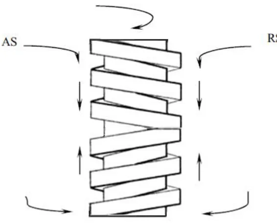
All three welding parameters can be seen visually in Figure 2.1.3. on the next page. This is shown

as a self-reacting pin tool type which will not include an anvil for the panels to rest on. This will

in turn make the pin tool pinch together at the set forge force instead of having an anvil with a

reaction force.

(18)

7

2.2 Frictional Heat

One of the more important factors of determining the effectiveness of the weld is to examine the

heat input from the pin tool to the work piece. It is estimated for a self-reacting weld, the generated

heat can be transferred to the work piece through conduction, lost to the ambient air through

convection and radiation, or transferred to the pin tool through conduction [7]. It is estimated that

at most 95% of the frictional heat can be transferred to the work piece [11]. The main methods of

varying the input heat is by changes in the weld parameters. The table below shows the relation

of the welding parameters with respect to the amount of frictional heat generated.

Table 2.2.1

Frictional Heat vs. Welding Parameter [12]

Welding

Parameter Decrease Parameter Increase Parameter

Forge Force Reduce Frictional Heat Increase Frictional Heat Tool RPM Reduce Frictional Heat Increase Frictional Heat Travel Speed Increase Frictional Heat Reduce Frictional Heat

As the work piece receives less heat the pin tool is then forced to apply more cold work to plasticize

the materials. This will allow the strength to increase along with the amount of proportional cold

work [11]. This is good in theory, but practically it requires much stronger pin tools, as they will

also bear stress of this increased cold work, resulting in potential fracturing of the pin tool. The

colder the weld will also yield a more brittle final product. The opposite of that in which a surplus

of heat is added to the work piece. This will result in a much more ductile weld.

The amount of heat will have an impact on the grain structure of the work piece. An increase in

the total heat supplied to the work piece will result in an enlarged grain structure. This is due to

(19)

8

defined as a process in which new strain-free grains are allowed to nucleate and replace previously

damaged grains [13].

2.3 Metallurgy

As the pin tool travels across the weld seam, the microstructure is modified. This allows sections

of the material to receive different heat treatments. These sections are divided up into the

following: Unaffected Material; Heat Affected Zone (HAZ); Thermomechanically affected zoned

(TMAZ); and, Weld Nugget [7]. Figure 2.3.1 shows a representation of the areas with respective

sizes. The amount of heat transferred to the work piece will also affect the total reach of the heat

affected zone.

Figure 2.3.1: Microstructure of a Friction Stir Weld [7]

The unaffected material will be the area of the panel that will still retain the original grain size and

orientation. The negligible amount of heat received in this area will not result in any

microstructure changes. If the panel has any specific grain size or orientation before the welding

(20)

9

The next area of interest is the Heat Affected Zone. The HAZ will have a grain structure that

undergoes recrystallization. The orientation of the grains will also remain constant and not change,

retaining the original orientation of the parent material. The grain size will also larger than the

nugget and TMAZ as it only undergoes static recrystallization and recovery.

The third area, the Thermomechanically Affected Zone, will experience more heat transfer than

the previous two zones, which this zone will start showing indications of the material flow. The

grain orientation will start following the material flow path instead of retaining the orientation of

the base material’s orientation. The grains in the TMAZ will experience similar conditions to hot

working on metal. As of what happens to the grains themselves, they will experience both dynamic

and static recrystallization and growth. This will cause the grain size to become even smaller, but

some larger grains can exist.

The last but most important zone is the weld Nugget. The nugget represents a highly turbulent

and complex zone with material flow, and varying stresses and different strains acting on the

material. The grain structure in this zone experiences full recrystallization which will result in the

most refined grain size that have an equiaxed orientation.

These four zones can then be identified on metallurgical macrograph pictures, in which an example

(21)

10

Figure 2.3.2: Zone Classification of a Friction Stir Weld [9]

2.4 Strength of Materials

The strength of the material is defined as the stress required to break the material under question.

The stress is the applied load on the subject material normalized by the cross-sectional area. This

can be equated below [14]:

𝝈 =

𝑷

𝑨 Eq. 2.4.1

The strain of the material is not the same as the stress, as it is a mathematically representation of

how far the atoms at any point in the solid are being pulled apart. This is normalized by the unit

length of the material in question. This can also be express mathematically as seen in Eq 2.4.2.

Engineering strains are often very small, and are often expressed in percentages instead of absolute

quantities [14].

𝛆 =

𝚫𝐋

𝑳 Eq. 2.4.2

These two units can be graph together to determine how a material reacted under various loading

(22)

11

future welds to be completed under similar conditions. A typical stress-strain curve is depicted in

Figure 2.4.1 and shows the various regions of interest.

Figure 2.4.1: Typical Stress-Strain Curve [15]

In the figure above, the graph on the left shows a typical stress-strain relation for a ductile material,

while the graph on the right side shows a graph for a typical brittle material. There are several

points of interest in the above stress-strain curves. The pl is the proportional limit which is the

maximum stress for which the linear relationship is valid. The el is marked as the elastic limit.

This is the region in which any applied deformations will yield back to the original condition and

not result in any permanent deformations. After the elastic region, any the recovery of the material

will be parallel to the straight line of the curve and will result in permanent deformation. This is

known as the plastic region. The yield point, y, is very close to the elastic point, and is often

considered where the plastic region begins. The ultimate strength is marked by u and is the

maximum stress a material can support without fracture. The last point of interest is the fracture

strength, labeled as f, in where the material actually fails. For ductile materials, the fracture

strength is actually less than the ultimate strength, this is because the material will neck down

(23)

cross-12

sectional area of the material will neck down, less applied load is required to pull the tensile

specimen at the designated rate [16] [17].

Engineering stress is one method of analyzing the stress-strain curve and for most purposes, is a

good approximation of the true stress. This is completed by calculating the stress per area using

the original unloaded tensile dimensions. When a material specimen undergoes loading, the

cross-sectional area will reduce under the applied load. The true stress will involve calculating the stress

with the continuous reductions in area. This is more instrument intensive as more data will have

to be collected. The stress and strain calculated in this report will be the engineering stress/strain.

Materials can be categorized into different groups based on the mechanical property: Ultimate

Strength, Yield Strength & Modulus of Elasticity. A strong material has a high ultimate strength,

whereas a weak material will have a low ultimate strength. A tough material will yield greatly

before fracturing, also known as a ductile material. A brittle material will yield very little before

fracture. When examining the Modulus of Elasticity, a hard material will have a high Modulus of

Elasticity versus a soft material, which will have a low modulus of material. All of these groups

are not inherently good or bad, but is dependent on the application of the material [16].

Combinations of these material types can be represented in Figure 2.5.2 by the below stress-strain

(24)

13

Figure 2.4.2: Stress-Strain Curves for Various Material Types [18]

The categories listed above can be visually seen from the above graphs. More ductile materials

are tough as opposed to brittle, while strong materials will have a much higher slope in the elastic

region than weak materials, which can as high as 45°.

Another means of determining how brittle versus ductile the material is to examine the fracture

type post tensile testing. Figure 2.4.2 shows the possible outcomes of a tensile test for different

(25)

14

Figure 2.4.2: Fracture Types for Tensile Testing [19]

The materials can then be classified as brittle materials (a), Semi-ductile materials (b), or ductile

materials (c). The semi-ductile materials are typical for metals, which is what should be expected

for the results of this study.

2.5 Hardness

Hardness is the measure of a material’s resistance to deformation by surface indentation or by

abrasion [13]. Hardness testing is a simple and inexpensive method for determining the

mechanical properties of a material. One method of measuring the hardness of the material is

through the Vickers Hardness test. This is completed through the means of a diamond shaped tool,

that is pressed against the surface of the material, creating an indentation. Hardness testing is

completed by having a diamond indented into the specimen. A smooth, firmly supported flat

surface is required, in which the load is normally applied for 30 seconds [20]. Typical loads for

these types of testing can range from 1 and 1000 grams [13]. The hardness of the material is then

related to the indention load, and the diagonal length of the diamond, which can be seen

(26)

15

method of hardness testing. To acquire these diagonal lengths, an optical microscopy must be

utilized.

𝑯𝑽

∝

𝑭

𝒅𝟐 Eq. 2.5.1

Figure 2.5.1: Typical Hardness Across Friction Stir Weld [7]

When examining typical mechanical properties of 2000 series aluminum alloys post friction stir

welding, it can be seen that the hardness per distance from the center follows a “W” pattern. This

means that the nugget is not the softest location on a friction stir weld. The TMAZ/HAZ

interference will have the lowest hardness, which is seen in the above figure at the sharp downturns

from the Parent material through the HAZ. This is due to the dissolution and growth of the

precipitates, which will in turn reduce the joint efficiency[22]. This is important to know as the

material will fail at the weakest point, which is not the nugget itself, in which it will often fail on

(27)

16

2.6 Tool Geometry

There are three different types of pin tool orientations that can be utilized for friction stir welding.

There are fixed pin, self-reacting pin, and adjustable pin. The welding done in this experiment

utilizes a self-reacting pin tool. A self-reacting pin tool is one in where no anvil is present. This

is practical as an anvil is not always available on welding certain structures. A self-reacting pin

tool consists of the normal shoulder and pin tool, but in addition to this, a bottom shoulder is

attached. The bottom shoulder is placed underneath the work piece in where the anvil would

normally be placed. This is completed by having the welding machine pull the bottom shoulder

up against the work piece while the top shoulder normally presses down against the work piece.

Both shoulders having the same pressing force against the workpiece as to not cause any vertical

deformation. This method will result in the total net force on the work piece to be zero [23].

An important aspect of pin tool selection to note would be that of the pin thread orientation. Most

standard pin tools have either a left-hand or right-hand thread orientation. These can be seen in

the two following figures.

(28)

17

The above figure is a pin tool with a right-hand thread orientation. This is because the threads

follow the right-hand grip orientation. It can be seen from the above that a weld that is completed

using a right-hand threaded pin tool, in the clockwise direction, the material will flow up towards

the top shoulder.

Figure 2.6.2: Material Flow of a Left-Hand Thread Pin Tool [24]

The above figure is a pin tool with a left-hand thread orientation. This is because the threads are

opposite to that of the right-hand grip orientation. It can be seen from the above that a weld that

is completed using a left-hand threaded pin tool, in the clockwise direction, the material will flow

down towards the bottom anvil, and in the case of self-reacting pin tool, the bottom shoulder.

The pin tool that was used for this experiment was a 3/8” pin tool with a Left-Hand Right-Hand

thread orientation. The total thread length was 7/16”, which provides plenty of clearance for the

.36” thickness of the workpiece. The welds were completed in a clockwise manner. This

orientation can be expressed visually in the Figure 2.7.3. It is noted that the shoulders are not

(29)

18

Figure 2.6.3: Left-Hand (Top) Right-Hand (Bottom) Threads Together

Examining the properties of material flow for each of the thread orientations, and then combining

them, it can be realized that the material for a Left-hand Right-hand pin tool used in a clockwise

manner will force the material to flow towards the center of the work piece.

It is also noted that having a pin tool with either a Left-Hand only thread orientation, or

Right-Hand only thread orientation that pushes the material in one direction will cause material to flow

towards one of the shoulders. This will cause the material to stick to either the top or bottom

shoulder, which will cause a lack of plasticized material for the remaining areas [25]. This will

cause an increase in the possibility of a weld to form porosity or lack-of bonding defects [26]. This

is because there will not be enough material for uniform mixing to occur in the weld which will

increase the probability of defects to form. In order to counter the material from flowing into one

of the shoulders in a self-reacting weld, a left-hand right-hand pin tool should be used in a manner

(30)

19

2.7 Design of Experiments

Design of Experiments (DOE) is a statistical approach of experimental design where several

variables will need to be altered over the course of the experiment. DOE was originally invented

by Ronald Fisher [27]. One of the main advantages of using a DOE approach as opposed to a

trial-and-error manner is that a range of process variables can be systematically tested in an organized

and much more efficient manner.

DOE consists of varying a set number of variables over a range of predetermined values. This

allows for the widest range and encompassing approach to an experiment but it can make the

experiment a lengthy process depending on the number of variables that are required. Design of

Experiments is defined by what is called the factorial. The number of variables and range can be

express in the equation below [28] [29].

Experiment Runs = 𝑳𝒆𝒗𝒆𝒍 𝒑𝒆𝒓 𝑽𝒂𝒓𝒊𝒂𝒃𝒍𝒆𝒔𝑵𝒖𝒎𝒃𝒆𝒓 𝒐𝒇 𝑽𝒂𝒓𝒊𝒂𝒃𝒍𝒆𝒔 _{Eq. 2.7.1}

Each variable will have different individual values, or levels, that it will be cycled through. This

is dependent on the process variables and the range that they will be varied through. Looking at

how friction stir welding has three primary process variables, forge force, travel speed and spindle

RPM, it can be deduced that a full three factorial DOE should be used for an experiment of this

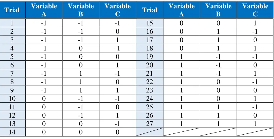
magnitude. An example of a three-factorial approach in where an experiment would have three

variables with three different levels per variable is tabulated in Table 2.7.1. This would result in

(31)

20

Table 2.7.1

3

Factorial Approach

Trial Variable A

Variable B

Variable

C Trial

Variable A Variable B Variable C

1 -1 -1 -1 15 0 0 1

2 -1 -1 0 16 0 1 -1

3 -1 -1 1 17 0 1 0

4 -1 0 -1 18 0 1 1

5 -1 0 0 19 1 -1 -1

6 -1 0 1 20 1 -1 0

7 -1 1 -1 21 1 -1 1

8 -1 1 0 22 1 0 -1

9 -1 1 1 23 1 0 0

10 0 -1 -1 24 1 0 1

11 0 -1 0 25 1 1 -1

12 0 -1 1 26 1 1 0

13 0 0 -1 27 1 1 1

14 0 0 0

Due to the lengthy process required by a full three factorial approach and the large number of

weldable panels required, a modified three factorial approach was used, in where one variable of

the three variables was held constant, the second variable only had two process levels and the third

was fully varied through three separate levels. An example of this can be seen below in Table

2.7.2 in where this would be deemed a 11 21 31 Factorial Approach. Using Eq 2.7.1 to multiply

(32)

21

Table 2.7.2

1

₂

1

₃

1

_{Factorial Approach}

Trial Variable A Variable B Variable C

1 1 -1 -1

2 1 -1 0

3 1 -1 1

4 1 0 -1

5 1 0 0

6 1 0 1

Once the experiments are run, the finished data can be input into a linear regression analysis. A

regression analysis is a statistical technique for investigation and modeling the relationship

between variables and explain any possible relationships between them [30]. The goal of the linear

regression model is to determine the relationship between the dependent variables and the

independent variables expressed in the Eq 2.7.2

Eq. 2.7.2

This equation can be used for several variables, but for this experiment a two-variable case will be

utilized. For the two-variable case, in where the travel speed and Force/RPM will be analyzed,

the slopes of each dependent variable can be solved for in the below equations:

Eq. 2.7.3

The above two equations require further manipulation of the data by solving for the product of

(33)

22

Eq. 2.7.4

The only remaining variable which is needed to model the regression line will be the intercept,

which can be solved by inputting all known quantities into Eq. 2.7.2 and solving for the last

remaining variable [31]. From there the values of the actual dependent variables versus the

predicted dependent variable can be plotted together to determine the accuracy of the linear

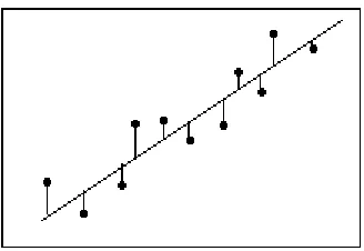
regression line. When these values are plotted together, the residual will become apparent. The

residual is known as the difference between the predicted value and actual value. Looking at

Figure 2.7.1, the actual value would be the black dots and the predicted value is the straight line

between them calculated using the regression model. The vertical lines connecting the two objects

is the residual amount [32].

Figure 2.7.1: Graphical Representation of Residual

The accuracy of the regression line can be expressed using the R2 value of the computed data. The

R2 value is a number that is always ranges from 0 to 1, or 0% to 100%. The R2 is also a good

(34)

23

then be calculated based on the following equation or computationally through readily available

programs like Microsoft Excel [33].

𝑹

𝟐

= 𝟏 −

𝑺𝑺𝒓𝒆𝒔

𝑺𝑺_𝒕𝒐𝒕 Eq. 2.7.5

Once an actual value for R2_{is defined, the fit of the linear regression model can then be determined.}

A low value indicates that the linear regression model is not a good predictor of the data points,

while a number closer to 1 indicates that it will. Figure 2.7.2 below shows a linear regression

model for a set of data points with an R2 value closer to 1. This is because the linear regression

model does not miss many of the data points by a significant amount and is a good predictive

model for a trend.

Figure 2.7.2: Example Linear Regression Model with High R2_{Value [34]}

Once the final values of the regression model the error can be quantified by the Eq. 2.7.6 labeled

below.

𝑬𝒓𝒓𝒐𝒓 (%) =

|𝑴𝒆𝒂𝒔𝒖𝒓𝒆𝒅 𝑽𝒂𝒍𝒖𝒆−𝑷𝒓𝒆𝒅𝒊𝒄𝒕𝒆𝒅 𝑽𝒂𝒍𝒖𝒆|

(35)

24

Chapter 3: Research Conducted

3.1 Welding & Machining

The researched that was completed consisted of determining of weld parameters, welding the test

panels together, tensile testing, macrograph analysis and micro-hardness testing.

The first step in the research was to determine the welding parameters. It was decided to vary the

travel speed as a pin tool previously broke when a forge force of 4000 lbf was applied. With

respect to the integrity of the equipment, a more conservative weld scheme was selected due to

limited supplies. The final weld parameters were chosen based off of the previous research

conducted by the undergraduate Friction Stir Welding class final projects. The original scope of

their research project did not include variable insensitivity.

Figure 3.1.1: Previous Nominal Dataset [35]

Figure 3.1.1. above is important as it shows the forge force variable insensitivity of the previous

nominal dataset. The importance of this graph shows that a certain combination of welding

parameters will have mechanical properties independent of forge force. The bow-tie affect that is

0 10 20 30 40 50 60

12 13 14 15 16 17 18 19 20 21 22

(36)

25

desired is clearly on display and it is one of the goals of this manuscript to recreate this affect by

varying different welding parameters. This provided a prediction to create welding parameters

that can be seen in Table 3.1.1 that would result in the desired output instead of trial and error.

This dataset varies the forge force similar to the original experiment discussed in Chapter 1.

It can be seen that a Rotation per Inch (RPI) range of 14 to 21 can be used to recreate the desired

bow-tie effect. With this knowledge in hand, similar process variables were developed based off

of this fact. For this experiment, the RPI was chosen to be in the range of 13 to 25 to encompass

a larger range as it was noted that the bow-tie effect would diminish under lower travel speeds, but

this data was inferred from a smaller data range. A middle point between the two extremes was

selected to see if the insensitive point could be recreated. The complete results in this experiment

will be displayed with respect to Force/RPM instead of RPM/IPM since the travel speed was varied

instead of the forge force.

Table 3.1.1

Welding Parameters Used in the Experiment

Weld Forge Force IPM RPM Force/RPM

W1 2400 13 180 13.33

W2 2400 13 215 11.16

W3 2400 13 275 8.72

W4 2400 11 180 13.33

W5 2400 11 215 11.16

W6 2400 11 275 8.72

The advancing side was Aluminum 2195 with a gauge thickness of .35”, while the retreating side

was Aluminum 2219 with a thickness of .36”. As to why the weld panels did not possess the same

thickness, the weld panels were chosen amongst readily available materials. Each weld panel is

24” long, with a width of 4”. There was a total of 12 weld panels used in the course of this

(37)

26

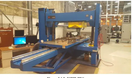
Each weld was completed at NASA Michoud Assembly Facility using the ISTIR PDS, seen in

Figure 3.1.2. This equipment is owned by the National Center of Advanced Manufacturing

(NCAM), and is able to be used by college students of state owned Louisiana colleges. This

machine possesses customizable tool heads, allowing it to also be the same machine that the

specimens were fly cut on.

Figure 3.1.2: ISTIR PDS

Each weld had a start hole drilled to allow for the self-reacting pin tool to be put into place. This

means that the pin tool does not plunge into the material like that of a fixed pin or retractable pin.

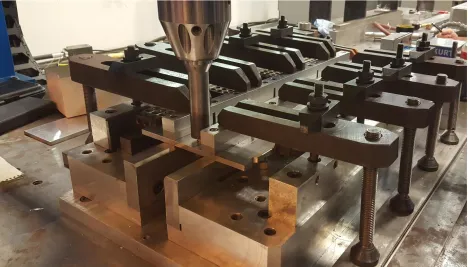
The welds were then clamped down, as shown below, as to prevent any displacement of the plate

itself. This was completed using side 8 side clamps, 4 per side, resting along a clamp bars. This

is to distribute the clamp force evenly along the length of the weld, and to prevent each side clamp

(38)

27

would cause localized bending stresses along the weld panel and this could compromise the

integrity of the weld.

Figure 3.1.3: Typical Set-up for each Weld

(39)

28

The welds are completed by the ISTIR PDS with a preset program. These programs tell the

machine where to start and finish the weld, how fast each part spins or moves, and how long of a

warm up period is required to create a good weld.

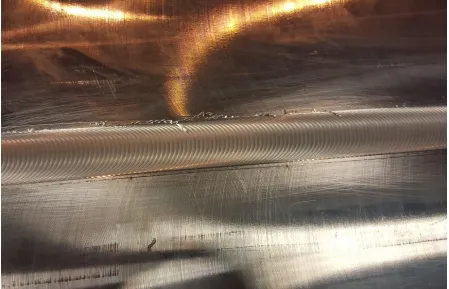
Once the welds are completed using the above methods, they were then removed from the

clamping apparatus and then taken to have the scroll lines removed. These scroll lines need to be

removed as to prevent stress concentrations during tensile testing. They were removed using a

medium grit 3MTM Scotch-BriteTM RolocTM Surface Conditioning Disc. Both sides of the welded

panel had any scroll lines removed down to a smooth surface, but not so much removed as to where

the disc would dig into weld causing unwanted low points. The pin tool and shoulder were then

subsequently cooled between each weld to prevent residual heat from being transferred to the next

weld.

(40)

29

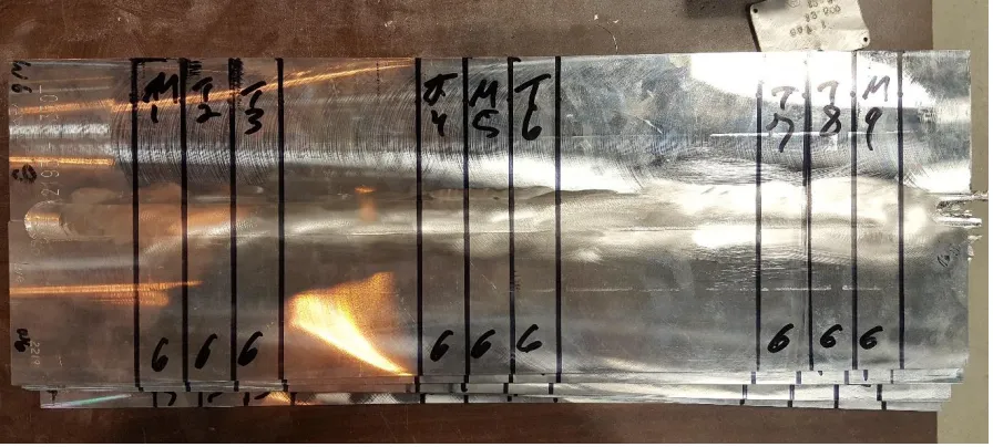
After the scroll lines were removed, the welded panel was then separated into nine individual

specimens by use of a band saw. Six were to be used as tensile specimens, while the remaining

three were to be used for macrographs and hardness testing. The locations of each of the tensiles

and macros in this experiment are labelled in Figure 3.1.6. Each cut is 1.2” wide with

pre-measured spacing in between each specimen resulting in a total of nine specimens. This was

completed for each weld resulting in a total of 36 tensile specimens and 18 macrograph/hardness

specimens. Due to the inaccuracy of the band saw and human error present along the seams of the

cut, the specimens then had to be further machined down to a uniform width across each specimen.

Figure 3.1.6: Tensile and Macrograph Locations

As mentioned before, the ISTIR PDS has interchangeable tools that allowed for the fly cutting to

occur. Figure 3.1.7 dictates an image of the process, in where the fly cutter was spun at a preset

speed of 1300 RPM, in where the tool was then passed across the specimens removing at a

maximum of .020” of the thickness each time. This process was repeated until the side being

worked on had a smooth finish. This was then repeated on the other side of the specimens until a

smooth side was present. This resulted in the specimens for that particular weld to have a uniform

(41)

30

to ensure that the tensile specimens for one weld all had the same dimensions. It was noted by

clamping the specimens together that any scribe marks that were placed on the sides of a specimen

were imprinted on the adjacent specimen. These had to removed post fly-cutting by use of the

Scotch Brite pads.

Figure 3.1.7: Machining Tensiles to Uniform Width

3.2 Tensile Testing

Once the tensile specimens were machined down to uniform widths, they then underwent tensile

testing. The gauge length of 4” was used for the tensile testing. This was to have a wider area to

allow for necking. If a shorter gauge length was used, this would allow the possibility of the

specimen necking outside of the predetermined area. The exact measurement that was used for

the gauge length was 3.94”.

The tensile tests were completed on an MTS 810 material testing machine. This is completed by

inputting a feed rate and then the machine will determine and output the force necessary to keep a

(42)

31

constant feed rate will lower as the cross-sectional area reduces. This will explain why the fracture

stress is lower than the ultimate stress for more ductile materials.

Figure 3.2.1 shows a tensile test post fracture. The larger of the two load cells was used (55 kip

vs 22 kip). The 55 kip load cell was used because previously the 22 kip load cell was almost at

full capacity at breaking .320” thick specimens. The specimens in this experiment were larger,

and a more conservative approach was taken with regards to maximum force output.

The MTS 810 outputs all data points recorded during the testing period on an excel spreadsheet.

Each tensile has its own unique spreadsheet with the data recorded. The data points collected are

the displacement, the force and if an extensometer is utilized, the deformation can also be recorded.

The elongation was then calculated by the displacement recorded from determining the spring

constant of the machine itself.

(43)

32

After each tensile was broken, the specimen was then removed and the final elongation was

recorded. This was completed by pressing the specimen back together and recording the distance

between the grip marks on the specimen. This number was then used with the original 3.94” gauge

length to calculate the final elongation of the specimen.

3.3 Polishing & Macrographs

When examining Figure 3.1.6, the specimens that are labelled M1, M5, and M9 are to be used for

polishing and further macrograph analysis. For each weld, three areas were collected and

analyzed. This was the beginning of the weld, the center and the end of the weld. These three

zones will show the effects the weld has on the microstructure as it progresses through. This

resulted in a total of 18 separate macrographs which will then be later hardness tested.

The first part of process was to cut the tensile so that only 1.2” would be present centered through

the weld seam so that it may be mounted. This would allow all heat affected zones to be present

as a Macrograph and including some parent material for comparison. Once this was done, the

(44)

33

Figure 3.3.1: CitoPress [37]

This was done by first applying anti-stick cream to the inner area and then placing the specimen

inside. 50 mL of MultiFast red was then placed on top to cover the specimen. The sample was

then subjected to high temperature and pressure cycle to solidify the resin. Each sample was run

at 200 bars for a 2-minute heating period at 180 °C and then cooled for 1.5 minutes.

Once all specimens were fully mounted, they were then placed in a TegraMin to have

semi-automated specimen preparation completed, seen in Figure 3.3.2. The grinding and polishing of

(45)

34

Figure 3.3.2: TegraMin [38]

This first step in this process is to rough grind the specimen. This was completed by mounting the

specimens on a rotating head that spins at 150 RPM at 25N, with a 220-grit abrasive pad rotating

in the opposite direction at 300 RPM. This step was run for a total of 1:10 minutes. In all

subsequent steps the specimen holder is run at these conditions, with varying input forces, and the

pad is co-rotated.

The second step was to fine grind the specimen using the same setpoints as step 1, but instead use

a 500-grit abrasive pad. This step was run for a total of 4 minutes.

The third step utilized a Largo Disc, which is a composite disc for fine grinding, that was rotated

at 150 RPM and had a 20 N force applied for a 5-minute duration.

The fourth step utilized a Mol Disc, which is a woven wool disc for fine grinding, that was rotated

at 150 RPM and had a 20 N force applied for a 6-minute duration with the specimen rotating at

(46)

35

The fifth step is the first of the polishing steps and uses a Mol cloth polishing disc and run under

the same conditions as Step 4.

The sixth step, fine polishing, has a Dur polishing cloth being used, which has typical uses for fine

grinding of metals. The force was lowered to 15 N and the duration was increased to 7 minutes.

The seventh step, extra fine polishing, utilized a Plus polishing cloth disc, where the force was

lowered even more to 10 N and the duration was further increased to 10 minutes.

The eighth step utilized a Struers Chem polishing pad with agglomerated alumina lubricant for a

twenty-minute duration at 10 Newtons force while the polishing pad was rotated at 80RPM

co-directionally with the specimen holder as it rotated 150 RPM. Lastly, oxidative polishing utilized

a separate Chem pad and etchant which entailed concentrated hydrogen peroxide to enhance

etching properties. The oxidative polishing step lasted a 30:00-minute duration at 10 Newtons

force while the chem pad was rotated 70 RPM counter rotationally as the specimen holder, which

was also rotated at 150 RPM.1

Once completed the polished and mounted specimens had a 9% hydrogen peroxide solution

applied via the Chem disc used in step 8 for 20 minutes, and after this final step, macrographs were

then taken of each sample.

3.4 Hardness Testing

The specimens that were ground and polished for macrographs then had micro-hardness testing

completed. Micro-hardness is completed by indenting a diamond shaped indenter with a constant

size and force into the surface of the material. The test was performed using the Vickers pyramidal

1_{The process for grinding and polishing the specimens was developed by the University of New Orleans}

(47)

36

indenter at a force of 50 kg. Hardness testing requires bringing the specimen to a mirror-fine

polish. The specimen surface must be completely smooth and free of deformities as any

deformities would result in inaccurate readings. The hardness tester used for this experiment is

the Shimadzu hardness tester.

(48)

37

Chapter 4: Results

The first process in examining the welds will be to look at the physical aspects of the welds

themselves post welding, post tensile breaking and macrographs. Figure 4.1 shows the tensile

specimens of Weld 1 after they were broken. The advancing side is on the left, while the retreating

side is on the right. The tensiles in the figure are laid in an increasing order with Tensile #2 at the

top, and Tensile #8 at the bottom. Looking at the cracks, the beginning of the weld was more

likely to break on the advancing side, but along the length of the weld, the crack size and location

begins to change. The cracks become more jagged and begin to break along the center of the weld

nugget instead of the TMAZ. This could mean that a proper material mixing was not achieved

along the weld seam over the length of the weld. Examining the fracture break direction, tensiles

7 and 8 are much different than the previous four tensiles. The break type is more in line with a

brittle material as opposed to a ductile material due to the rough jagged edges. It can also be seen

that on tensile 7, there is a hairline crack normal to the applied force during the testing.

(49)

38

Figure 4.2 shows the tensile specimens of Weld 2 after they were broken. The advancing side is

on the left, while the retreating side is on the right. The tensiles in the figure are laid in an

increasing order with Tensile #2 at the top, and Tensile #8 at the bottom. Weld 2 shows an increase

in consistent ductility over Weld 1. This can be seen as fractures are cleaner and slight necking is

noticed along the edges. The tensiles are not jagged which is normally seen on brittle material

fractures. The tensiles also consistently broke near the retreating side of the TMAZ. The fracture

type throughout the six tensiles was largely consistent with very little variance in fracture angle

and type. Each tensile broke at a roughly 45° angle and did not show any signs of rough jagged

edges.

Figure 4.2: Weld #2 Post Tensile Break

(50)

39

a decrease in ductility from weld 2 as the breaks are no longer a ta 45° plane. The fracture was

found to be close to the TMAZ on the advancing side of the weld which is counterintuitive as the

metal on the advancing side has higher mechanical properties, making it the stronger side.

increasing order with Tensile #2 at the top, and Tensile #8 at the bottom. Weld 4 had similar input

parameters as Weld 1 and when comparing the two, they are similar in terms of how the tensiles

are experiencing brittle fractures. The last tensile does experience a slight change in the fracture

type as it becomes more brittle then the previous 5 tensiles. This indicates, like weld 2, that

improper mixing must be occurring at the later stages of the weld causing a drop in ductility. The

tensiles also had a tendency to break towards the advancing side along what appears to be the

(51)

40

increasing order with Tensile #2 at the top, and Tensile #8 at the bottom. When comparing to the

previous welds, the input parameters are closest to that of weld 2. The fractures do indicate a

decrease in ductility as the lack of a noticeable necking region along with the more jagged edges.

The fractures were close to the advancing side along the weld nugget which is opposite to that of

(52)

41

increasing order with Tensile #2 at the top, and Tensile #8 at the bottom. When comparing these

tensiles post break to Weld 3, which had similar welding parameters, a drop-in ductility can be

noticed from the crack propagation and lack of necking on the edges. The fractures were also

(53)

42

It is noted that Weld 3 and 6 both experience a weld defect known as lack of consolidation. This

can be seen in the Figure 4.7 below, with a red circle identifying the area of concern. There is a

visual indication that the weld was not properly consolidated under these input parameters. The

common similarity between Weld 3 and 6 is that both of them are using the highest RPM setting

at 275. The welds with lower rotations per inch did not show signs of lack of consolidation from

external examination.

(54)

43

The results of all testing are organized by the mechanical properties: elongation, the yield strength

and the ultimate strength; the macrograph analysis; and the hardness testing. The results will be

compared to the original abstract of this experiment in where it will be determined if certain

properties will be insensitive to variations of welding parameters and provide consistent results

(55)

44

Table 4.1

Elongation for Tensiles

Speed = 13 IPM

Force = 2400 lbf, Rotation = 180 RPM Force = 2400 lbf, Rotation = 215 RPM Force = 2400 lbf, Rotation = 275 RPM

Tensile Final Length (inches) ΔL (inches) Elongation

(%) Tensile

Final Length (inches) ΔL (inches) Elongation

(%) Tensile

Final Length (inches) ΔL (inches) Elongation (%)

W1T2 4.252 0.312 7.92 W2T2 4.271 0.331 8.40 W3T2 4.188 0.248 6.29

W1T3 4.215 0.275 6.98 W2T3 4.2155 0.2755 6.99 W3T3 4.254 0.314 7.97

W1T4 4.19 0.25 6.35 W2T4 4.2385 0.2985 7.58 W3T4 4.129 0.189 4.80

W1T6 4.271 0.331 8.40 W2T6 4.425 0.485 12.31 W3T6 4.182 0.242 6.14

W1T7 4.159 0.219 5.56 W2T7 4.219 0.279 7.08 W3T7 4.152 0.212 5.38

W1T8 4.192 0.252 6.40 W2T8 4.257 0.317 8.05 W3T8 4.2225 0.2825 7.17

Speed = 11 IPM

Tensile Final Length (inches) ΔL (inches) Elongation

(%) Tensile

Final Length (inches) ΔL (inches) Elongation

(%) Tensile

Final Length (inches) ΔL (inches) Elongation (%)

W4T2 4.1905 0.2505 6.36 W5T2 4.139 0.199 5.05 W6T2 4.1705 0.2305 5.85

W4T3 4.133 0.193 4.90 W5T3 4.1865 0.2465 6.26 W6T3 4.0765 0.1365 3.46

W4T4 4.1895 0.2495 6.33 W5T4 4.2865 0.3465 8.79 W6T4 4.1575 0.2175 5.52

W4T6 4.144 0.204 5.18 W5T6 4.0855 0.1455 3.69 W6T6 4.165 0.225 5.71

W4T7 4.139 0.199 5.05 W5T7 4.19 0.25 6.35 W6T7 4.0755 0.1355 3.44

(56)

45

Table 4.2

Yield Stress for Tensiles

Speed = 13 IPM

Tensile 𝜎_𝑦 (ksi) Tensile 𝜎_𝑦 (ksi) Tensile 𝜎_𝑦 (ksi)

W1T2 31.88 W2T2 33.25 W3T2 33.383

W1T3 32.09 W2T3 32.58 W3T3 33.22

W1T4 31.9 W2T4 32.45 W3T4 33.38

W1T6 32.34 W2T6 32.42 W3T6 33.58

W1T7 19.93 W2T7 33.43 W3T7 32.67

W1T8 36.29 W2T8 33.67 W3T8 32.64

Speed = 11 IPM

Tensile 𝜎_𝑦 (ksi) Tensile 𝜎_𝑦 (ksi) Tensile 𝜎_𝑦 (ksi)

W4T2 31.86 W5T2 31.74 W6T2 29.63

W4T3 31.44 W5T3 31.57 W6T3 28.43

W4T4 31.87 W5T4 31.04 W6T4 28.84

W4T6 31.78 W5T6 32.33 W6T6 30.40

W4T7 32.07 W5T7 31.95 W6T7 29.53

(57)

46

Table 4.3

Ultimate Strength for Tensiles

Speed = 13 IPM

Tensile Maximum

Force (lbf)

Area (in2)

𝜎𝑢

(ksi) Tensile

Maximum Force (lbf)

Area (in2)

𝜎𝑢

(ksi) Tensile

Maximum Force (lbf) Area (in2) 𝜎𝑢 (ksi)

W1T2 17,923 0.36 49.79 W2T2 16,540 0.32 50.99 W3T2 17,731 0.36 49.25

W1T3 18,092 0.36 50.26 W2T3 15,998 0.32 49.43 W3T3 18,115 0.36 50.32

W1T4 18,076 0.36 50.21 W2T4 16,156 0.32 49.92 W3T4 16,933 0.36 47.04

W1T6 18,060 0.36 50.17 W2T6 16,072 0.32 49.66 W3T6 17,556 0.36 48.77

W1T7 9,610 0.36 26.69 W2T7 16,042 0.32 50.64 W3T7 17,123 0.36 47.57

W1T8 14,474 0.31 47.01 W2T8 16,102 0.32 50.83 W3T8 16,867 0.36 46.85

Speed = 11 IPM

Tensile Maximum

Force (lbf)

Area (in2)

𝜎_𝑢

(ksi) Tensile

Maximum Force (lbf)

Area (in2)

𝜎_𝑢

(ksi) Tensile

Maximum Force (lbf) Area (in2) 𝜎_𝑢 (ksi)

W4T2 13,746 0.36 38.18 W5T2 14,064 0.36 38.87 W6T2 10,992 0.34 32.14

W4T3 14,338 0.36 39.83 W5T3 13,260 0.37 35.94 W6T3 10,960 0.34 32.05

W4T4 14,483 0.36 40.64 W5T4 14,523 0.38 38.42 W6T4 11,116 0.34 32.50

W4T6 13,719 0.36 38.11 W5T6 13,524 0.35 38.53 W6T6 11,543 0.34 34.11

W4T7 14,342 0.36 40.24 W5T7 12,836 0.35 36.57 W6T7 11,187 0.34 32.71

(58)

47

All macrographs can be found in Chapter 7. Upon examining the macrographs, it is noted that the

shape of the weld 2195 portion of the weld nugget is changed as the RPM increases. The lower

RPM welds have the nugget looking more like a flame as it is not as compact and waviness is

found throughout. As the RPM increases, the welds begin to consolidate more in the middle and

have a thinner overall layer of material across the latitudinal centerline.

Looking at the shape of the macros it can be deemed that the welding parameters have an effect

on the overall shape of the weld nugget. The higher RPM welds have less waviness overall and a

more concise 2195 material profile. This is because the spindle is able to mix the material more

and cause a more concise weld. When comparing the same RPM values the travel speed also has

an effect on this, as the slower travel speed has less waviness. This is because the spindle is

allowed more contact with a particular location on the weld itself. The voids tend to be more

apparent on the lower RPM welds, also because the spindle is not able to uniformly mix the

material together and instead is leaving voids as it is passing through the area.

Looking at the size of the 2195 material length, or nose, in the weld nugget, the center of the welds,

or M5, possesses the larger weld nuggets when compared to the M1 & M9, the beginning and end

of the weld respectively. This was consistent across all welds, as the beginning of the weld and

end of the weld were normally thinner. Normally in friction stir welding the start point and end

point are completed on raised lips and these cut off post machining to avoid this type of

irregularities in the microstructure.

The nose length for most of the welds had a trend where it increased over the length of the weld,

where the alternative would be the center of the weld had a decrease in nose length, and the outer

(59)

48

average. This could be due to the fact that the higher RPM would produce more heat, allowing

the material to be extruded and flow much more easily.

The length of the nose has an effect on the material properties, with W5M9 being a great example

as it has a very long nose, and the properties are trending downward as they approach this sample

location. When comparing the required forces to break each tensile, as the material had a longer

nose on that particular point of the weld, a lower force was required to break the tensile specimen.

It is expected that this nose length would also be determined by the forge force as a higher forge

force will allow the material to extrude further, but cannot not be confirmed in this study, as all

welds were completed at the same forge force value.

Voids were present in the weld and it can be seen in the macrographs. They appear as white spots

as the silicon used in the grinding/polishing process was lodged into them and filled the void. The

silicon was unable to be removed, but it did make finding the voids much easier. The voids are

present more in the higher travel speed welds when compared to the lower travel speed welds.

Figure 4.9 shows the locations of these voids on a particular weld. The voids are prevalent on both

(60)

49

Figure 4.8: Voids in Weld

As noted early in this paper, a lack of consolidation defect was noted on the surface of welds 3 &

6. It appears that this defect is closer to the advancing side. This can be also seen in the

macrographs, displayed in Figure 4.10. On the advancing side, it is seen where the discoloration

(61)

50

Figure 4.9: Lack of Consolidation

The hardness testing results can be seen tabulated below in Table 4.5 which shows the total range

of the hardness values on each side of the weld, while the remaining hardness data plots can be

found in Chapter 7. These values are taken from the HAZ to the point of the 2195/2219 material

Analysis of Variable Insensitive Friction Stir Welding Parameters

ScholarWorks@UNO

ScholarWorks@UNO

Analysis of Variable Insensitive Friction Stir Welding Parameters

Analysis of Variable Insensitive Friction Stir Welding Parameters

Analysis of Variable Insensitive Friction Stir Welding

Acknowledgement

Table of Contents

Nomenclature

List of Figures

List of Tables

Abstract

Chapter 1: Introduction

Table 1.1

Mechanical Properties for Aluminum Alloys

Chapter 2: Literature Review

2.1 Friction Stir Welding

2.2 Frictional Heat

2.3 Metallurgy

2.4 Strength of Materials

𝝈 =

𝛆 =

2.5 Hardness

𝑯𝑽

∝

2.6 Tool Geometry

2.7 Design of Experiments

Table 2.7.1

3

Factorial Approach

Table 2.7.2

1

2

3

Factorial Approach

𝑹

= 𝟏 −

𝑬𝒓𝒓𝒐𝒓 (%) =

Chapter 3: Research Conducted

3.1 Welding & Machining

Table 3.1.1

Welding Parameters Used in the Experiment

3.2 Tensile Testing

3.3 Polishing & Macrographs

3.4 Hardness Testing

Chapter 4: Results

Table 4.1

Elongation for Tensiles

Table 4.2

Yield Stress for Tensiles

Table 4.3

Ultimate Strength for Tensiles

₂

₃

_{Factorial Approach}