Investigation of Surface Displacements Induced in Loaded Cross-Ply Composite Laminates with Microcracking

(1)

ScholarWorks@UNO

University of New Orleans Theses and

Dissertations Dissertations and Theses

5-21-2004

Investigation of Surface Displacements Induced in Loaded

Cross-Ply Composite Laminates with Microcracking

Ply Composite Laminates with Microcracking

Balakishore Rayasam

University of New Orleans

Follow this and additional works at: https://scholarworks.uno.edu/td

Recommended Citation Recommended Citation

Rayasam, Balakishore, "Investigation of Surface Displacements Induced in Loaded Cross-Ply Composite Laminates with Microcracking" (2004). University of New Orleans Theses and Dissertations. 94.

https://scholarworks.uno.edu/td/94

This Thesis is protected by copyright and/or related rights. It has been brought to you by ScholarWorks@UNO with permission from the rights-holder(s). You are free to use this Thesis in any way that is permitted by the copyright and related rights legislation that applies to your use. For other uses you need to obtain permission from the rights-holder(s) directly, unless additional rights are indicated by a Creative Commons license in the record and/or on the work itself.

(2)

INVESTIGATION O

F

SURFACE DISPLACEMENTS INDUCED IN

LOADED CROSS-PLY COMPOSITE LAMINATES WITH

MICROCRACKING

A Thesis

Submitted to the Graduate Faculty of the University of New Orleans in partial fulfillment of the requirements for the degree of

Masters of Science in

The Department of Mechanical Engineering

by

Balakishore V Rayasam B.Tech, Nagarjuna University, 2000

(3)

ii

Acknowledgements

I would like to thank Dr. Melody Verges for introducing me to the field of microcracking

in composites and for all her continuous and patient support. This study was carried out

with her vision and ideas.

I would also like to thank Dr. Paul Herrington for clarifying my doubts on ANSYS.

I wish to thank Dr. Paul J Schilling for attending the defense and his graduate students

Arun Kumar and Bhanu for their guidance in documentation.

I wish to thank to Krishna Kumar Kasturi and Rajiv Mididoddi for their help on

drawings.

(4)

iii

List of Figures

Figure 1.1 Schematic showing the surface displacement Parameters 3 characterizing penny-shaped cracks in homogeneous materials

Figure 2.1 Schematic of microcrack development and progression 9 in 900 ply upon application of transverse loading

Figure 2.3 Schematic for ultrasonic polar back scattering technique 16

Figure 2.4 Schematic for showing planes of the transducer and crack 16

Figure 3.1 Tensile sub stage used to load the specimen 19

Figure 3.2 Schematic of a shearography set-up 23

Figure 3.3 Schematic for creation of lateral sheared images 24

Figure 3.4 Schematic showing images being recombined 25

Figure 4.1 Schematic of [0/90]s composite laminate with 28

microcrack in 90°plies

Figure 4.2 Schematic of 8-noded solid 45 brick element 30

Figure 4.3 Schematic of 20-noded solid 95 brick element 30

(7)

vi

Figure 4.5 Isotropic view of the quarter model 32

Figure 4.6 Boundary conditions around the vicinity of the microcrack 33

Figure 4.7 Force (depicted by arrows) on the quarter model 35 of the 0/90/90/0 laminate

Figure 4.8 Convergence of out-of-plane displacements along the profile 36 plane of the quarter model for the [0/90/90/0] IM7/977-2

laminate loaded to 1000 MPa

Figure 5.1(a) Out-of plane contours on the top surface of a [0/90/90/0] 37 laminate with a microcrack extending through both 90 plies

and a transverse loading of 1000 MPa. In this picture a 2mm section in length is shown with the microcrack located in the center. The width of the crack is taken to be 5mm. Each contour represents an interval of 100 nanometers.

Figure 5.1(b) Out-of plane contours on the top surface of a [0/90/90/0] 38 laminate with a microcrack extending through both 90 plies

and a transverse loading of 1000 MPa. In this picture a 2mm section in length is shown with the microcrack located in the center. The width of the crack is taken to be 10mm. Each contour represents an interval of 100 nanometers.

Figure 5.2 Uy nodal solution at the xy mid-plane for a section length 39 of x = -1 mm to 1 mm for a [0/90/90/0] laminate with a

microcrack extending through the 90 plies and a transverse loading of 1000 MPa. In this graph each contour represents 100 nanometers.

Figure 5.3(a) Schematic defining the surface parameters 42

Figure 5.3(b) Schematic defining the laminate parameters 42

Figure 5.4(a) Mesh of the [0/0/90]slaminate 43

(8)

vii

Figure 5.5 Uy displacements along profile plane for four cross-ply 49 transversely loaded to 1000 MPa. For each case, the

microcrack length is the increasing. The depth of the crack below the surface is kept constant. (The far-field Uy displacements have been subtracted out of the profile.)

Figure 5.6 Uy displacements along profile plane for four cross-ply 50 transversely loaded to 1000 MPa. For each case, the

microcrack length is the same. The depth of the crack below the surface is varied. (The far-field Uy displacements have been subtracted out of the profile.)

Figure 5.7 Uy displacements along profile plane for cross-ply laminates 51 totaling a laminate thickness of 6t transversely loaded to

1000 MPa. (The far-field Uy displacements have been subtracted out of the profile.)

Figure 5.8 Uy displacements along profile plane for cross-ply laminates 52 totaling a laminate thickness of 8t transversely loaded to

1000 MPa. (The far-field Uy displacements have been subtracted out of the profile.)

Figure 5.9 Graph showing variation of maximum peak value for a load 53 of 1000MPa. Case A represents four laminates with crack

tips the same distance below the surface. The microcrack length varies according to ply thickness as shown. Case B represents four laminates having the same size microcrack. The depth of the crack tip below the surface varies with ply thickness as shown.

Figure 5.10 Graph showing variation of difference between peak and 53 minimal values. Case A represents four laminates with crack

(9)

viii

Figure 5.11 Comparison of Uy displacement for [0/90] s and [0/0/90/90] s 54

laminates. (The far-field Uy displacements have been subtracted out of the profile.)

Figure 5.12(a) Uy displacement pattern for a section length of x = -1 mm 56 to 1 mm for a [0/90/90/0] laminate with a microcrack extending through the 90 plies and a transverse loading of 1000 MPa.

Figure 5.12(b) Uy displacement pattern for a section length of x = -1 mm 57 to 1 mm for a [0/90/90/90/90/0] laminate with a microcrack

extending through the 90 plies and a transverse loading of 1000 MPa.

Figure 5.12(c) Uy displacement pattern for a section length of x = -1 mm 57 to 1 mm for a [0/0/90/90/0/0] laminate with a microcrack

extending through the 90 plies and a transverse loading of 1000 MPa.

(10)

ix

LIST OF TABLES

Table I. Surface Parameter Values for different Ply Orientations 44

and Loadings.

Table II. Surface Parameter Values for different Ply Orientations 58 where dct = t and loading = 1000 MPa

Table III Surface Parameter Values for different Ply Orientations 58 where a = t and loading = 1000 MPa

Table IV Surface Parameter Values for different Ply Orientations 59 where d = 4t and loading = 1000 MPa

(11)

x

Abstract

This work is aimed at investigating out-of-plane displacement data on the

top surface of a loaded composite laminate containing microcracking damage to explore

the feasibility of using surface data to locate microcracks in laminates. In this study, finite

element models are created for eleven different cross-ply IM7/977-2 laminates with ply

numbers varying from four to ten. Here, each ply thickness is 0.127mm, which is the

common laminate thickness commercially available for this material system. For each

model a range of transverse loadings are applied and the surface displacement data are

analyzed along the mid-plane perpendicular to the plane of the crack. The following

out-of-plane surface data parameters are obtained for each case: the minimal value above the

crack tip, the peak value, and the far-field value. The difference in the peak and minimal

values for a given loading is important in determining whether or not the optical

technique is sensitive enough to resolve the data. The lateral distance to the peak values

and the far-field values are also obtained. These distances are important in determining

whether or not an optical system can spatially resolve the data. Results suggest that an

optical technique such as digital holography could resolve, at a minimum, the data of

[0/90/90/0], [0/90/90/90/90/0], and [0/0/90/90/90/90/0/0] laminates subjected to

(12)

Introduction

Material selection in any technical development is of utmost importance.

An increase in demand for stiff and lightweight materials has caused industries such as

the aerospace industry to focus on the feasibility of integrating composite materials into

structures. As composites become more and more popular, the need for the investigation

of failure phenomenon has also increased. It has been observed that the first form of

damage in any composite laminate subjected to transverse loading is microcracking,

which is an intralaminar or ply crack that traverses the thickness of the ply and runs

parallel to the fibers in that ply. The immediate effect of this microcracking is degradation

in thermo-mechanical properties of the laminate. The secondary effect of microcracking

includes nucleation of other forms of damage. In industries such as the aerospace industry

identification of these microcracks are crucial from a structural as well as a permeability

standpoint.

The purpose of the present investigation is to investigate the plausibility of

utilizing a new method for the identification of microcracking in composite materials.

This method was first proposed by Larson et al. (1999) for the identification of flaws in

homogeneous materials. In that work the investigators loaded cubes of acrylic material

containing penny-shaped and elliptical-shaped flaws in Mode-I loading and gathered out-

of-plane surface displacement data on a nearby surface. These displacements were

(13)

interferometry. These researchers noted that the out-of-plane contours on the surface

changed depending on the shape, size and depth of the crack. Herrington et al. (2002) [ref

13] performed a finite element analysis on the same experimental specimen tested by

Larson et al. (1999). They concluded that for a penny-shaped crack the displacement

pattern on the surface was unique; i.e., only one crack radius and depth combination

could yield a given surface contour pattern. These researchers further noted that crack

parameters (radius and depth) could be derived solely by several surface displacement

parameters. These parameters included (a) the minimum value of out-of-plane

displacement (located in the plane of crack), (b) the peak value of displacement, and (c)

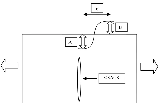
the lateral distance of the peak value as shown in Figure 1.1.

In using such a method for the identification of microcracking several

issues must be investigated. Composites are very stiff materials. It stands to reason that as

the stiffness of a material increases, a larger load would be required to obtain any

noticeable displacements of the surface. Furthermore, the shape and size of a microcrack

is very different than the crack studied in the previous research. A microcrack is a through

crack that is smaller in size in than the 1 inch radius penny-shaped crack studied

previously. Therefore, it would stand to reason that the surface displacements will be

harder to identify.

In this work a finite element analysis is used to study how the loading and

ply lay-up will effect the out-of-plane surface displacement pattern. In addition, several

optical techniques will be investigated. Finally, a discussion will be provided on the

plausibility of using such an approach for the identification of microcracking in

(14)

Figure 1.1 Schematic showing the surface displacement parameters used for characterizing penny-shaped cracks in homogeneous materials

This analysis is limited to cross-ply composites. The microcrack is

considered in the 90° fibers only and is assumed to extend along the entire width of the composite laminate. Simulations are carried out by changing the length of the crack ( i.e.,

the thickness of the inner 90° ply group) and the thickness of the outer ply group. The resulting out-of-plane surface displacements are plotted against the length of laminate.

The following chapter discusses composite materials and types as well as

failures in composite materials, concentrating mainly on failures under transverse loading

(microcracking), several NDT techniques that are used to measure flaws in composites,

and present techniques used to detect microcracking. Chapter 3 focuses on the NDT

approach considered in this research. Chapter 4 provides a description of the finite

element model and analysis created to test the feasibility of utilizing such an approach.

Chapter 5 focuses on presenting the resulting surface displacement patterns for different

lay-ups under investigation. Conclusions and recommendations for future work are

discussed in chapter 6.

B

CRACK A

(15)

2. Literature Review

This chapter begins with a brief discussion of composites and types of

composite failures, concentrating on the onset and progression of microcracking. A

number of non-destructive testing techniques are also discussed in this chapter. Finally,

techniques that have been used to identify microcracking are discussed.

2.1 Composites

A composite material is a macroscopic combination of two or more

physically and/or chemically distinct, suitably arranged or distributed phases with an

interface separating them. Composites are not only used for improving structural

properties, but also for electrical, thermal, environmental properties. They have

characteristics that are not depicted by any of the components in isolation. Modern

composite materials are usually optimized to achieve a particular balance of properties

for a given range of applications. The resulting composite material exhibits improved

properties. The improved structural properties generally result from the load sharing

mechanism. Typically, reinforcements are stronger and stiffer materials and the matrix

acts to hold the fibers together. There are certain exceptions like rubber modified

polymers, where reinforcements are more compliant and more ductile than the polymer,

(16)

According to Miracle and Donaldson (ref 6) composites can be classified at two

levels. The first one is based on matrix constituent. The major classes in this

classification are organic-matrix composites (OMC), metal-matrix composites (MMC)

and ceramic-matrix composites (CMC). Organic-matrix composites include polymer

matrix composites (PMC) and carbon-matrix composites. Carbon matrix composites are

also known as carbon-carbon composites. A second type of classification is based on the

reinforcement form. Particulate reinforcements, whisker reinforcements, continuous fiber

laminated composites and woven composites are grouped into this type of classification.

Generally the volume fraction of reinforcements will be at least 10%. Reinforcement is

considered to be a particle if all dimensions of the reinforcement are equal.

Reinforcements shaped like spheres, flakes and rods of roughly equal axes are grouped in

the particle classification. Whisker reinforcements will have an aspect ratio ranging from

20 to 100. Both of these reinforcements are called as discontinuous reinforcements

because the reinforcements are discontinuous. Other than these reinforcements,

sometimes there are also materials, usually polymers. These are generally referred as

filled systems, because filler particles are included for the purpose of cost reduction.

Continuous fiber reinforced composites will have reinforcement lengths much greater

than their cross sectional dimensions. Most of the fibers in continuous fiber reinforced

composites have lengths that are comparable to the overall dimensions of the composite.

Because of small cross-sectional area, fibers cannot be used in structures directly. Hence

they are embedded in matrix to form fiber-reinforced composites. Matrix binds the fibers

(17)

From Agarwal and Broutman, (1990) [ref 7], fiber-reinforced

composites can be classified as single-layered and multi-layered composites.

Single-layered composites have several distinct layers with each layer having the same

orientation and properties. Most composites used in structural applications are

multi-layered. With multi-layered composites, each layer can be oriented differently. The

directional material properties change based on the orientation of the layers (plies). Each

ply typically has a thickness varying from 0.1-0.2 mm. When the constituent materials in

each layer are the same, though the orientation of fibers is different, they are known as

laminates. These laminates will give improved wear, impact and thermal resistances.

Properties and orientations of the laminae are chosen based on design requirements. Fiber

composites are heterogeneous materials. They fall under the orthotropic material class,

whose behavior lies in between isotropic and anisotropic materials. In general, the

deformation behavior of an orthotropic material is similar to anisotropic material.

However, when loads are applied in axes of symmetry direction, they behave like

isotropic materials.

The final category of composites is formed by weaving, braiding or

knitting the fiber bundles to create interlocking fibers. These fibers will have an

orientation that is orthogonal to primary structural plane. These composites will have

improved properties in the out-of-plane direction.

2.2 Failure in Composites

Failure in fiber-reinforced composites is generally produced by the

accumulation of several types of internal damage. Damage includes fiber breaking,

(18)

on loading and material properties (fiber, matrix and interface). The damage will be

distributed through out the composite and increases with the loading. This damage that is

distributed through out the composite will unite to form a macroscopic fracture before

failure.

Under longitudinal tensile loading failure initiates by fiber breakage at the

weakest cross-section. As the number of broken fibers increases, some cross-section of

composite will become too weak causing complete rupture of the composite. This is

called brittle failure. If the interfaces of broken fibers are debonded because of stress

concentrations created at the fiber ends and thus leading separation of composite at a

given cross-section then that type of failure is called brittle failure with fiber pullout.

Under longitudinal compressive loading fibers act as long columns and

micro buckling may be possible. If fibers are buckled independent of each other then that

mode of buckling is called buckling in extension mode. If they are buckled relative to

each other then that buckling is called buckling in shear mode. Buckling mainly depends

on inter fiber distance

According to J.A.Nairn [ref 8], the first form of damage in composite

laminates with the fibers subjected to a transverse loading is matrix microcracking. These

cracks run through the thickness of ply, parallel to fibers in that ply. These cracks are also

known as matrix microcracks, ply cracks, microcracks, transverse cracks etc. They tend

to develop under tensile, fatigue and thermal loadings. Microcracks usually form in the

plies which are off-axis to the loading direction. These cracks will degrade the thermo-

mechanical properties of the laminate. Upon an increase in loading, these cracks can

(19)

moist air, the micro-cracked laminate will absorb considerably more water than

uncracked laminate. This will then lead to an increase in weight, moisture attack on the

resin and fiber-sizing agents, loss of stiffness, and, with time, an eventual drop in ultimate

properties. In addition, these cracks could possibly link up together or with other types of

damage to produce pathways for leakage.

The formation of the first crack is called the initiation or the onset of

microcracking. Garrett and Bailey (1997), [ref 21] conducted many experiments on

microcracking in [0/90]s laminates made of glass-reinforced epoxy laminates. They

varied the thickness of 90° ply keeping thickness of 0° ply constant. They observed that the thickness of 90° ply has a significant effect on microcrack initiation. They found that as the thickness of the 90° ply is decreased in proportion to the thickness of 0° ply, the strain to microcrack initiation increases. They observed that when the 90°ply thickness is still decreased than 0° ply thickness microcracks are suppressed entirely and the laminate fails before the initiation of any microcracking. Flaggs and Kural (1982), [ref 20]

conducted experiments on microcracking in carbon fiber/epoxy laminates. They also

observed that strain to initiate microcracking increases as the thickness of 90° plies decreases in proportion to the thickness of the 0° plies.

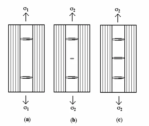
The schematic in figure 2.1 illustrates the progression of microcracking in

the 90° plies of a composite laminate. In general, it is assumed when two microcracks are present that the next microcrack will form halfway between the two that are present. As

shown in schematic 2.1 (b) and (c) a microcrack forms instantaneously at a given load.

(20)

Although the width of the laminate is not shown in this schematic, the microcrack

generally extends through the width as well. Therefore, the microcrack is often thought of

as a rectangular crack possessing the same thickness and width dimensions as that of the

90° ply group.

Figure 2.1. Schematic of microcrack development and progression in 90° ply upon application of transverse loading. (a) Microcrack development at an applied load σ1. (b) Initiation of a microcrack at an

applied load σ2 (σ2>σ1). (c) Progression of microcrack at same applied load σ2.

2.3 Non-Destructive Testing

According to Bray and Stanley (1997) [ref 9], NDT techniques are

characterized as active and passive, or surface and volumetric. In active techniques some

form of energy will be introduced into the specimen and the output energy is measured. If

there are any flaws then a notable change in the input energy can be expected. Eddy

current, magnetic, ultrasonics, radiography etc will fall into this category. In passive

techniques some kind of reaction is expected from the specimen and by measuring that

(21)

penetrant techniques are of this type. Surface techniques are the techniques in which

flaws nearer to the surface are measured and certain modifications for these techniques

will help in measuring flaws away from the surface. Electro magnetic methods are

usually limited to finding flaws nearer to the surface. Volumetric methods like

ultrasonics, acoustic emissions are useful in measuring the flaws away from the surface.

Factors considered when choosing an appropriate technique are size and

orientation of the flaw, type of material, etc. In general, the detection of small flaws will

need more sophisticated techniques when compared to large flaws. In most cases, prior

defect history of the part will help in selecting the proper NDT technique. Understanding

the operation of each and every technique is necessary before selecting the technique.

Existing NDT methods currently useful for crack detection include acoustic emission,

radiography, ultrasonic inspection, and eddy current inspection.

2.3.1 Visual inspection

With visual inspection, identification of flaws is done visually or by

measuring the dimensions of the specimen. It is useful only for large flaws and chances

of missing smaller flaws are very high. Therefore, this method can be useful at a

macroscopic level not but not microscopically.

2.3.2 Penetrant Inspection

Penetrant inspection is based on the principle of capillarity. In this

method penetrant is accumulated around a discontinuity to create a recognizable

indication of the crack or any other surface opening. Capillary action attracts the

penetrant into the void in a greater concentration than its heavier surroundings. Sufficient

(22)

size and shape. This method is not suitable for nonporous and nonmagnetic materials.

This method can be used for identifying the subsurface flaws or crack openings. A crack

or opening that did not reach the surface would not be identified. Thorough consideration

of the surface and fluid properties and the flaw recognition system are the keys for

success of this technique.

2.3.3 Acoustic emission testing

Acoustic emission testing is a passive technique, which uses elastic

techniques generated by cracks, fiber breaks for identifying the defects. In metals and

concrete these acoustic waves are generated by local stress redistributions associated with

motion of dislocations and cracks. In composites these waves are generated by variety of

actions like cracking, separation of fibers and the matrix. Acoustic emission monitoring

systems simply listen to sounds generated by the material. The emission signal is strain

related. Material conditions effect the transmission of emission signals. For example, in

metals it depends on grain size and in composites distribution of the matrix and fiber.

Acceptance of this method is justified on economic basis due to the

reduced labor. The disadvantage with this technique is that the size of the defects can not

be determined. It is often necessary that these emission sources be inspected by some

other NDT techniques like ultrasonics or radiography for assessing the size.

2.3.4 Ultrasonic Inspection

This technique is based on the principles of reflection and refraction. With

this technique, sound waves of short wavelength and high frequency are used to detect

flaws or measure surface displacements. Ultrasonic waves (frequency should be at least

(23)

waves are measured. These waves are often considered in the form of pulses of energy

rather than continuously excited waves. A transducer, which emits ultrasonic pulses, is

placed on the specimen. Typically transducers are made of piezoelectric materials. These

materials have the behavior of converting mechanical vibrations to electric pulses and

vice versa. The pulses that travel through the object are reflected and refracted by defects

in the object. These pulses are then detected by a receiver, which determines the

existence of defect by loss in signal amplitude.

This method can be applied to any material provided that the material

transmits mechanical vibrations. This method is useful in detecting deep surface flaws

and it also gives the details about the depth of crack. Disadvantages of this technique are

that the test object should be a good conductor of sound, it is not suitable for

complex-shaped materials, and it also needs the transducer to be in contact with object.

2.3.5 Radiography

The basic principle of radiography involves propagating energy from a

source through a test object, and evaluating the energy pattern received on the opposite

side. The emitted radiation energy from the source is made to pass through the object.

The evaluation of the condition of the object is done using the pattern of a series of gray

shades between black and white. A recording plane opposite to the source is used to

record the image. This image is a result of difference in attenuation rates, or absorption,

for various types of matter. An image of a defect will occur on the recoding plane (film),

provided that there is a sufficient difference in the radiation intensities received by the

film under the defect as compared to that received through the remainder of the material.

(24)

surroundings. Gamma ray and X ray sources are the typically used radiation energy

sources. The energy level of source can be determined by voltage. High voltage will

result in short wavelength and the amount of current will determine the number of rays

produced.

Radiography is most satisfactory for finding internal, nonplanar defects

such as voids and porosity. Planar defects can also be detected with proper orientation. It

is also useful in detecting changes in material composition. Depth of an object or void

cannot be measured from a single radiographic inspection. The disadvantage of this

technique is that X-rays and gamma rays are hazardous.

2.3.6 Tomography

Tomography is used to reconstruct the interior structural details.

Characteristics such as shape, displacements, internal flaws, and density are measured by

this technique. High quality and very clear cross sectional images can be produced with

this technique. According to Schilling et. al. [ref 12], in this technique an image of the

specimen is recorded to analyze the internal structure. A number of two-dimensional

images are gathered by rotating either the source and detector assembly or by rotating the

specimen, in order to construct a 3-D image. Tomography has a wide range of

applications in medical and ceramic fields.

The main parts in a tomography set-up are a source, a collimator, and a

receiver. The test specimen is placed between the source and the receiver (imaging

system). X-rays are allowed to transmit through the specimen and the receiver measures

the total radiation reached through the object. Images are created, due to the difference in

(25)

will be stored in the memory. After the initial scan the source-detector assembly (or the

specimen holder) will be rotated through a very small step of angle and the procedure

continues for a number of such rotation angles through a total of 180° as it covers the

entire object. This process is called data acquisition. After acquiring data image

reconstruction will be done. If an unknown object is present inside the specimen a change

in absorption can be noticed in the image. This image is stored in the memory.

Reconstruction mainly contains estimation of attenuation for each image from projection

data. As the object is rotated through a small angle, a new image is formed. All these

images are combined to localize the position of absorption point inside the area of

reconstruction. This process is called “back-projection”. With increase in number of

shadow projections, position and shape of absorption can be estimated accurately. Hence

in ideal case, infinite number of projections should result in exact shape. But at the same

time a blur image around the point of absorption is formed because of superposition of

lines will be formed. The process of elimination of the blur area in the back projection

process is known as convolution. All cross-sectional shadows formed along the length of

specimen are combined to get the exact shape and size of the specimen.

As mentioned earlier computed tomography is a specialized technique of

radiography. If X-ray computed tomography results in very high resolution then it can be

called microtomography. With microtomography a spatial resolution of few microns can

be obtained. The main limitation of this process is the small size of the specimen and the

(26)

2.3.7 Eddy current inspection

In this technique eddy currents are induced in the test object by changing

the magnetic field near to it. Changing the current in a conductor creates this magnetic

field. Eddy currents created in test object will generate another magnetic field, which will

oppose the original one. These fields are detected by electro magnetic induction in a coil

or by sensors. In many cases same coils are used to create these eddy currents and also to

detect these fields. The presence of a flaw increases the resistance to the flow of eddy

currents. This change is electronically analyzed to provide the information about type of

flaw, flaw severity or material condition information. This technique can be used for

conductive materials only. This is not useful in giving the exact size and shape of the

defect.

2.4 Identification of Microcracking

The most popular and conventional method for gathering microcracking

information about a specimen involves cutting through the thickness of the composite and

using an optical microscope to view the microcracks. A few NDT techniques have also

been reported in the literature that identify microcracking. These include radiography,

ultrasonics, and microtomography.

Vikram and Lagoudas [ref 11] conducted experiments on cracked

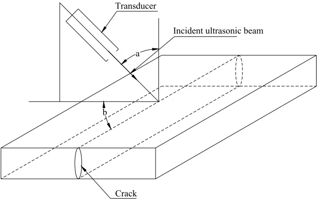
specimens using a polar back scattering technique. Fig 2.3 and 2.4 illustrates the general

configuration of polar back scattering technique. A transducer is used to generate

ultrasonics. The ultrasound is reflected by the crack and ply boundaries back to receiver.

In this case the transducer itself is the receiver. The incident ray is reflected back towards

(27)

to the crack faces. Fig 2.4 better depicts this phenomenon. The transducer receives the

backscattered signal only when the plane containing crack and the plane containing the

transducer axis are perpendicular to each other.

0°

90°

0° Ultrasonic Transducer

Crack

Laminate

Fig 2.3 Schematic of ultrasonic polar backscattering technique.

a

b

Crack

Incident ultrasonic beam Transducer

(28)

Several researchers have identified microcracks in laminates using

radiography. However, because radiographs yield a two-dimensional image, deciphering

the microcracking data contained in each ply is not feasible. Larson et al. (1999) [ref 1]

used microtomography to detect microcracking in [0/90]s laminates. In that work, the

(29)

3 NDT Approach

As mentioned in the introduction, the long-term goal is to develop another

NDT technique that would be useful in characterizing microcracking in composite

laminates. Again, this technique was originally proposed by Larson et al. (1999) [ref 1]

for use on homogeneous materials and is a coupled experimental and computational

technique. An optical technique is used to gather surface data, while a computational

technique is responsible for assessing the internal flaws based on the surface data. The

next section is dedicated to proposing an experimental method that may be used to

induce surface deformations in cracked specimens while the final section discusses some

possible optical techniques that may be used to gather these displacements.

Prior to conducting experiments, a finite element analysis of the procedure

could deem useful in determining if the surface displacement data is on the same order of

magnitude as those that can be resolved by present optical techniques. This issue is the

focus of this report. Chapter 4 is dedicated to the development of such a model and

chapter 5 is dedicated to presenting the magnitudes of the surface displacements for a

number of cross-ply laminates subjected to load limits of 1000MPa and discussing the

plausibility of this proposed experiment.

3.1 Proposed Experiment

The following steps outline the experimental procedure, which will be

(30)

characterize microcracking in composite laminates. The first step involves gathering

specimens with known microcracks in them. Verges et al. (2003) [ref 4], uniaxially tested

a number of IM7/977-2 [0/90]s laminates at specified loads in a tensile substage to obtain

crack density versus load data. The substage used in that work is pictured in Figure 3.1.

Each of these specimens was then inspected via microtomography for microcracking.

Some of these specimens having only a couple of microcracks in them will be used in the

initial tests. IM7/977-2 [0/90/90]s and [0/0/90/90]s specimens will also be loaded and

examined for microcracks via microtomography.

Figure 3.1 Tensile substage used to load the specimen

The second step involves loading these cracked specimens in the tensile

substage. In the work done by Larson et al. (1999) [ref 1], microcracks did not initiate in

the specimens until a load of 1100 MPa was reached. In order to insure no additional

microcracking, the maximum loading on the [0/90/90/0] specimens will be limited to

(31)

The third step involves utilizing an optical technique to measure the

resulting surface deformation. As mentioned in the introduction, composites are very stiff

materials and quite large loads are needed to induce any recognizable surface

deformation. The following section in this chapter discusses possible optical techniques

that may be used in gathering this information. Keep in mind that all of these techniques

can be used in real time; i.e., the surface of the composite laminate will be examined as it

is being loaded.

3.2 Optical techniques

Optical techniques have high sensitivity and full field analysis of inspected

area. As with other NDT techniques, the components are inspected with out any physical

contact. Unlike other NDT techniques, the information used in the analysis of the object

under investigation is gathered from the surface. Therefore, only access to a surface of

the specimen is required.

The main features of optical NDT techniques are non-contact, full-field,

no initial preparation of the object (except in some cases where coating to the object is

helpful) and no real time consumption of films etc. The main optical NDT methods

include the moiré method, holographic interferometry, shearography and photogrametery

[ref 15]. With the exception of the moiré technique, which is limited to obtaining in-plane

surface displacement data, all of these techniques can be used to obtain out-of-plane

surface data. Holographic interferometry, shearography, and photogrammetry will

therefore be discussed a bit further in terms of basic principles, types of measurements,

(32)

3.2.1 Holographic Interferometry

Holography is the method of storing and regenerating all the

amplitude and phase information contained in the light that is scattered from an

illuminated body. Because all the information is reproduced, the regenerated object beam

is, in the ideal case, indistinguishable from the original. Since it is possible to record the

exact shape and position of a body in two different states, movement or deformation can

be measured.

When two beams of coherent light are made to intersect, the interference

between the two beams causes the creation of a three dimensional pattern of interference

fringes. The object beam and reference beam (a plane beam) are the two beams used for

interference. As the plane wave and the object beam merge, they interact to create an

interference pattern. Fringe pattern may be obtained at any particular cross-section by

inserting a photographic emulsion on a plate or film. The optical system should remain

stable enough so that the film is exposed to a stationary pattern. These interference

fringes have a spatial frequency ranging from 2000-3000 lines/mm. The interference

pattern on the film record can only be examined under high magnification. The

photographic record of the wave interference pattern produced by two beams is called a

hologram because it contains all data about the object and reference beams.

The basic idea of holographic interferometry is that the image formed in

holography can be compared with another holographic image of that object. Holographic

interferometry mainly contains two types of recording. First type is “frozen fringe” or

double exposure. In this type of recording, recording medium contains the initial image

(33)

fringe pattern in the form of zebra markings is observed. The other type of recording is

“real time” or “live fringe” recording. In this type of recording, recording medium is

inserted back after the processing of the initial image. These markings will give the

measure of dimensional changes in the object. If the object is disturbed by stress or

moved a small amount then a pattern of interference fringes are formed. By counting

those fringes and comparing with the initial image, the amount of displacement can be

estimated. In traditional holography, the sensitivity of the system is on order of

wavelength of the light and is usually a few tenths of a micrometer. In digital holography,

the sensitivity is reported to be on the order of 10 nm [ref 15].

3.2.2 Shearography

Digital Shearography is an optical interferometric technique that measures surface

strains caused by thermal or mechanical loading. Shearography inspects a full area

simultaneously which is illuminated with a divergent laser beam. It is an optical method,

which measures the derivatives of out-of-plane surface displacements. Hence it is easier

to correlate defects with strain anomalies using shearography than displacement

anomalies applying holography.

A digital shearography set-up is shown in figure 3.2. Just like with

holography, there are two main steps in obtaining any shearographic measurement. The

first step involves grabbing an the image before the object is loaded and the next one

(34)

Figure 3.2 Schematic of a shearography set-up.

The object is illuminated with a coherent laser light inclined at a small

angle to the surface and viewed through an image shearing device like Michelson

interferomer. The effect of shearing is to map a point on the object into two points in the

image. Introducing a glass wedge in front of the camera will shift the rays emanating

from a point on the object away from the normal focal point of the lens as shown in

(35)

Figure 3.3 Schematic showing creation of lateral sheared images.

As the result of shearing action, the light reflected from the object is

sheared or split, causing two separate images with slightly different path lengths from

adjacent areas to be focused on the CCD as shown in figure 3.4. Reflected light from

small adjacent portions of the total surface area is focused on each individual pixel. As

illumination intensity of the light is constant, the intensity of light on each pixel will

depend on the surface and shape of the object. Since each pixel gathers light from only a

small portion of the field of view, the interference pattern is captured and recorded pixel

by pixel in the computer, covering the entire field of view.

As the load is applied on the test object, it will cause change in the shape

of the object and change the path length from point on the surface to each pixel on

camera. The change in path length will cause a new intensity at each pixel, generating a

(36)

Figure 3.4 Schematic showing images being recombined.

Comparison of the two images gives the relative deformation at each point

on the object. Sensitivity of this technique is almost in the same order as of holographic

interferometry. A constant change in surface geometry represents no local deformation.

The direction of shearing can be controlled by rotating the wedge in front of the camera

lens or by tilting the mirror. This technique can be used successfully for complex shapes.

But interpretation of results is not easy and the component must be loaded to see any kind

of result. Only the gradient of deformation is measured.

3.2.3 Photogrammetry

The basic principle used in photogrammetry is triangulation. Photographs

are taken from at least two locations. The line joining the camera position and object

point is called line of sight. These lines of sight are intersected mathematically to get

(37)

metrology. Photography deals with the principles of photogrammetry and metrology is

used for producing 3-dimensional coordinates from two-dimensional photographs.

Photography converts the real 3-dimensional objects into two-dimensional

pictures. Hence some information about the object is lost, usually the third-dimension

information. Photogrammetry maps the two-dimensional images back into 3-dimensional

pictures. For this construction at least two pictures are needed. As the number of pictures

used is increased, the dimensions of the object can be measured more accurately [ref 18].

The object under load is viewed by one or more cameras. A random or

regular pattern with good contrast is applied to the surface of the test object, which

deforms along with the object. The deformation under the load is recorded by CCD

cameras and evaluated. Using photogrammetrical principles the 3D coordinates of the

entire surface of the specimen are calculated. The 3D shape and deformations can be

measured simultaneously. As long as the object remains with in the field of view of the

cameras, all of the local deformations can be tracked. Sensitivity of this technique

depends on field of view. For a 10 x 8 mm field of view sensitivity of this technique is

around 0.3 microns, i.e. 300 nm [ref 19]. Note that the field of view can be altered

(38)

4 Finite Element Analysis

The finite element analysis of the model used in this study is a static,

linear elastic analysis. ANSYS 8.0® finite element software is used for the finite element

work performed and presented here. Appendix A contains the Ansys code used to

perform the finite element analysis on a [0/90/90/0] laminate.

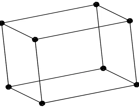
4.1 Model Geometry

The composite laminate modeled in this analysis is similar in geometry to

the composite laminates tested by Larson et al. (1999) [ref 1]. As shown in figure 4.1, the

reference laminate consists of [0/90]s plies. As with the laminates tested by Verges et al.,

the width of laminate is considered to be 5 millimeters. In accordance with the thickness

of the plies tested, the baseline thickness of each ply in the model is taken to be 0.127

mm. Finally, the length of the laminate is taken to be 25.4 mm.

Because the loading on the laminate is symmetric about the plane of the

microcrack, the actual finite element geometry is a quarter model of the laminate. As

depicted in Figure 4.2, the quarter model is created such that the center of the microcrack

is located at the left bottom-most point of the model. The corresponding dimensions are

shown in figure 4.2. Global X, Y and Z axes are taken along the model length, height

(thickness of the plies) and width. S.I. units are used in the analysis.

The quarter model depicted in Figure 4.2 consists of two layers. Each

layer represents a ply of 0.127 mm thickness. The upper layer consists of fibers in 0º

(39)

particular geometry is representative of the reference case. Other cross-ply geometries

were also tested. In each

12.70 0.127

5.00

Fig 4.1 Schematic of [0/90] s composite laminate with microcrack in 90º plies.

case the microcrack is assumed to exist in the center of the laminate thickness. The

thickness of each ply is 0.127 mm. Finally, it is assumed that for cases in which the 90º

plies are adjacent to each other, the microcrack extends through the entire ply group.

4.2 Material Properties

In the work performed byLarson et al. (1999) [ref 1], three different types

of fiber/resin systems were used. One of the material systems tested consisted of IM7

fibers with a 977-2 resin. The material properties used in this work are reflective of an

IM7/977-2 material system. In the designed quarter model, PLY1 is considered to be the

composite ply in which the fibers are oriented 90º to the applied load. As such, the ply is

the stiffest in the z-direction (across the width of the laminate). Hence the material

(40)

9.43x103 N/mm2, 9.43x103 N/mm2 and 159x103 N/mm2, respectively; the Poisson’s

ratios in the xy, yz and xz planes are 0.456, 0.253 and 0.253, respectively; and the shear

moduli in the xy, yz and xz planes are 2.57x103 N/mm2, 4.34x103 N/mm2 and 4.34x103

N/mm2_{, respectively. PLY 2 is considered to be the composite ply in which the fibers are}

oriented parallel to the applied load. As such, the ply is the stiffest in the x-direction.

According to choi and Sankar (2003) [ref 2], Young’s moduli in the x, y and z directions

are 15 x103 N/mm2, 9.43x103 N/mm2 and 9.43x103 N/mm2, respectively. Poisson’s ratios

in the xy, yz and xz planes are 0.253, 0.456 and 0.253, respectively. Shear moduli in the

xy, yz and xz planes are 4.34x103_N/mm2_{, 2.57x10}3_N/mm2_{and 4.34x10}3_N/mm2_,

respectively [ref 2].

4.3 Meshing

Solid 45 elements possess the ability to include complex curve shapes

without loosing accuracy. This element type is often preferred compared to other solid

elements in ANSYS [ref 5]. Solid 45 is used for the three-dimensional modeling of solid

structures. Eight nodes having three degrees of freedom at each node define the element.

These solid 45 elements are used to generate the mesh for the entire model with the

exclusion of the vicinity around the crack tip. Solid 95 elements are used around the

(41)

30

Figure 4.2 Schematic of a 8-noded solid 45 brick element.

Figure 4.3 Schematic of a 20-noded solid 95 brick element.

Singular elements are always preferred around the vicinity of the crack tip.

At the crack tip, four sided elements (in 2-D problems) are often degenerated down to

triangles; for 3-dimensional problems, brick elements are degenerated into wedges. In

elastic problems, the nodes at the crack tip are tied and the mid-side nodes are moved to

(42)

enhances numerical accuracy. A similar result can be achieved by moving mid-side

nodes to quarter points in a four-sided element. But the singularity would only exist on

the element edges; triangular elements are preferred in this case because the singularity

exists with in the element as well as edges. The element is degenerated to a triangular one

as in the case of elastic problems, but the crack tip nodes are united and the location of

mid side nodes are unchanged. This element geometry produces 1/r strain singularity,

which corresponds to the actual crack tip strain field for fully plastic, non-hardening

materials.

For crack tip problems, the most efficient mesh design has proven to be

the “spider web” configuration, which consists of concentric rings of four-sided elements

that are focused towards the crack tip. The innermost ring of elements is degenerated to

triangles. Since the crack tip region contains steep stress, strain gradients with the mesh

refinement should be greatest at the crack tip. As per T.L.Anderson (2002) [ref 3], the

spider web facilitates a smooth transition from a fine mesh at the crack tip to coarser

mesh remote to the tip. Nodes are generated at their respective places and then elements

are generated from nodes. Therefore, in this analysis, the mid-points are generated for the

solid 45 elements, around the crack tip and then moved to the quarter distance. This is

achieved by using a macro in the ANSYS program. The mesh at the crack tip for the

quarter model is as shown in figure 4.4. An isotropic view of the entire mesh used in the

(43)

1

X

Y

Z

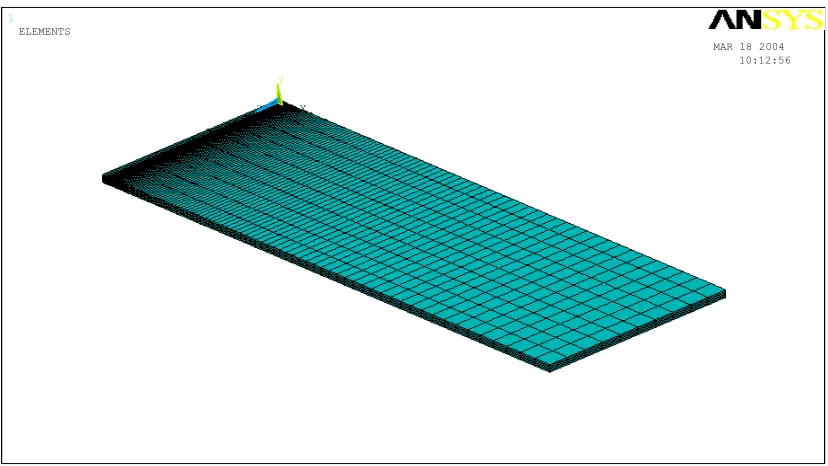
APR 20 2004 16:46:58 ELEMENTS

MAT NUM

Figure 4.4 Two-dimensional view of the mesh around the vicinity of the crack tip. The crack tip is located at the center of the left-most edge.

1

X Y

Z

MAR 18 2004 10:12:56 ELEMENTS

(44)

4.4 Boundary conditions

Due to symmetry conditions, the nodes on the plane corresponding to y =

-0.127mm in figure 4.6, are constrained from moving in the y-direction. (Note here that

the origin of the coordinate system is located at the crack tip.) Similarly the nodes on the

plane corresponding to z = 2.5 mm are constrained from moving in the z-direction. (This

plane is located across the center of the laminate width.) The nodes corresponding to the

plane where x = 0 in the upper ply are also constrained in the x-direction. To simulate the

microcrack, the nodes on the plane of the lower ply at x = 0 are allowed to move freely in

all directions.

1

X Y

Z

APR 20 2004 16:52:36 ELEMENTS

MAT NUM

U

PRES-NORM -1000

(45)

4. 5 Loading

It was stated in chapter 3 that complementary research is underway in which a

tensile substage is being used to load IM7/977-2 [0/90/90/0] specimens. To simulate this

type of uniaxial loading in the finite element model, a pressure load varying from 250

MPa to 1000 MPa is applied at the surface formed by nodes on the plane x = 12.7 mm.

This loading condition is shown in figure 4.7.

The magnitude of the loading applied to the laminate must be high enough

to obtain substantial out-of-plane displacements at the surface; however, this loading can

not be arbitrary. Recall that the goal is to identify microcracking that already exists, not

to induce more microcracking. Again, the reference laminate for this work is the

[0/90/90/0] laminate used by Larson et al. (1999) [ref 1]. In that work, microcracking

was initially identified at a loading of 1100 MPa. Therefore, in the analysis, the highest

(46)

1

X Y

Z

APR 20 2004 20:29:44 ELEMENTS

MAT NUM

U

PRES-NORM -1000

Figure 4.7 Location of force (depicted by red arrows) on the quarter model of the [0/90/90/0] laminate.

4.6 Solution Convergence Testing

Finer meshes were generated for testing the convergence of solution. A finer

mesh means more number of elements, which in turn means more degrees of freedom. In

this analysis the number of degrees of freedom is increased from 51156 to 80640 for

[0/90] s laminate, at a load of 1000 MPa. Each time Uy at the mid-plane is plotted against

nodal distance. From figure 4.8 it is evident that the Uy solution is converged from along

the length of the model for a D.O.F of 51912. Hence for this analysis the number of

degrees of freedom used is 51912. When changing the number of degrees of freedom, the

nodes at the crack tip in the spider web configuration are changed from four to ten. For

(47)

crack tip are kept equal to the number of nodal divisions at y=0 in the spider web. Six

nodes at y=0 in the spider web gave same results as 8 nodes and 10 nodes. Hence number

of nodes in the spider web and number of elements around the crack tip are taken as

six.

(48)

5. Results

Figures 5.1(a) and 5.1(b) show the effect of width on out-of-plane

displacements on a section taken near the vicinity of the microcrack for the [0/90/90/0]

laminate. The widths of the laminate considered here are 5mm and 10mm. Note for the

same 1000MPa loading that edge effects can be observed in both cases. In figures 5.1(a)

and 5.1(b) a different displacement contour can be seen at the edges of the laminate,

which describes the edge effect. It is evident from the figures that edge effects do not

effect the out-of-plane displacements along the xy mid-plane.

1

MN MXX Y

Z

-.00161 _-.00158 -.0014 _-.00138 -.00128 _-.00108 -.808E-03 _-.608E-03 -.308E-03

APR 24 2004 13:38:07 NODAL SOLUTION STEP=1 SUB =1 TIME=1 /EXPANDED UY (AVG) RSYS=0

DMX =.01244 SMN =-.00161 DSYS=11

Figure 5.1(a) Out-of plane contours on the top surface of a [0/90/90/0] laminate with a microcrack extending through both 90 plies and a transverse loading of 1000 MPa. This picture shows the top view of a

5mm wide laminate. Here a 2mm section in length is shown with the microcrack located in the center. The top boundary represents the edge of the laminate while the bottom boundary represents the mid-plane. Each

(49)

1

MN MXX

Y

Z

-.00158 -.00148 -.00138 -.00128 -.00118 -.00108 -.808E-03 -.608E-03 -.308E-03

APR 24 2004 13:23:37 NODAL SOLUTION STEP=1 SUB =1 TIME=1 /EXPANDED UY (AVG) RSYS=0

DMX =.012556 SMN =-.00158 DSYS=11

Figure 5.1(b) Out-of plane contours on the top surface of a [0/90/90/0] laminate with a microcrack extending through both 90 plies and a transverse loading of 1000 MPa. This picture shows the top view of a

10 mm wide laminate. Here a 2mm section in length is shown with the microcrack located in the center. The top boundary represents the edge of the laminate while the bottom boundary represents the mid-plane.

Each contour represents an interval of 100 nanometers.

The nodal solution for Uy (out-of-plane displacement) in the [0/90]s 5 mm

wide laminate along the xy mid-plane (located on the plane where z=2.5mm) for a load of

1000 MPa is shown in figure 5.2. In this figure the results have been symmetrically

expanded about the yz and xz planes to show the out-of plane displacements surrounding

the microcrack. The figure only shows a 2mm length section of the laminate. In this

figure each contour represents an interval of 175 nanometers. In the following analysis,

the out-of-plane surface displacements on the xy mid-plane are considered for the

(50)

1

MN MX

-.001213_-.001078-.943E-03_-.809E-03-.674E-03_-.539E-03-.404E-03_-.270E-03-.135E-03₀

MAY 3 2004 01:26:05 NODAL SOLUTION

STEP=1 SUB =1 TIME=1 /EXPANDED UY (AVG) RSYS=0

DMX =.012635 SMN =-.001213 DSYS=11

Figure 5.2Uy nodal solution at the xy mid-plane for a section length

of x = -1 mm to 1 mm for a [0/90/90/0] laminate with a microcrack extending through the 90 plies and a transverse loading of 1000 MPa. In this graph each contour represents 100 nanometers.

(51)

In the work performed by Herrington et al. (2002) [ref 13] on penny-shaped cracks in

homogeneous materials subjected to a transverse loading, several surface parameters

were identified and analyzed with respect to two crack parameters (radius and crack

depth). Following this procedure, the surface displacement parameters depicted in figure

5.3 (a) are used in the current analysis. In this figure, (Uy)o denotes the constant far-field

y-displacement value, (Uy)p denotes the peak value, (Uy)m denotes the minimal value,

(Ux)p denotes the lateral distance of the peak value from the center of the microcrack and

(Ux)o denotes the lateral distance of the constant far-field value from the center of the

microcrack. The parameters associated with cracked specimen are a bit more complex

due to the heterogeneous nature of the composite laminate. Figure 5.3 (b) denotes the

laminate parameters considered in this work. Again, recall that for each case tested the

microcrack exists in the center of the specimen and extends through the thickness of the

90º ply group. (It also extends through the entire width.) As shown in the schematic, the

half-thickness of the microcrack is represented as a. The depth of the microcrack here is

considered to be the distance from the laminate surface to the crack tip to the center of

the microcrack and is denoted as d. Note that for all cases tested this depth is equal to the

half-thickness of the laminates. A third parameter dct denotes the distance from the

surface to the crack tip (dct =d-a). Because these laminates are not homogeneous two

other parameters dealing with the make-up of the laminate have been identified. The first

parameter deals with the ratio of 90º plies to 0º plies and is denoted as Tp. For example,

for a [0/90]s laminate the ratio is 1/1 and for a [0/0/0/90]s the ratio is 1/3. The second

(52)

Dp. (In figure 5.3 (b) the dct region is highlighted in yellow.) For example, for a [0/90]s

laminate, Dp=0, and for a [0/90/0/90]s laminate Dp=1/2.

Eleven different IM7/977-2 cross-ply laminate configurations were analyzed in

this research. Recall from chapter 4 that each ply has a constant thickness of t =

0.127mm. The mesh for the [0/90]s laminate is depicted in figure 4.4. This reference

mesh was used in each of the other ten meshes to be the mesh around the crack tip.

(a)

(b)

(53)

When adding outer plies to the finite element geometry, nodes on the top

surface of the reference mesh are copied that many times depending on number of plies

and are joined by rectangular elements. A similar procedure is followed for adding more

inner plies, using the bottom surface of the reference mesh. Meshes used for [0/0/90]s and

[0/90/90]s are shown in figures 5.4(a) and 5.4(b). The boundary conditions, material

properties, and loading conditions are also modified each time to reflect the appropriate

behavior of the laminate. For each laminate transverse loadings of 250MPa, 500MPa, 750

MPa, and 1000 MPa were applied. Table I summarizes the resulting surface data in terms

(54)

1

X Y Z

APR 30 2004 00:31:16 ELEMENTS

MAT NUM

Figure 5.4 (a) Mesh of the [0/0/90]s laminate.

1

X Y

Z

APR 30 2004 00:32:40 ELEMENTS

MAT NUM

(55)

Table I. Surface Parameter Values for Different Ply Orientations and Loadings.

Laminate

Number Ply Orientation Loading (MPa) (Ux)(mm) p (Uy)(nm) p (Uy)(nm) m (Uy)(nm) p–(Uy)m (Uy)(nm) o (Ux)(mm) o

1 [0/90]s 250 0.16 -242 -282 40 -303 0.55

a=t d=2t 500 0.16 -483 -563 80 -607 0.55

dct=t 750 0.16 -726 -844 118 -910 0.55

Tp=1 Dp=0 1000 0.16 -968 -1126 158 -1214 0.55

2 [0/90/90]s 250 0.31 -454 -725 271 -676 1.05

a=2t d=3t 500 0.31 -907 -1451 544 -1352 1.05

dct=t 750 0.31 -1361 -2176 815 -2027 1.05

Tp=2 Dp=0 1000 0.31 -1814 -2901 1087 -2703 1.05

3 [0/90/90/90]s 250 0.42 -687 -1430 743 -1165 1.49

a=3t d=4t 500 0.42 -1373 -2860 1487 -2331 1.49

dct=t 750 0.42 -2060 -4290 2230 -3496 1.49

Tp=3 Dp=0 1000 0.42 -2746 -5720 2974 -4662 1.49

4 [0/90/90/90/90]s 250 0.55 -937 -2398 1461 -1755 1.92

a=4t d=5t 500 0.55 -1874 -4796 2922 -3510 1.92

dct=t 750 0.55 -2811 -7194 4383 -5266 1.92

Tp=4 Dp=0 1000 0.55 -3748 -9592 5844 -7020 1.92

5 [0/0/90]s 250 0.16 -296 -303 7 -333 0.51

a=t d=3t 500 0.16 -593 -606 13 -666 0.51

dct=2t 750 0.16 -890 -909 19 -999 0.51

Tp=1/2 Dp=0 1000 0.16 -1186 -1211 25 -1332 0.51

6 [0/0/0/90]s 250 0.13 -357 -358 1 -386 0.42

a=t d=4t 500 0.13 -714 -716 2 -771 0.42

dct=3t 750 0.13 -1071 -1073 2 -1156 0.42

Tp=1/3 Dp=0 1000 0.13 -1428 -1431 3 -1541 0.42

7 [0/0/0/0/90]s 250 - -418 -418 0 -442 0.30

a=t d=4t 500 - -836 -836 0 -884 0.30

dct=3t 750 - -1254 -1254 0 -1326 0.30

(56)

Laminate

Number Ply Orientation Loading (MPa) (mm) (Ux)p (Uy)(nm) p (Uy)(nm) m (Uy)(nm) p–(Uy)m (Uy)(nm) o (mm) (Ux)o

8 [90/0/0/90]s 250 0.16 -564 -566 2 -607 0.30

a=t d=4t 500 0.16 -1128 -1132 4 -1214 0.30

dct=3t 750 0.16 -1692 -1698 6 -1821 0.30

Tp=1 Dp=1/2 1000 0.16 -2256 -2264 8 -2428 0.30

9 [90/0/90]s 250 0.16 -605 -623 18 -676 0.38

a=t d=3t 500 0.16 -1212 -1247 35 -1352 0.38

dct=2t 750 0.16 -1818 -1870 52 -2028 0.38

Tp=2/3 Dp=1 1000 0.16 -2423 -2494 71 -2704 0.38

10 [0/0/90/90]s 250 0.34 -484 -565 81 -607 1.05

a=2t d=4t 500 0.34 -968 -1130 162 -1214 1.05

dct=2t 750 0.34 -1451 -1695 244 -1821 1.05

Tp=1 Dp=0 1000 0.34 -1935 -2260 325 -2428 1.05

11 [0/90/0/90]s 250 0.12 -566 -567 1 -607 0.38

a=t d=4t 500 0.12 -1131 -1134 3 -1214 0.38

dct=3t 750 0.12 -1697 -1701 4 -1821 0.38

Tp=1 Dp=1/2 1000 0.12 -2252 -2267 15 -2428 0.38

Far-field Uy Values

When comparing the far-field y-displacement values for all eleven cases in

Table I for any given load the biggest deformation occurs in case 4 for a [0/90/90/90/90]

laminate and the smallest value occurs in case 1 for a [0/90]s laminate. It is obvious from

the table that the values are dependent on the laminate thickness, d, as well as the ratio of

90º plies to 0º plies. This trend is expected since the far-field y-value is dependent on

laminate geometry and not the microcrack. For cases 2 and 9 the far-field values are

equal. This is expected since both laminates have the same laminate thickness and the

same number of 0º and 90º plies. The same is true for cases 8, 10, and 11. Also, note that

Investigation of Surface Displacements Induced in Loaded Cross-Ply Composite Laminates with Microcracking

ScholarWorks@UNO

ScholarWorks@UNO

Investigation of Surface Displacements Induced in Loaded

Investigation of Surface Displacements Induced in Loaded

Cross-Ply Composite Laminates with Microcracking

Ply Composite Laminates with Microcracking

INVESTIGATION O

F

SURFACE DISPLACEMENTS INDUCED IN

LOADED CROSS-PLY COMPOSITE LAMINATES WITH

MICROCRACKING

Acknowledgements

Table of Contents

List of Figures

LIST OF TABLES

Abstract

Introduction

2. Literature Review

3 NDT Approach

4 Finite Element Analysis

5. Results