The Search Problem in Mixture Models

(1)

The Search Problem in Mixture Models

Avik Ray [email protected]

Department of Electrical and Computer Engineering University of Texas at Austin

Austin, TX 78701, USA

Joe Neeman [email protected]

Department of Mathematics

Rheinische Friedrich-Wilhelms-Universit¨at Bonn D-53115 Bonn, Germany

Sujay Sanghavi [email protected]

Sanjay Shakkottai [email protected]

Editor:Animashree Anandkumar

Abstract

We consider the task of learning the parameters of asinglecomponent of a mixture model, for the case when we are given side information about that component; we call this the “search problem” in mixture models. We would like to solve this with computational and sample complexity lower than solving the overall original problem, where one learns parameters of all components.

Our main contributions are the development of a simple but general model for the notion of side information, and a corresponding simple matrix-based algorithm for solving the search problem in this general setting. We then specialize this model and algorithm to four common scenarios: Gaussian mixture models, LDA topic models, subspace clustering, and mixed linear regression. For each one of these we show that if (and only if) the side information is informative, we obtain parameter estimates with greater accuracy, and also improved computation complexity than existing moment based mixture model algorithms (e.g. tensor methods). We also illustrate several natural ways one can obtain such side information, for specific problem instances. Our experiments on real data sets (NY Times, Yelp, BSDS500) further demonstrate the practicality of our algorithms showing significant improvement in runtime and accuracy.

Keywords: mixture models, search, side information, semi-supervised, method of mo-ments

1. Introduction

Mixture models denote the statistical setting where observed samples can come from one of several distinct underlying populations—each typically with its own probability distribution—

c

(2)

but are not labeled as separate in the data presented. They have been used to model a wide variety of phenomena, and have seen great success in practice, going back as far as Pear-son (1894). In this paper we consider (what we call) the search problemin the mixture model setting: given some special side information about one of the mixture components, is it possible to efficiently learn the parameters of that component only? Given that there are known methods for learning the entire set of parameters of various mixture models, “efficient” here means more efficient (statistically and/or computationally) than existing methods for learning all the parameters.

As an example, we consider the “latent Dirichlet allocation” model for document gener-ation. In this model, “underlying population” means the set of topics in a document, which determines the frequencies of different words in the document. “Side information” could be a word that is more common in the topic of interest than it is in any other topic: for example, the word “semi-supervised” might work if the topic of interest is machine learning.

Side information could also consist of a small number of labelled examples. We might have a small collection of documents about machine learning and also a much larger corpus that includes documents from many topics. Our methods will allow us to leverage the large, unlabelled corpus to obtain good estimates for word frequencies in machine learning articles—and these estimates will be much better than anything that could be learned from the small labelled sample.

Main contributions: We propose a general setting for side information in mixture models, and show how to solve the search problem by estimating certain matrices of mo-ments. We prove error bounds on the resulting estimates; our rates have a sharp dependence on the sample size (although they are possibly not sharp in the other parameters).

We then specialize our approach to four popular families of mixture models: Gaussian mixture models with spherical covariances, latent Dirichlet allocation for topic models, mixed linear regression, and subspace clustering. We give concrete algorithms for these four families. Our results also include new moment derivations for mixed linear regression and subspace clustering models.

(3)

1.1 Related Work

There is a vast literature on mixture models; too much to even summarize here. We will therefore focus this section on two more closely related areas: method of moments estimators for mixture models, and learning with side information.

Mixture models and method of moments: A common method for learning mixture models is the EM algorithm of Dempster et al. (1977), which outputs a complete set of model parameters. However, EM may converge slowly (or not at all) [Redner and Walker 1984]; this weakness of EM has spurred a resurgence in method-of-moments estimators for mixture models. Although these methods go back to the pioneering work of Pearson (1894) on Gaussian mixture models, the last several years have seen important advances. Moitra and Valiant (2010), and Hardt and Price (2015) showed that Gaussian mixture models with two components can be learned in polynomial time. Hsu and Kakade (2013) considered mixtures of more Gaussians, but constrained to have spherical covariances. They gave a method based on third-order tensor decompositions, which was later generalized to other models in Anandkumar et al. (2014).

Learning with side information: As has been observed many times, often in practice one has access to a set of data that is somewhat richer than standard models of data in learning theory. The termside informationis used as a catch-all for extra data that doesn’t fit into pre-existing models; as such, the literature contains many incomparable models of side information.

Xing et al. (2002) and Yang et al. (2010) took unsupervised clustering as their starting point. For them, side information arrived as pairs of points that were known to belong to the same cluster; they showed how this extra information could substantially improve the performance of the k-means algorithm.

Kuusela and Ocone (2004) developed a framework for side information in the PAC learning model, in which extra samples with a particular dependence on the original samples could sometimes give a substantial benefit.

Many different types of metadata have been proposed for thelatent Dirichlet allocation

(LDA) model of document generation. Mcauliffe and Blei (2008) introduced thesupervised LDA model, in which each document comes with an additional response variable from a generalized linear model. On the other hand Rosen-Zvi et al. (2004) proposed the

author-topic model, in which the metadata (author names) affects the distribution of the documents

themselves. From a more experimental point of view, Lu and Zhai (2008) used long, detailed product reviews as side information for categorizing short snippets and blog entries.

The notion of semi-supervised learning (see the book by Chapelle et al. (2006)) is also related to our framework of side information. In semi-supervised learning, the learner has access to a small number of labelled examples and a large number of unlabelled examples. This setting is useful for us too, although our general method does not strictly require data of this form.

2. Basic Idea and Algorithm

(4)

Setting: We are interested in the standard statistical setting of (parametric) mixture models: that is, samples are drawn i.i.d. from a distribution f given by

f(x) =

k

X

i=1

αig(x;µi).

Here g corresponds to a known parametric class of distributions, and k is the number of mixture components. The corresponding parameter vectors are µ1, . . . , µk, and their

mixture weights / probabilities areα1, . . . , αk. So, for example, in the case of the standard

(spherical) Gaussian mixture model,g(x;µi) is the Gaussian pdfN(µi, I). Thus each sample

can be considered to be drawn by first selecting a mixture component µi with probability

αi, and then drawing the samplexaccording to g(x;µi). We assume all theµi’s arelinearly

independent. This is a common assumption for learning mixture models using spectral

methods.

Search problem: The standard parameter estimation problem is to find all the µi

vectors given samples. In this paper we are interested in the search problem: we are given

side informationabout one of the vectors—sayµ1, without loss of generality—and we would

like to recoveronlyµ1. Of course, we would like to do this with sample and computational complexity lower than what would be required to estimate all parameter vectors (i.e., lower complexity than the standard case).

Side information: Our general procedure requires the following model for side infor-mation: we assume that we have access to a vectorv such that the inner product with the parameter vectorµ1—the special one we are searching for—is higher than the inner product with any of the other µi; i.e. there existsδ >0 such that;

hµ1, vi ≥ (1 +δ)hµi, vi for all i6= 1

Section 3 shows how to obtain such side information in some specific models of interest: spherical Gaussian mixture models, mixed linear regression, subspace clustering and the LDA topic model.

We remark that it’s also possible (and perhaps more intuitive in some situations) to ask for side information satisfying|hµ1, vi| ≥(1 +δ)|hµi, vi|. However, our assumption above is

slightly weaker, since for anyv satisfying the latter assumption, either vor−vsatisfies the former assumption. Later, we show the above condition is sufficient for uniquely identifying the required parameterµ1 (but it may not be necessary). We refer side information vector

v asinformativeabout µ1 if it satisfies the above condition.

2.1 General Procedure

The main idea behind method of moments is to use samples to estimate certain moments of the distribution f(x),using which we can recover the parameters of interest. For many mixture models (including the four common examples we detail), it is possible to easily and directly estimate using first and second order moments, given sufficient samples, the vector

m:=

k

X

i=1

(5)

and the matrix

A:=

k

X

i=1

αiµiµTi . (2)

For example, in many models the estimate of vector m is simply the sample mean, and matrix A can be derived from the sample covariance matrix. The exact procedure for estimating m and A varies according to the particular parametric model g. The fact that m and A (and also higher-order tensors) can be estimated from samples is well known for many models, see Anandkumar et al. (2014) for a treatment of several different models, and for other pointers to the literature.

Typically, all mixture model components cannot be identified from just the first and second order moments (or m and A). It is often necessary to compute even higher order moment terms. In our search problem, given the side information,we developprocedures to estimate an alternative matrixB, using higher order moments, given by

B :=

k

X

i=1

αihµi, viµiµTi (3)

Again, the exact procedure for estimating B from samples depends on the particular para-metric model g.

For this section, we assume we are able to estimateA, B, mto within some accuracy. We will use the notation ˆA,B,ˆ mˆ to denote these finite sample estimates ofA, B, mrespectively, andndenotes the number of samples used to compute these estimates. With this in hand, we outline two general procedures for estimatingµ1 (i.e. the component that we are interested in). The first procedure is based on a whitening step, much like the one that is used in the spectral algorithms in Hsu and Kakade (2013); Anandkumar et al. (2012), and tensor decomposition methods of Anandkumar et al. (2014) (please see remarks in Section 3 for the differences for specific models). The second procedure uses a line search instead, and may be computationally favorable when k is large, because it avoids the need to invert a k×k matrix. Both Algorithms 1 and 2 take as input the estimates ˆA,B,ˆ mˆ (where ˆB is constructed using side information vectorv) and they output estimates of the first mixture component ˆµ1,and also the proportion of the first component ˆα1.

2.1.1 The Whitening Method

Our main result about Algorithm 1 is that if ˆA and ˆB are good estimates ofA and B then Algorithm 1 outputs good estimates for µ1 and α1. In order to interpret Theorem 1 as an error rate, note that if all parameters but are fixed then the error is O(). Since standard concentration results yield =O(n−1/2), where nis the number of samples; our error rate in terms of n is also O(n−1/2_{). This rate is sharp, since it is also the rate for} estimating the mean of a single Gaussian vector (i.e. a GMM with only one component).

Theorem 1 Suppose that µ1, . . . , µk are linearly independent, and that Aˆis positive semi-definite. Also suppose that hµ1, vi ≥(1 +δ)hµi, vi for all i6= 1. Assume that

(6)

Algorithm 1 Extracting a mixture component from side information: the whitening method.

Input: A,ˆ B,ˆ mˆ Output: µˆ1,αˆ1

1: let{σj, vj} be the singular values and singular vectors of ˆA, in non-increasing order 2: letV be the d×k matrix whosejth column isvj

3: letD be thek×k diagonal matrix with Djj =σj 4: letu be the largest eigenvector ofD−1/2VTBV Dˆ −1/2

5: letw=V D1/2u

6: letE be the span of{V D1/2v :v⊥u}

7: write V VT_m_ˆ _{(uniquely) as}_aw₊_y_{, where} _y_∈_E 8: returnw/aand a2

and that the right hand side of (4) is at most α1. Then

kµ1−µˆ1k ≤CR|α −1/2 1 −αˆ

−1/2 1 |+C

p

σ1(A)

√

α1

η , and

|α1−αˆ1| ≤

C√α1(α1R+η) σk(A)

η+R σk(A)

+

(4)

where η = σ1

δσ_k5/2, R= maxikµik, σ1(A)≥ · · · ≥σk(A)>0 are the non-zero singular values

of A=P

iαiµiµTi , andC is a universal constant.

Our error bounds are somewhat complicated, and depend on many different parameters, so let us elaborate on them slightly. First of all, the dependence on σ1(A) and σk(A) is

of the order kµ1−µˆ1k.σ1(A)3/2/σk(A)5/2, which is probably an artifact of the analysis,

and not the true behavior of the algorithm. On the other hand, our dependence on is optimal: we have |α1 −αˆ1| . and kµ1 −µˆ1k . . Note also that our bound has no explicit dependence onk; this feature comes from the fact that our method is targeted at a single mixture component. By comparison, other methods typically give bounds in which

the averaged per-mixture-component error does not depend on k. In terms of dependence

onk, therefore, our bounds are better than previous bounds if there is only one component of interest.

Finally, let us remark on the assumption that the right hand side of (4) is at most α1. This amounts to an assumption that is sufficiently small compared to all the other parameters. Without this assumption, the bound in (4) would not be very interesting, since

|α1−αˆ1| ≤α1 is too weak to give useful information about ˆα1 (it could even be zero). We defer the actual analysis of Algorithm 1 to the appendix, but we will motivate the algorithm and give the basic idea of the proof by showing that if ˆA,Bˆ, and ˆm are equal to A, B and m respectively then Algorithm 1 outputs µ1 and α1 exactly.

Lemma 2 Let m,A, andB be defined by in (1),(2), and (3), where µ1, . . . , µk are linearly

independent. If hµ1, vi >hµi, vi for all i 6= 1 and we apply Algorithm 1 to A, B, and m,

(7)

Proof Let V and D be as defined in Algorithm 1. SinceA has rank k,

k

X

i=1

αiD−1/2VTµiµTi V D

−1/2₌_D−1/2_VT_{AV D}−1/2 ₌_I

k.

Defining ui :=

√

αiD−1/2VTµi, we have PiuiuTi = Ik, which implies that the ui are

orthonormal in Rk. Now,

D−1/2VTBV D−1/2 =

k

X

i=1

αihµi, viD−1/2VTµiµTi V D

−1/2₌

k

X

i=1

hµi, viuiuTi .

Sincehµ1, vi was assumed to be larger than all otherhµi, vi, it follows thatu1 is the largest eigenvector of D−1/2VTBV D−1/2. Now, ifw=V D1/2u1 thenw=

√

α1µ1.

Now, note that since the µi are linearly independent, there is a unique way to write

m=V VTm=P

iαiµ1 asaw+y, wherey belongs to the span of{µ2, . . . , µk}(which is the

same as the span of {V D1/2ui :i≥ 2}. Moreover, the unique choice of athat allows this

representation must satisfyaw =α1µ1, which implies that a=

√

α1. Therefore, w/a=µ1 and a2 ₌_α

1.

The proof of Lemma 2 is crucial to understanding the algorithm, and also the broader message of this article: if we can get hold of two different normalizations of something, then we can learn something about it. In the proof of Lemma 2, this happens twice: first, we use the fact thatA and B contain the same components (but with differing normalizations) to extract the span of a single component of interest. The differing normalization is crucial, because A by itself does not uniquely determine the set{µ1, . . . , µk}, much less single out

a specific component of interest.

In the second step of Lemma 2, we know √α1µ1, which is not enough to determine eitherα1 orµ1. However, we also have access tom, which involves a contribution ofα1µ1. Exploiting the difference between these two normalizations, we recover both α1 andµ1. 2.1.2 The Cancellation Method

Our second method avoids the matrix inversion in Algorithm 1, preferring a line search instead.

In the above Algorithm 2, we assume hµ1, vi >0.When this is not the case and B is a negative semi-definite matrix, we simply have to change the line search step to search for the smallest λ < 0 such that VbVbT(Ab−λBb)VbVbT is PSD. Theorem 3 shows that with

m, A, B estimated up to O() error, the parameter estimation error in Algorithm 2 is also bounded as O().

Theorem 3 Suppose {µ1, . . . , µk} are linearly independent and v satisfies hµ1, vi ≥ (1 + δ)hµi, vi for all i 6= 1. Suppose that max{kAb−Ak,kBb −Bk,kmˆ −mk} < , and λ₁ := 1/hµ1, vi.Then Algorithm 2 returns µˆ1,αˆ1 with

kµˆ1−µ1k < C α2₁a2₁

σ1(A)

1 + α1a1 σk−1(Zλ1)

+ σ1(A)η3R σk−1(Zλ1)

|αˆ1−α1| <

Cσ1(A) α1a31

η1+

η2Rη3 σk−1(Zλ1)

(8)

Algorithm 2 Extracting a mixture component from side information: the cancellation method.

Input: A,ˆ B,ˆ mˆ Output: µˆ1,αˆ1

1: letVb be the d×k matrix ofk largest eigenvectors of ˆA;

2: search over λto find the largestλ=λ∗ such thatVbVbT(Ab−λBb)VbVbT is PSD;

3: letZb_λ∗ =Ab−λ∗B,b and let {v₂, . . . , v_k} be the topk−1 singular vectors of Zb_λ∗

4: letV1:(k−1) be the d×(k−1) matrix with columns {v2, . . . , vk}

5: letx1= ˆm−V1:(k−1)V1:(Tk−1)mˆ

6: letv1 =x1/kx1k

7: computeci =v1TAvb _i fori= 1 tok

8: letai =ci/kx1k fori= 1 to k

9: return ˆµ1=Pk_i₌₁aivi and ˆα1 =c1/a21

where η1 := max{α1a1(2a1+ 1),20}, η2 := max{α1a21,10}, η3 = max{1, λ1, σ1(B)}, R= maxkµik, a1 =kµ1−QVµ1k,where V =span{µ2, . . . , µk},andC is an universal constant.

Again, we will defer the actual analysis to the appendix, and instead show that Algo-rithm 2 returns the exact answer when fed exact initial data. We will do this in two lemmas: Lemmas 4 and 5.

Lemma 4 Let Z =Pk

i=1γiµiµTi where {µ1, . . . , µk}are linearly independent, µi∈Rd, γi ∈ R andd > k. If γ1 <0 and γi >0 for all i6= 1 then Z is not positive semi-definite.

Proof Let Π denote the projection onto the orthogonal complement of span{µ2, . . . , µk}.

Let x = Πµ1, and note that hx, µ1i > 0 but hx, µii = 0 for all i 6= 1. Hence, xTZx =

γ1hx, µ1i2 <0 and soZ is not positive semi-definite.

Lemma 5 Let m,A, andB be defined by in (1),(2), and (3), where µ1, . . . , µk are linearly

independent. If hµ1, vi >hµi, vi for all i 6= 1 and we apply Algorithm 2 to A, B, and m,

then it returns µ1 and α1.

Proof Define wi=hµi, vi and letγi=αi(1−λwi), so that

Zλ=A−λB= k

X

i=1

γiµiµTi .

Note that, in our case where Ab = A, and Bb = B, columns of Vb simply form a common orthonormal bases of the row/column space of both matrices A, B. Therefore the matrix

b

VVbT(A−λB)VbVbT =A−λB =Z_λ.Now forλ > _w11 , γ₁<0 and for allλ≤ _w11 , γ_i ≥0 for all isince w1 > wi,for every i6= 1. By Lemma 4, λ∗ = _w11 is the largestλsuch that Zλ is

PSD; hence,

Zλ∗ = k

X

i=2

(9)

From Lemma 26 in Appendix E.2 it follows that k−1 singular vectors{v2, . . . , vk}of Zλ∗

form a basis of the subspace V = span{µ2, . . . , µk}. Let V⊥ be the perpendicular space of

V, and write Π =I−V1:(k−1)V_1:(T_k−1) for the orthogonal projection ontoV⊥. Since Πµi = 0 fori6= 1, we have x1= Πm=αΠµ1.

Now define b1, . . . , bk by µ1 = Pk_i₌₁bivi. In order to prove that the algorithm returns

µ1 correctly, we need to show that bi=ai :=ci/kx1k. Indeed,

ci :=vT1Avi= k

X

j=1

αjvT1µjµTjvi =α1b1bi,

since v₁Tµj = 0 for j 6= 1. On the other hand, kx1k =αkΠµ1k = αb1, and so bi = ai, as

claimed. Moreover, ˆα1 = _ac12 1

=α1, as claimed.

Optimization for λ∗: The first step of Algorithm 2 involves finding a smallest λ∗ such that Zb_λ0∗ =VbVbT(Ab−λ∗Bb)VbVbT is PSD using line search. Although Zb_λ0 is a d×d matrix, this step can be performed efficiently as follows. Instead of searching forλdirectly for Zb_λ0, we do this for a smaller k×k matrix VbTZb_λ0Vb = VbT(Ab−λ∗Bb)V .b This optimization step using line search can be performed in justO(k3_log_|_λ∗_|_{) time.}

3. Specific Models

In this section we discuss how the search algorithms can be applied in four specific mixture models.

3.1 Gaussian Mixture Model with Spherical Covariance

The model: Besides the mixture parameters α1, . . . , αk, the Gaussian mixture model

(GMM) has mean parametersµ1, . . . , µk∈Rdand variance parametersσ1, . . . , σk∈R. The

conditional densitiesg(·;µi, σi) are Gaussian, with meanµi and covarianceσ2iId. Explicitly,

g(x;µi, σi) =

1 (2πσ2_i)d/2e

−kx−µik2

2σ2_i _.

Matrices A and B: We fix a vectorv∈Rd, with the assumption thathv, µ1i>hv, µii

for i 6= 1. Recall (from Section 2.1) that m = E[x] = Piαiµi, A =

Pk

i=1αiµiµTi , and

B =Pk

i=1αihµi, viµiµTi .To compute these quantities, we first defineσ2 to be the (k+

1)th-largest eigenvalue of the mixture covariance matrix E[(x−m)(x−m)T], and let u be a

corresponding eigenvector. Then let me =E[x(u

T₍_x₋_m₎₎2_]_. _{Then it follows from moment} computations (see Hsu and Kakade (2013)) that:

A = E[xxT]−σ2Id

B = E[hx, vixxT]−mve

T ₋_v

e

mT − hm, v_e iId,

Given the samples {xˆi}, we can now empirically evaluate these quantities (denoted by

ˆ

m,A,ˆ Bˆrespectively) by replacing expectations above by the corresponding sample averages; for instance we replaceE[xxT] by _Eb[xxT]

.

= (1/n)Pn

(10)

Examples of v: Assuming that kµ1k2 > hµ1, µii for all i 6= 1—this will be true, for

example, if kµik are all the same—one can find a suitable vectorv given a relatively small

number of samples from the first mixture component. Specifically, if kµ1k2 ≥ hµ1, µii+δ

and kµik ≤ R for all i 6= 1 then standard Gaussian tail bounds imply the following: if

v := `−1P`

j=1xj where `= Ω(R2δ

−2_log_k_{) and} _x

1, . . . , xm are drawn independently from

the distribution g(·;µ1, σ1) then with high probability v satisfies hv, µ1i > hv, µii for all

i6= 1. Here, “high probability” means probability converging to 1 as the hidden constant in`= Ω(·) grows. Note here that the number of tagged samples is nowhere near sufficient to estimateµ1 by direct averaging; indeed to do so would require the number of samples to grow with the size of the underlying dimension.

Remarks: We note that spectral algorithms which uses the whitening procedure has been proposed before in the context of GMM e.g. Hsu and Kakade (2013). The primary difference between the algorithm in Hsu and Kakade (2013) and Algorithm 1 is that the for-mer, in absence of side information, takes a projection of the third order moment tensorM3 on a random unit vector to obtain the second matrix, where as our matrixB can be viewed as a projection ofM3 on the side information vector v. The main advantage of projecting onto v is that, when we have reliable side information, this will give a good singular value separation resulting in better empirical performance. The Cancellation algorithm however is distinctly different from both and has not been studied before.

3.2 Latent Dirichlet Allocation

The model: In the LDA model with k topics and a dictionary of size d, the parame-ters µ1, . . . , µk ∈∆d−1 are the probability distributions corresponding to each topic (∆d−1 denotes the probability simplex {y∈_Rd_:P

iyi = 1,miniyi ≥0}). The LDA model

intro-duced in Blei et al. (2003) differs slightly from the other models as the mixture distribution cannot be expressed exactly in the parametric form in Section 2. Instead we have a two level hierarchy as follows. Given ¯α= (α1, . . . , αk), we first draw a topic distributionθ from the

Dirichlet( ¯α) distribution. Given this θ = (θ1, . . . , θk) each word in the document is drawn

i.i.d. from the distributionPk

i=1θiµi. However still we can compute the vector m and the

matricesA, B as shown below. Then with an appropriate v our algorithms can recover the topic distributionµ1.

Matrices A and B: Let x1 denote the random vector with x1(w) = 1 if the first word isw,and 0 otherwise. Similarly define vectorsx2, x3 corresponding to the second and third word respectively, and letα0=Pki=1αi.Then, moment computations under the LDA

distribution yields the following expressions for (m, A, B),defined in (1), (2), (3):

m=α0E[x1], A=α0(α0+ 1)E[x1xT2]−mmT B= α0(α0+ 1)(α0+ 2)

2 E[hx3, vix1x

T

2]−

α0(α0+ 1)

2 hm, viE[x1x

T

2] +E[hx3, vix1mT] +E[hx3, vimxT2]

+hm, vimmT.

With the given document samples, let ˆxi denote the normalized empirical word frequencies

in the document i. Then, ˆm = α0_n Pn

(11)

Using labeled words to find v: In order to recover the topic distribution µ1 we now require a vector v which satisfies hµ1, vi > hµi, vi for i 6= 1. Now suppose we are

given a labeled word ` such that its occurrence probability in topic 1 is the highest, i.e., µ1(`)> µi(`) fori6= 1 (note that this does not mean `is the most frequent word in topic 1,

there may be words with higher occurrence probability in this topic). Then we can simply choose v =e` (the standard basis element with 1 in the `-th coordinate). For most topics

of practical interest it is possible to find such labeled words. For example the word “ball” can be a labeled word for topic sport, “party” is a labeled word for topic politics and so on. However, a labeled word is merely indicative of a topic and is not exclusive to a topic (e.g. the word “ball” can occur in other contexts as well). In this sense, the labelled word is quite different from the “anchor word” described in Arora et al. (2013). Note however that anchor words are also labeled words (but not vice-versa) since for an anchor word `, µ1(`)>0 and µi(`) = 0 for i6= 1.

Using labeled documents to find v: If the different topics are not too similar, then we can estimate a suitable vector v from a small collection of documents that are mostly about the topic of interest. For example, if hµi, µji ≤ ηkµikkµjk for all i 6= j, and if we

observe a total of m words from some collection of documents with θ1 ≥(1 +δ)(1/2 +η) then aboutm= Ω(δ−2logk) words will suffice to find a suitable vectorv.

Remarks: Similar to the case of GMM, a spectral algorithm using whitening procedure to estimate LDA components have been presented before in Anandkumar et al. (2012). Again the main difference with our Whitening algorithm being the fact that in Anandkumar et al. (2012) the second matrix is constructed by taking a random projection of the third order moment tensor T riples,and in Algorithm 1 this is constructed as a projection onto v. Empirically this results is a more stable algorithm due to guaranteed singular value separation. The Cancellation algorithm has not been previously studied in LDA model.

3.3 Mixed Regression

The model: In mixed linear regression the mixture samples generated are of the form y=hx, µii+ξ,wherex∼ N(0, I) and noiseξ∼ N(0, σ2).As before, a sample is generated

using thei-th linear componentµi,with probabilityαi.We have access to the observations

(y, x) but the particularµi andξ are unknown. Hence the conditional densityg(x, y;µi, σ)

is a multivariate Gaussian where x∼ N(0, I),y∼ N(0,kµik2+σ2), and Cov(x, y) =µi.

(12)

M1,1 =E[yx] = k

X

i=1

αiµi

M2,2 =E[y2xxT] = 2 k

X

i=1

αiµiµTi + k

X

i=1

αi(σ2+kµik2)I

M3,1 =E[y3x] = 3 k

X

i=1

αi(σ2+kµik2)µi

M3,3 =E[y3hx, vixxT] = 6 k

X

i=1

αihµi, viµiµTi + M3,1vT +vM3T,1+hM3,1, viI

Letτ2 be the smallest singular value of the matrix M2,2.Then we can compute m, A, B as follows.

m = M1,1, A= 1

2(M2,2−τ 2_I₎ B = 1

6(M3,3−(M3,1v

T ₊_vMT

3,1+hM3,1, viI))

As in the previous cases with finite samples the estimates ˆm,A,b Bb can be computed by taking their empirical expectations e.g., Mc₁_,₁ = Eb[yx] = 1_n

Pn

i=1yˆixˆi and so on, where

(ˆyi,xˆi) denote the i-th sample.

Examples of v: Suppose we are given a few random labeled examples from the first component. Then assuming kµ1k2 >hµ1, µii+δ, kµik2 ≤R, similar to the GMM case we

can estimate a v := 1_`P`

j=1yˆjxˆj using only ` = Ω R4δ−2logk

labeled samples so that

hµ1, vi>hµi, vi holds with high probability.

Remarks: Our construction of the second matrix B is a consequence of some new moment results for the mixed linear regression model. We present these detailed moment derivations in Appendix C.4. This also results in improved sample complexity bounds over previous moment based algorithms (discussed in Section 3.5).

3.4 Subspace Clustering

The model: Besides the mixture parametersα1, . . . , αk, the subspace clustering model has

parametersU1, . . . , Uk∈Rd×m andσ∈R, where the matricesU1, . . . , Uk have orthonormal

columns. The conditional distribution g(·;Ui) is a standard Gaussian variable supported

on the column space of Ui, plus independent Gaussian noise. More precisely, we sample

y∼ N(0, Id) and setx=UiUiTy+ξ, whereξ∼ N(0, σ2Id) is independent ofy.

Matrices A and B: The subspace clustering model does not quite fit into the basic method of Section 2; one motivation for presenting it is to show that the basic ideas in Section 2 are more flexible than they first appear. Supposev∈_Rd_satisfies_k_UT

(13)

for all i6= 1. We consider

A := E[xxT]−σ2Id= k

X

i=1

αiUiUiT

B := E[hx, vi2xxT]−σ2vTAvId−σ2kvk2A−σ4(kvk2Id+vvT)−2σ2(AvvT +vvTA)

=

k

X

i=1

αikUiTvk2UiUiT + 2 k

X

i=1

αiUiUiTvvTUiUiT

and their empirical versions ˆA and ˆB (the computation giving the claimed formula for B is carried out in Appendix C). Now with these ˆA and ˆB, we can recover the subspace U1 using Algorithm 3. This algorithm uses the same principle behind the whitening method in Section 2.1.1, the key difference is that here we pick the topmeigenvectors of the whitened B matrix.

Algorithm 3 Subspace clustering algorithm Input: A,ˆ Bˆ

Output: Uˆ

1: let{σj, vj} be the singular values and singular vectors of ˆA, in non-increasing order 2: letV be the d×mk matrix whosejth column is vj

3: letD be themk×mk diagonal matrix withDjj =σj

4: letY = [u1, . . . , um] be the matrix ofm largest eigenvectors ofD−1/2VTBV Dˆ −1/2

5: letZ =V D1/2Y

6: let the columns of ˆU be the m eigenvectors of the matrixZZT

The following perturbation theorem guarantees that if the side information vector v is substantially more aligned with the subspace spanned by U1 than it is with any other subspace, and the matrices A, B are estimated within accuracy, then Algorithm 3 can recover the required subspace with a small error.

Theorem 6 Suppose thatkAˆ−Ak ≤andkBˆ−Bk ≤. Suppose that the side information vector v satisfieskUivk2 ≤(1/3−δ)kU1vk2. Then output Uˆ of Algorithm 3 satisfies

kUˆUˆT −U1U1Tk ≤Cα−11σ1(A)2σmk(A)−2δ−1.

We prove Theorem 6 in Appendix F. Note that the conditions on v can be satisfied if the spaces Ui satisfy a certain affinity condition and we have a few labelled samples from

U1. Specifically, suppose that hu, wi<(√1

3−η)kukkwkfor everyu∈U1 and w∈Ui,i6= 1. Then anyv∈U1 will satisfy the assumption of Theorem 6. Hence, a single labelled sample from U1 (or several—depending on η—noisy samples) is enough to find a suitablev.

(14)

3.5 Comparison

In this section we compare the theoretical performance of the Whitening and Cancellation algorithms with other algorithms. Both Whitening and Cancellation algorithms require estimating the quantities m, A, B by computing moments from the samples. Therefore the sample complexity primarily depends on how well these quantities concentrate. We compute the specific sample complexities for each model in Appendix G.

For Gaussian mixture model the sample complexity of our algorithm scales as ˜Ω(d−2logd) similar to moment based algorithm by Hsu and Kakade (2013) and tensor decomposition based algorithm by Anandkumar et al. (2014). In terms of runtime the Whitening algorithm is faster than the tensor decomposition based algorithm by Anandkumar et al. (2014). This can be viewed as follows. The first step in both the algorithms takeO(d2k) time to compute the whitening matrix and in subsequent whitening steps. However, computing the largest eigenvector in Algorithm 1 takes onlyO(k2) time, faster than O(k5logk) time required for rank-ktensor power iteration (we also verify this in our experiments in Section 4).

In LDA topic model our algorithms have a sample complexity of ˜Ω(−2logd), again similar to tensor decomposition based algorithm by Anandkumar et al. (2014), and non-negative matrix factorization (NMF) based algorithm by Arora et al. (2013). The Whitening algorithm again is faster than tensor decomposition as argued for GMM case. The NMF based algorithm using optimization based RecoverKL/RecoverL2 procedures also has a runtime ofO(d2k) similar to our algorithms (in Section 4 again we observe our algorithm to be faster in practice). The spectral topic modeling algorithm in Anandkumar et al. (2012) also has a computation complexity O(d2k) similar to our algorithms. However, its sample complexity has a high Ω(k5) dependence on the number of components. This spectral algorithm also suffer from instability in practice due to the random projection step (as noted in Anandkumar et al. 2014).

In the case of mixed linear regression again our method has a sample complexity of ˜

Ω(d−2logd) similar (upto log factors) to the convex optimization based approach by Chen et al. (2014), alternating minimization based approach by Yi et al. (2014), but better than tensor decomposition based method of Sedghi et al. (2016) which has a sample complexity of ˜Ω(d3−2). However unlike the convex optimization and alternating minimization based techniques our method is also applicable when the number of componentsk >2.As argued in GMM case the Whitening algorithm is again faster than the tensor algorithm by Sedghi et al. (2016).

Subspace clustering algorithms like greedy subspace clustering by Park et al. (2014), optimization based algorithms by Elhamifar and Vidal (2009), Soltanolkotabi and Candes (2012), requires the samples to exactly lie on a subspace. In contrast our moment based algorithm works even when the samples are noisy and perturbed from the actual subspace. Our subspace clustering algorithm also has a sample complexity of ˜Ω(m−2logd) which is similar (up to log factors) to greedy subspace clustering algorithm by Park et al. (2014).

(15)

In a setting where side information is provided on each of the k components, observe that we can run the Whitening algorithm independently for each of the k components, possibly in parallel. Hence we can recover all k components, without loosing the runtime advantage of the Whitening algorithm. We demonstrate this application on real data set in Section 4.2. In terms of the overall computation time, it can be shown that running the Whitening algorithm for allk components is still faster than the tensor decomposition based algorithm by Anandkumar et al. (2014), whenk= Ω(n13d

1 3).

4. Experiments

In this section we present the empirical performance of our Whitening, Cancellation, and Subspace clustering algorithms. We consider three of the settings: the Gaussian Mixture Model (GMM), and Latent Dirichlet Allocation (LDA), and Subspace clustering, and vali-date our algorithms on both real and synthetic data sets.

4.1 Synthetic Data Set

First we compare the sample complexity and runtime of our algorithms with the robust tensor decomposition algorithm by Anandkumar et al. (2014), which is based on tensor power iteration, for learning mixture models (we refer to this as the TPM algorithm). Our second baseline algorithm is a faster heuristic of TPM where we start the tensor power iterations initialized with side information vector v, and recover just the first component. We refer this as the Fast-TPM algorithm. For the Cancellation algorithm we compute the optimumλfor cancellation using two different techniques as follows. First, letZb_λ0 =VTZb_λV, where V is the matrix of top k singular vectors of A.b In the first method, we perform a line search over positive λ to find the minimum λ such that σk(Zb_λ0) falls below certain threshold. This method works well in GMM case. In a second method we minimize the convex function kZb_λ0k_∗ +λ, subject to λ≥ 0. This method performs better in the case of LDA. Note that for the Cancellation algorithm after estimating λ, instead of using m and Ato findµ1 we can follow the same steps usingm0 =AvandB to recoverµ1.Theoretically it has the same performance, however empirically we observe this to work slightly better and we use this version for our experiments. We implement all algorithms for our synthetic data experiments using MATLAB.

Performance metric: We compute the estimation error of parameter µ1 as E =

kµˆ1 −µ1k. In our figures we plot the quantity “percentage relative error gain” which is defined as G = 100(ET − EA)/ET, where ET is the TPM error and EA is the error for

Whitening / Cancellation / Fast-TPM algorithm. Note that a positive error gain implies that the TPM error is greater than that of the competing algorithm. In the subspace clustering model we plot similar percentage relative error gain over the baseline k-means algorithm.

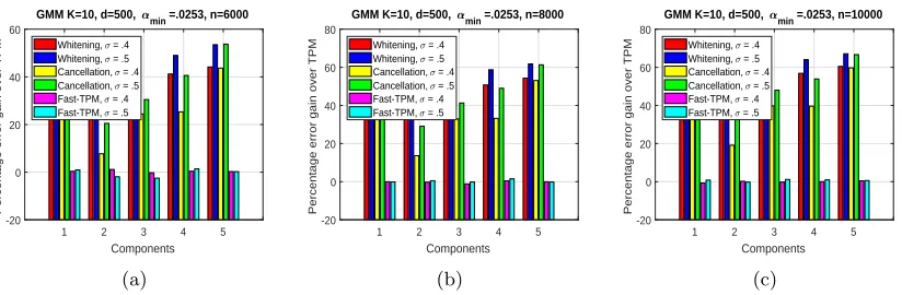
Gaussian mixture model: We generate synthetic data sets for GMM with differentk, d, αi, σ,andv.Figure 1 shows the percentage relative error gains of the Whitening,

Cancel-lation, and Fast-TPM algorithms over the TPM algorithm in a GMM with various values of k, d, αi, σ, andn. Theµiwere generated randomly over the sphere of normr= 10.We define

αmin := miniαi.The side information vectorv was chosen as follows. Let{v1, . . . , vk}be a

(16)

GMM K=10, d=500, _min =.0253, n=6000

1 2 3 4 5

Components -20

0 20 40 60

Percentage error gain over TPM

Whitening, = .4 Whitening, = .5 Cancellation, = .4 Cancellation, = .5 Fast-TPM, = .4 Fast-TPM, = .5

(a)

GMM K=10, d=500, _min =.0253, n=8000

1 2 3 4 5

Components -20

0 20 40 60 80

(b)

GMM K=10, d=500, _min =.0253, n=10000

1 2 3 4 5

Components -20

0 20 40 60 80

(c)

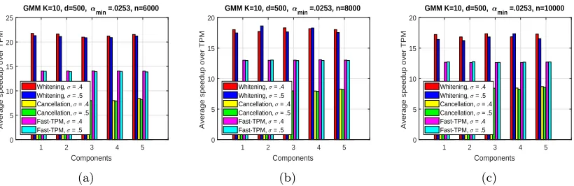
Figure 1: Figure showing the percentage relative error gain by the Whitening, Cancellation, and Fast-TPM algorithm over the TPM algorithm for 5 components of increasing size, in a GMM with k = 10, d = 500, σ ∈ {.4, .5}, and three different sample complexities (a) n = 6000 (b) n = 8000 (c) n = 10000. Our algorithms shows increasingly better gain over TPM and Fast-TPM asαi, σ and nincrease.

choose v = √γv1+ p

(1−γ)/(k−1)Pk

i=2vi for some γ ∈ (0,1) such that the condition

hµ1, vi>hµi, viis satisfied. We observe that in all the cases, our algorithms have lower error

(positive error gain) than both the tensor algorithms. Moreover, our methods’ advantage increases with increasing proportion αi, increasing sample size n, and increasing variance

σ.We also observe that the Fast-TPM algorithm has the same error performance as TPM (error gain close to zero).

Figure 2 gives an example where the Whitening algorithm can successfully recover even rare components. Here we consider a GMM withk= 10, d= 500 with the rarest component having probability αmin =.0037. Again we observe positive relative error gains over TPM

algorithm for increasing number of samplesn.

In Figure 3 we plot the speedup of the algorithms over TPM, and observe that the Whitening and Cancellation algorithms are much faster (high speedup) than the TPM algorithm. We also observe that the Fast-TPM algorithm is faster than TPM and Cancella-tion algorithms, but slower than Whitening algorithm. Note that, while it is also possible to speed up the basic TPM algorithm compared here using techniques such as randomized svd and stochastic tensor gradient descent [Huang et al. 2015], such approximate methods will reduce the overall accuracy. Moreover the randomized svd techniques can also be applied to the search algorithms presented in this paper, to obtain further speedups.

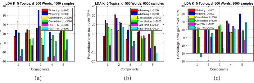
Topic Modeling: We generate a synthetic LDA document corpus according to the model in Blei et al. (2003). The lengths of the documents are generated using a Poission(L) distribution where L is the mean document length. In Figure 4 we plot the percentage relative error gain of the Whitening, Cancellation, and Fast-TPM algorithms over the TPM algorithm. Our side information was a labeled wordw satisfying µ1(w)> µi(w) for i6= 1.

(17)

GMM K=10, d=500, _min = .0037, 5000 samples

1 2 3 4 5 6 7 8 9 10 Components 0 10 20 30 40 50 60

= .3 = .4 = .5 = .6

(a)

1 2 3 4 5 6 7 8 9 10 Components 0 10 20 30 40 50 60 70

= .3 = .4 = .5 = .6

(b)

1 2 3 4 5 6 7 8 9 10 Components 0 10 20 30 40 50 60 70

= .3 = .4 = .5 = .6

(c)

Figure 2: Figure showing the percentage relative error gain of the Whitening algorithm over the TPM algorithm in presence of rare components (αmin = .0037), for

a GMM with k = 10, d = 500, σ ∈ {.3, .4, .5, .6}, and number of samples (a) n= 5000 (b)n= 6000 (c)n= 8000.The Whitening algorithm recovers even the rarest component with increasing error gain over TPM as the number of samples increase.

GMM K=10, d=500, _min =.0253, n=6000

1 2 3 4 5

Components 0 5 10 15 20 25

Average speedup over TPM

(a)

GMM K=10, d=500, _min =.0253, n=8000

1 2 3 4 5

Components 0 5 10 15 20

(b)

GMM K=10, d=500, _min =.0253, n=10000

1 2 3 4 5

Components 0 5 10 15 20

(c)

Figure 3: Figure showing the average speedup of Whitening, Cancellation, and Fast-TPM algorithms over TPM, for 5 components of increasing size, in a GMM with k= 10, d= 500, σ∈ {.4, .5},and three different sample complexities (a)n= 6000 (b) n= 8000 (c) n= 10000.The Whitening algorithm is the fastest.

algorithm still outperforms it. Note that the performance varies across topics since the probability of the labeled word is different for each topic.

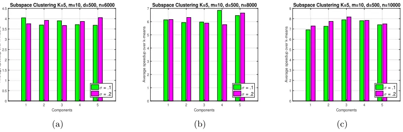
Subspace Clustering: We generate synthetic data for the subspace clustering model described in section 3.4 using parameters d = 500, k = 5, m = 10, and αi ∈ [.1, .3]. First

(18)

LDA K=5 Topics, d=500 Words, 4000 samples

1 2 3 4 5

Components -20

-10 0 10 20 30 40

Whitening, L=2000 Whitening, L=3000 Cancellation, L=2000 Cancellation, L=3000 Fast-TPM, L=2000 Fast-TPM, L=3000

(a)

1 2 3 4 5

Components -20

-10 0 10 20 30 40

(b)

1 2 3 4 5

Components -30

-20 -10 0 10 20 30 40

(c)

Figure 4: Figure showing the percentage relative error gain in each component of the Whitening, Cancellation, and Fast-TPM algorithms over the TPM algorithm in an LDA model with k = 5, d = 500, mean document length L ∈ {2000,3000}, and number of documents (a)n= 4000 (b) n= 6000 (c) n= 8000.The Whiten-ing algorithm show an improvement over TPM and Fast-TPM with increasWhiten-ing samples.

to it. Traditional subspace clustering algorithms, which assume points to lie exactly on the subspace, may not perform well. The TPM algorithm is also not well suited for this model since (a) the required moment tensor will be of 4th_{order resulting in high computation cost}

(b) even if mk basis of the tensor are recovered, finding the target subspace will involve a further combinatorial search of mk_m

subspaces and finding the one having the strongest projection of v. Therefore we choose the k-means algorithm as our baseline for this model and compare with Algorithm 3. First we compute k clusters using k-means, then we find an mdimensional basis for each cluster using svd, finally we choose the target subspace as the one having the largest projection ofv. IfUb₁ is the estimated orthonormal basis for the target subspace U1,we compute the error as E=kUb₁Ub₁T −U₁U₁Tk/kU₁U₁Tk.

Figure 5 shows that Algorithm 3 has a much better error performance over k-means. In the speedup plots in Figure 6 we also observe that our subspace search algorithm is over 4X times faster than k-means.

4.2 Real Data Sets

Topic Modeling: In this section we compare the performance of Whitening algorithm with a recent non-negative matrix factorization based topic modeling algorithm by Arora et al. (2013) (we refer this as NMF algorithm), and also the semi-supervised version of this NMF algorithm (we refer to this as SS-NMF). We test on two real large data sets; (a) New York Times news article data set [UCI 2008] (300,000 articles) (b) Yelp data set of business reviews [Yelp 2014] (335,022 reviews). We run both algorithms for k = 100 topics. For this experiment we do not consider the TPM algorithm by Anandkumar et al. (2014) since its runtime with k= 100 topics becomes extremely large on these data sets.1

1. To be more precise, with justk= 10 topics, the tensor algorithm takes 908 seconds in NY Times data

(19)

Subspace Clustering K=5, m=10, d=500, n=6000

1 2 3 4 5

Components 0 20 40 60 80 100

Percentage error gain over k-means

= .1 = .2

(a)

1 2 3 4 5

Components 0 20 40 60 80 100

= .1 = .2

(b)

1 2 3 4 5

Components 0 20 40 60 80 100

= .1 = .2

(c)

Figure 5: Figure showing the percentage relative error gain by our subspace search al-gorithm (Alal-gorithm 3) over k-means for 5 components of increasing size, in a subspace clustering model with k = 5, m = 10, d = 500, σ ∈ {.1, .2}, and three different sample complexities (a) n = 6000 (b) n = 8000 (c) n = 10000. Our algorithm shows much better error performance than k-means.

1 2 3 4 5

Components 0 0.5 1 1.5 2 2.5 3 3.5 4 4.5

Average speedup over k-means

σ = .1

σ = .2

(a)

1 2 3 4 5

Components 0 1 2 3 4 5 6 7

σ = .1 σ = .2

(b)

1 2 3 4 5

Components 0 1 2 3 4 5 6 7 8 9

σ = .1

σ = .2

(c)

Figure 6: Figure showing the average speedup of our subspace search algorithm (Algorithm 3) over k-means, for 5 components of increasing size, in a subspace clustering model with k = 5, m = 10, d = 500, σ ∈ {.1, .2}, and three different sample complexities (a)n= 6000 (b) n= 8000 (c) n= 10000. Our subspace clustering algorithm shows high speedup over k-means.

In contrast, the NMF algorithm is known to be faster, and produce topics of comparable quality to more popular variational inference based algorithms [Blei et al. 2003]. The side information for this experiment are chosen as follows. First from the set of topics produced by NMF algorithm we choose a subset of interpretable topics, then we choose labeled words representative of these topics. We test with a set of 62 labeled words for NY Times data set and 54 labeled words for Yelp data set. Note that given labeled word wl

(20)

the weighted word-word co-occurrence matrixQw where we re-weigh each document by the

normalized frequency of the labeled word wl. Then we apply the NMF algorithm [Arora

et al. 2013] on this weighted matrix Qw.All three algorithms were implemented in Python.

Performance metric: We compare the quality of the topics returned by Whitening, NMF,

and SS-NMF algorithms using the pointwise mutual information (PMI) score, known to be a good metric for topic coherence [Newman et al. 2010; R¨oder et al. 2015]. However in order to also capture the relevance of the estimated topic to the labeled word we compute PMI score for topicias,

P M I(topic i) = 1 20

X

w∈Ti

20

log p(wl, w) p(wl)p(w)

where wl is the labeled word, T20i is the set of top 20 words in the i-th topic. The probabilitiesp(wl, w), p(w), p(wl) are computed over a larger data set of English Wikipedia

articles to reduce noise [Newman et al. 2011]. For whitening algorithm we chooseα0=.01. Note that other supervised topic modeling algorithms e.g. supervised LDA by Mcauliffe and Blei (2008), labeled LDA by Ramage et al. (2009) require a much stronger notion of side-information than just labeled words, hence we could not compare with them.

(a) (b)

Figure 7: Figure comparing the performance of Whitening, NMF [Arora et al. 2013], and semi-supervised NMF (SS-NMF) algorithms on NY Times and Yelp data sets. (a) Topics estimated by Whitening algorithm have the best PMI score in 40 out of 62 labeled words for NY Times data set, and 35 out of 54 labeled words in Yelp data set. (b) Whitening shows more than 2X speedup over competing algorithm in both data sets.

In Figure 7 (a) we plot the percentage of labeled words for which each algorithm has the best PMI score. Observe that for most labeled words (40 out of 62 labeled words for NY Times data set, and 35 out of 54 labeled words in Yelp data set) the Whitening algorithm estimates topic with better PMI score over NMF and SS-NMF algorithms. The Whitening algorithm is also more than twice as fast as NMF and SS-NMF2 as shown in Figure 7 (b).

(21)

A complete list of topics and PMI scores returned by the algorithms for every labeled word is presented in Tables 2, 3 of Appendix B. Notice that the Whitening algorithm often esti-mates more coherent topics which are more relevant to the given labeled word than topics produced by the NMF/SS-NMF algorithm. For example in NY Times data set with the labeled word student the Whitening algorithm returns top five words in the topic as

stu-dent, school, teacher, percent, program; however those returned by NMF algorithm aretest,

school, student, ignore, export; and those by SS-NMF algorithm are student, university,

shooting, shot, rampage.

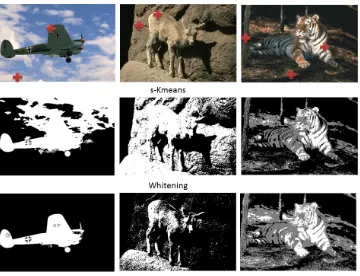
Parallel image segmentation: One method to perform image segmentation is to use GMM clustering. In this experiment we demonstrate how GMM search algorithm can be used to parallelize image segmentation in vision applications. For this we consider the BSDS500 data set introduced in Arbelaez et al. (2011) and choose a subset of 70 images having less than 4 segments in the ground truth. Note that this data set has up to six ground truth segmentation by human users for each image. We randomly choose one pixel from each segment in ground truth as side-informationv. We compare our Whitening algorithm with the seeded k-means clustering [Basu et al. 2002] where the centers are initialized by these side-information pixels (we refer to this as s-Kmeans). The Whitening algorithm uses one pixel from the i-th cluster to compute µi, in parallel for every i, and then it assigns

each pixel to its closestµi.The segmentation quality is compared using normalized mutual

information (NMI) metric [Manning et al. 2008]. To avoid local minimum in s-Kmeans we consider the maximum NMI over 5 initializations of side-information for each ground truth, and then we compute average NMI over all ground truths for an image.

Figure 8: Figure comparing the performance of image segmentation by Whitening (row 3) and s-Kmeans (row 2) algorithms, with images selected from the BSDS500 data set. The side-information pixels are shown in red plus in the original image (row 1). In the segmented images (rows 2,3) the segments are shown in differ-ent shades. Observe that the Whitening algorithm often isolates the foreground segment better than s-Kmeans.

(22)

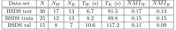
Data set N NW NK TW (s) TK (s) N M IW N M IK

BSDS test 30 17 13 6.7 81.5 0.17 0.13 BSDS train 25 12 13 8.2 89.8 0.15 0.15 BSDS val 15 8 7 10.6 117.2 0.11 0.09

Table 1: Table comparing the performance of Whitening and s-Kmeans algorithm on BSDS data set. N is the total number of images, NW is the number of images where

segmentation produced by Whitening has a better NMI than s-Kmeans, and NK

is the number of images where segmentation of s-Kmeans has a better NMI. TW

is the median runtime of Whitening algorithm and TK is the median runtime of

s-Kmeans. N M IW andN M IK are the median NMI scores for the Whitening and

s-Kmeans algorithms respectively. Whitening runs much faster than s-Kmeans.

in BSDS train and BSDS val data sets. However the Whitening algorithm runs an order of magnitude faster than s-Kmeans.

5. Conclusion and Discussion

In this paper we developed a new, simple and flexible framework for incorporating side information into mixture model learning. The underlying motivation was to provide a principled way to take into account extra input (e.g. generated by human data analysts etc.). Even for cases where this input is very limited compared to the size/dimensionality of the data, we show meaningful statistical and computational performance improvement over baseline unsupervised and semi-supervised methods. More generally, developing methods which work with very limited human input is a promising research endeavor, in our opinion.

Acknowledgments

(23)

Appendix A. More Experiments for Gaussian Mixture Models

In Figure 9 we show the sensitivity of the Whitening and Cancellation algorithms in GMM withk= 20, d= 500,all equal probability components, and two different values ofσ andn. Observe that the percentage error gain of the algorithms decreases with decreasing values of δ = mini6=1h_hµ1,v_µ_i_,v_ii, as we would expect, and it eventually becomes negative when the performance become worse than TPM algorithm. Also here the Cancellation algorithm shows lesser sensitivity, hence better performance compared to the Whitening algorithm.

GMM K=20, d=500, =.05 (all equal), n=6000

Inf 5.62 3.97 3.23 2.77 2.44 2.20

-40 -20 0 20 40

Whitening, = .5 Whitening, = .6 Cancellation, = .5 Cancellation, = .6

(a)

GMM K=20, d=500, =.05 (all equal), n=8000

Inf 5.62 3.97 3.23 2.77 2.44 2.20

-50 0 50

Whitening, = .5 Whitening, = .6 Cancellation, = .5 Cancellation, = .6

(b)

Figure 9: Sensitivity plots showing how the percentage relative error gain of the Whitening and Cancellation algorithms over the TPM algorithm decrease with decreasing values of the parameter δ = mini6=1h_hµ1,v_µ_i_,vi_i, in GMM with k = 20, d = 500, all equal probability components, for different values of variance σ ∈ {.5, .6}, and two different sample complexities (a)n= 6000 (b)n= 8000.

Appendix B. Complete Results on New York Times and Yelp Data Set

In this section we provide more detailed result of our experiments on NY Times and Yelp data sets. In Tables 2, 3 we show for every labeled word, the top five words in the topics computed by Whtening, NMF, and SS-NMF algorithms along with their corresponding PMI scores.

Table 2: Results of topic search by Whitening and NMF

algo-rithms on NYtimes data set of 300,000 news articles using K = 100 topics and 62 labeled words.

NY Times data set Label

word

Algo topword-1 topword-2 topword-3 topword-4 topword-5 PMI

passenger

Whitening flight security passenger airport hour 0.1424

NMF security government official percent bill 0.0499

SSNMF passenger plane flight fire crash 0.1711

coach

(24)

Label word

NMF team coach season player jet 0.1740

SSNMF coach arrived assistant defenseman ended 0.1756

art

Whitening information question today eastern daily 0.0255

NMF art show dessert book home 0.0769

SSNMF art artist show painting museum 0.1250

campaign

Whitening campaign al gore money political republican 0.1530

NMF al gore campaign george bush president bush 0.1608

SSNMF nra florida article senator presidential 0.0926

energy

Whitening corp meeting list dividend partial 0.0815

NMF corp meeting list group dividend 0.0570

SSNMF partial energy dividend meeting corp 0.0254

tax

Whitening tax cut taxes percent income 0.2126

NMF graf president bush mail information 0.0722

SSNMF tax income cut taxes site 0.2279

chef

Whitening cup minutes food article add 0.0227

NMF buy panelist flavor thought product 0.0130

SSNMF tobacco chef restaurant pastry article 0.1495

oil

Whitening oil cup minutes prices companies 0.1460

NMF oil million prices percent market 0.0928

SSNMF oil company listing largest brazil 0.0902

court

Whitening court case law decision lawyer 0.2288

NMF official court case attack government 0.1285

SSNMF chicago court decision ruling justices 0.1834

election

Whitening election ballot vote voter florida 0.2132

NMF election ballot al gore bush vote 0.2155

SSNMF gained election article presidential independence 0.1702

lawyer

Whitening case court lawyer death trial 0.1830

SSNMF lawyer rat legal client jokes 0.1314

anthrax

Whitening mail official anthrax attack worker 0.0600

NMF anthrax official mail worker letter 0.0156

SSNMF anthrax poverty cb show return -0.0776

golf

Whitening tiger wood shot round player tour 0.1288

NMF tiger wood shot round player play 0.1356

SSNMF misstated master tee hit golf 0.1356

bacteria

Whitening mail anthrax official test found -0.0763

NMF anthrax official mail worker letter -0.1097

SSNMF mas bacteria con una anos -0.2420

film

Whitening film movie director character actor 0.1906

NMF article misstated new york company million 0.0288

SSNMF kiss film actress article role 0.1295

tourist

Whitening million www percent building night 0.0481

NMF team tour lance

arm-strong

won race -0.0405

SSNMF tourist million visitor official campaign 0.0995

horse

Whitening race won win run track 0.1129

NMF race won horse win kentucky

derby

0.1338

SSNMF horse truck road official killed 0.0433

republican

Whitening campaign george bush bush election republican 0.2449

SSNMF republican democrat democratic house parties 0.1053

computer

(25)

Label word

NMF company computer microsoft system companies 0.1533

SSNMF computer chip mail program buy 0.1903

palestinian

Whitening palestinian israel israeli yasser

arafat

peace 0.2189

NMF palestinian israel official israeli yasser arafat 0.1950

SSNMF palestinian reformer reform authority arab 0.1519

movie

Whitening film movie director character actor 0.1492

NMF film show actor movie thought 0.0901

SSNMF red sox movie interview seattle host 0.0388

tennis

Whitening player play won game women 0.1054

NMF game play player point andre agassi 0.1187

SSNMF motif tennis season pros image 0.1480

fight

Whitening won night fight win sport 0.0566

NMF fight mike tyson lennox lewis million round 0.1181

SSNMF fight pound fighter beat boxing 0.1254

music

Whitening music song record album band 0.2298

NMF music company million companies napster 0.0812

SSNMF music mp3 customer digital online 0.0150

tablespoon

Whitening cup minutes add oil tablespoon 0.0608

NMF cup minutes add tablespoon water 0.0431

SSNMF coffee bean tablespoon cup ground -0.0765

nuclear

Whitening bush US official system administration 0.1223

NMF official bush government US nuclear 0.1356

SSNMF ibm nuclear computer research fastest -0.0253

racing

Whitening race car driver team season 0.1443

NMF car race driver team season 0.1319

SSNMF sport file los angeles racing notebook -0.0640

war

Whitening military taliban war afghanistan us 0.0916

NMF taliban official afghanistan government us 0.0796

SSNMF russian war chechnya army veteran 0.1296

quarterback

Whitening yard season game play team 0.2389

NMF game team play yard season 0.1773

SSNMF effort quarterback ucla heroic alabama 0.1472

stock

Whitening stock market percent company fund 0.1585

NMF percent stock market company companies 0.1338

SSNMF stock market price shares investment 0.0507

ball

Whitening game run yard play hit 0.1782

NMF run game inning hit season 0.1361

SSNMF ball hit run inning home 0.1708

patient

Whitening patient doctor care health drug 0.2532

NMF official virus percent new york found 0.1003

SSNMF patient study doctor article brain 0.1334

champion

Whitening won win round shot tiger wood 0.1029

NMF fight mike tyson lennox lewis million round 0.0955

SSNMF olympic champion final meet medalist 0.1177

business

Whitening business company question information companies 0.0887

NMF information eastern commentary daily business 0.0311

SSNMF publication business send released businesses 0.0996

government

Whitening government official country federal political 0.1524

SSNMF program government computer local newspaper 0.0784

season

Whitening season team game games play 0.1799

(26)

Label word

SSNMF season cotton fact simple variety 0.0626

prison

Whitening death case lawyer court trial 0.1333

NMF advise spot earlier held today -0.0340

SSNMF prison inmates security population bed 0.1472

internet

Whitening file spot internet read output 0.0359

NMF file spot new york sport los angeles 0.0228

SSNMF wonderful mail al gore george bush message 0.0766

rain

Whitening air part high wind rain 0.1963

NMF air wind shower rain storm 0.1939

SSNMF chicago sun

times

nominated rain east thought 0.0179

game

Whitening game team play games season 0.2000

NMF team game season play games 0.1722

SSNMF covering game tonight coverage celebration 0.0531

voter

Whitening election ballot vote percent voter 0.2068

NMF election ballot al gore bush vote 0.1870

SSNMF voter poll percent primary election 0.2067

baseball

Whitening player team season game sport 0.1691

NMF team chicago

white sox

mariner season player 0.1803

SSNMF velocity baseball air shot test 0.0629

student

Whitening student school teacher percent program 0.2077

NMF test school student ignore export 0.0729

SSNMF student university shooting shot rampage 0.1396

president

Whitening president vice white house george bush executive 0.2116

SSNMF hedge president television broadway produced 0.0226

afghan

Whitening taliban afghanistan military us war 0.1684

NMF taliban official afghanistan government us 0.1413

SSNMF afghan afghanistan blanket friend country 0.0577

medal

Whitening team games won women american 0.1822

NMF team tour lance

arm-strong

won race 0.0348

SSNMF endit medal honor winner newspaper 0.0786

teacher

Whitening school student teacher high program 0.1566

NMF test school student ignore export 0.0388

SSNMF teacher program pay school teaching 0.1499

television

Whitening show home network television night 0.1721

NMF los angeles

daily new

spot newspaper new york show 0.1456

SSNMF clinton home television survived tonight -0.0090

democratic

Whitening al gore campaign election political republican 0.1837

SSNMF environmental democratic national

committee

nominee fund 0.0813

onion

Whitening cup minutes add oil tablespoon 0.1039

NMF cup minutes add tablespoon water 0.1072

SSNMF flavor panelist ounces buy onion 0.1188

campus

Whitening student school college teacher program 0.1314

NMF game season team play coach -0.0595

SSNMF campus operation aol building center 0.0645

car

Whitening car driver race racing seat 0.2047

(27)

Label word

SSNMF car team race driver winston cup 0.1516

industry

Whitening companies percent company business industry 0.1430

NMF music company million companies napster 0.0821

SSNMF xxx show trade software entertainment 0.1161

planet

Whitening film today system movie team -0.0054

NMF wire inadvertently kill mandatory today -0.0750

SSNMF captor planet film kill astronomer 0.0949

credit

Whitening bill money member system number 0.1257

NMF bill tax bush member percent 0.0287

SSNMF donation card credit account voted 0.1382

race

Whitening race car driver won win 0.1917

NMF car race driver team season 0.1814

SSNMF amazing race show tonight sit 0.0502

wine

Whitening cup minutes food add oil 0.0499

NMF wine wines percent company million 0.0748

SSNMF wine wines bottle bottles age 0.1082

prosecutor

Whitening case death lawyer court trial 0.1952

SSNMF prosecutor lawyer attorney incorrectly general 0.1406

team

Whitening team season game player play 0.1654

NMF team game season play games 0.1558

SSNMF team qualify olympic article member 0.1530

economy

Whitening percent market economy stock cut 0.1528

NMF percent stock market company companies 0.1048

SSNMF percent economy quarter rate recession 0.1452

wind

Whitening air high part wind rain 0.1909

NMF air wind shower rain storm 0.1895

SSNMF wash wind school winter white 0.1902

software

Whitening microsoft computer system company software 0.1981

NMF company computer microsoft system companies 0.1911

SSNMF xxx software industry show trade 0.1222

Table 3: Results of topic search by Whitening and NMF

al-gorithms on Yelp data set of 335,022 reviews of businesses using K = 100 topics and 54 labeled words.

Yelp data set Label

word

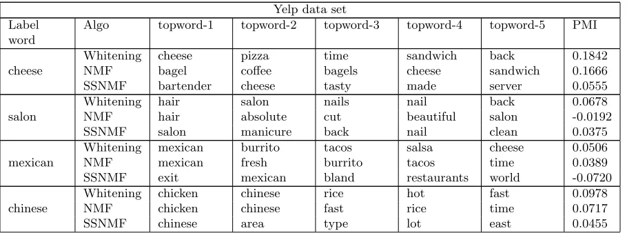
cheese

Whitening cheese pizza time sandwich back 0.1842

NMF bagel coffee bagels cheese sandwich 0.1666

SSNMF bartender cheese tasty made server 0.0555

salon

Whitening hair salon nails nail back 0.0678

NMF hair absolute cut beautiful salon -0.0192

SSNMF salon manicure back nail clean 0.0375

mexican

Whitening mexican burrito tacos salsa cheese 0.0506

NMF mexican fresh burrito tacos time 0.0389

SSNMF exit mexican bland restaurants world -0.0720

chinese

Whitening chicken chinese rice hot fast 0.0978

NMF chicken chinese fast rice time 0.0717