Non-linear Causal Inference using Gaussianity Measures
Daniel Hern´andez-Lobato [email protected]
Universidad Aut´onoma de Madrid Calle Francisco Tom´as y Valiente 11, Madrid 28049, Spain
Pablo Morales-Mombiela [email protected]
Quantitative Risk Research Calle Faraday 7,
Madrid 28049, Spain
David Lopez-Paz∗ [email protected]
Facebook AI Research 6 rue Menars, Paris 75002, France
Alberto Su´arez [email protected]
Universidad Aut´onoma de Madrid Calle Francisco Tom´as y Valiente 11, Madrid 28049, Spain
Editor:Isabelle Guyon and Alexander Statnikov
Abstract
We provide theoretical and empirical evidence for a type of asymmetry between causes and effects that is present when these are related via linear models contaminated with additive non-Gaussian noise. Assuming that the causes and the effects have the same distribution, we show that the distribution of the residuals of a linear fit in the anti-causal direction is closer to a Gaussian than the distribution of the residuals in the causal direction. This Gaussianization effect is characterized by reduction of the magnitude of the high-order cumulants and by an increment of the differential entropy of the residuals. The problem of non-linear causal inference is addressed by performing an embedding in an expanded feature space, in which the relation between causes and effects can be assumed to be linear. The effectiveness of a method to discriminate between causes and effects based on this type of asymmetry is illustrated in a variety of experiments using different measures of Gaussianity. The proposed method is shown to be competitive with state-of-the-art techniques for causal inference.
Keywords: causal inference, Gaussianity of the residuals, cause-effect pairs
1. Introduction
The inference of causal relationships from data is one of the current areas of interest in the artificial intelligence community,e.g. (Chen et al., 2014; Janzing et al., 2012; Morales-Mombiela et al., 2013). The reason for this surge of interest is that discovering the causal
structure of a complex system provides an explicit description of the mechanisms that generate the data, and allows us to understand the consequences of interventions in the system (Pearl, 2000). More precisely, automatic causal inference can be used to determine how modifications of the value of certain relevant variables (the causes) influence the values of other related variables (the effects). Therefore, understanding cause-effect relations is of paramount importance to control the behavior of complex systems and has applications in industrial processes, medicine, genetics, economics, social sciences or meteorology.
Causal relations can be determined in complex systems in three different ways. First, they can be inferred from domain knowledge provided by an expert, and incorporated in an ad-hoc manner in the description of the system. Second, they can be discovered by performing interventions in the system. These are controlled experiments in which one or several variables of the system are forced to take particular values. Interventions constitute a primary tool for identifying causal relationships. However, in many situations they are unethical, expensive, or technically infeasible. Third, they can be estimated using causal discovery algorithms that use as input purely uncontrolled and static data.
This last approach for causal discovery has recently received much attention from the machine learning community (Shimizu et al., 2006; Hoyer et al., 2009; Zhang and Hyv¨arinen, 2009). These methods assume a particular model for the mapping mechanisms that link causes to effects. By specifying particular conditions on the mapping mechanism and the distributions of the cause and noise variables, the causal direction becomes identifiable Chen et al. (2014). For instance, Hoyer et al. (2009) assume that the effect is a non-linear transformation of the cause plus some independent additive noise. A potential drawback of these methods is that the assumptions made by the particular model considered could be unrealistic for the data under study.
In this paper we propose a general method for causal inference that belongs to the third of the categories described above. Specifically, we assume that the cause and the effect variables have the same distribution and are linked by a linear relationship contaminated with non-Gaussian noise. For the univariate case we prove that, under these assumptions, the magnitude of the cumulants of the residuals of order higher than two is smaller for the linear fit in the anti-causal direction than in the causal one. Since the Gaussian is the only distribution whose cumulants of order higher than 2 are zero, statistical tests based on measures of Gaussianity can be used for causal inference. An antecedent of this result is the observation that, when cause and effect have the same distribution, the residuals of a fit in the anti-causal direction have higher entropy than in the causal direction (Hyv¨arinen and Smith, 2013; Kpotufe et al., 2014). Since the residuals of the causal and anti-causal linear models have the same variance and the Gaussian is the distribution that maximizes the entropy for a fixed variance, this means that the distribution of the latter is more Gaussian than the former.
The problem of non-linear causal inference is addressed by embedding the original prob-lem in an expanded feature space. We then make the assumption that the non-linear relation between causes and effects in the original space is linear in the expanded feature space. The computations required to make inference on the causal direction based on this embedding can be readily carried out using kernel methods.
In summary, the proposed method for causal inference proceeds by first making a trans-formation of the original variables so that causes and effects have the same distribution. Then we perform kernel ridge regression in both the causal and the anti-causal directions. The dependence between causes and effects, which is non-linear in the original space, is assumed to be linear in the kernel-induced feature space. A statistical test is then used to quantify the degree of similarity between the distributions of these residuals and a Gaussian distribution with the same variance. Finally, the direction in which the residuals are less Gaussian is identified as the causal one.
The performance of this method is evaluated in both synthetic and real-world cause-effect pairs. From the results obtained it is apparent that the anti-causal residuals of a linear fit in the expanded feature space are more Gaussian than the causal residuals. In general, it is difficult to estimate the entropy from a finite sample (Beirlant et al., 1997). Empirical estimators of high order cumulants involve high order moments, which means they often have large variance. As an alternative, we propose to use statistical tests based on theenergy distance to characterize the Gaussianization effect for the residuals of linear fits in the causal and anti-causal directions. Tests based on the energy distance were analyzed in depth by Sz´ekely and Rizzo (2005). They have been shown to be related to homogeneity tests based on embeddings in a Reproducing Kernel Hilbert Space (Gretton et al., 2012). An advantage of energy distance-based statistics is that they can be readily estimated from a sample by computing expectations of pairwise Euclidean distances. The energy distance generally provides better results than the entropy or cumulant-based Gaussianity measures. In the problems investigated, the accuracy of the proposed method, using the energy distance to the Gaussian, is comparable to other state-of-the-art techniques for causal discovery.
The rest of the paper is organized as follows: Section 2 illustrates that, under certain conditions, the residuals of a linear regression fit are closer to a Gaussian in the anti-causal direction than in the causal one, based on a reduction of the high-order cumulants and on an increment of the entropy. This section considers both the univariate and multivariate cases. Section 3 adopts a kernel approach to carry out a feature expansion that can be used to detect non-linear causal relationships. We also show here how to compute the residuals in the expanded feature space, and how to choose the different hyper-parameters of the proposed method. Section 4 contains a detailed description of the implementation. In section 6 we present the results of an empirical assessment of the proposed method in both synthetic and real-world cause-effect data pairs. Finally, Section 7 summarizes the conclusions and puts forth some ideas for future research.
2. Asymmetry Based on the Non-Gaussianity of the Residuals of Linear Models
alternativelyY causesX,i.e.,Y → X. For this purpose, we exploit an asymmetry between causes an effects. This type of asymmetry can be uncovered using statistical tests that measure the non-Gaussianity of the residuals of linear regression models obtained from fits in the causal and in the anti-causal direction.
To motivate the methodology that we have developed, we will proceed in stepwise man-ner. First we analyze a special case in one dimension: We assume that X and Y have the same distribution and are related via a linear model contaminated with additive i.i.d. non-Gaussian noise. The noise is independent of the cause. Under these assumptions we show that the distribution of the residuals of a linear fit in the incorrect (anti-causal) direc-tion is closer to a Gaussian distribudirec-tion than the distribudirec-tion of the residuals in the correct (causal) direction. For this, we use an argument based on the reduction of the magnitude of the cumulants of order higher than 2. The cumulants are defined as the derivatives of the logarithm of the moment-generating function evaluated at zero (Cornish and Fisher, 1938; McCullagh, 1987).
The Gaussianization effect can be characterized also in terms of an increase of the entropy. The proof is based on the results of Hyv¨arinen and Smith (2013), which are extended in this paper to the multivariate case. In particular, we show that the entropy of the residuals of a linear fit in the anti-causal direction is larger or equal than the entropy of the residuals of a linear fit in the causal direction. Since the Gaussian it the distribution that has maximum entropy, given a particular covariance matrix, an increase of the entropy of the residuals means that their distribution becomes closer to the Gaussian.
Finally, we note that it is easy to guarantee that X and Y have the same distribution in the case that these variables are unidimensional and continuous. To this end we only have to transform one of the variables (typically the cause random variable) using the probability integral transform, as described in Section 4. However, after the data have been transformed, the relation between the variables will no longer be linear in general. Thus, to address non-linear cause-effect problems involving univariate random variables the linear model is formulated in an expanded feature space, where the multivariate analysis of the Gaussianization effect is also applicable. In this feature space all the computations required for causal inference can be formulated in terms of kernels. This can be used to detect non-linear causal relations in the original input space and allows for an efficient implementation of the method. The only assumption is that the non-linear relation in the original input space is linear in the expanded feature space induced by the selected kernel.
2.1 Analysis of the Univariate Case Based on Cumulants
LetX andYbe one-dimensional random variables that have the same distribution. Without further loss of generality, we will assume that they have zero mean and unit variance. Let
x= (x1, . . . , xN)T and y= (y1, . . . , yN)T beN paired samples drawn i.i.d. fromP(X,Y).
Assume that the causal direction is X → Y and that the measurements are related by a linear model
yi =wxi+i, i⊥xi, ∀i , (1)
A linear model in the opposite direction,i.e.,Y → X, can be built using least squares
xi =wyi+ ˜i, (2)
wherew= corr(Y,X) is the same coefficient as in the previous model. The residuals of this reversed linear model are defined as ˜i =xi−wyi.
Following an argument similar to that of Hern´andez-Lobato et al. (2011) we show that the residuals {˜i}Ni=1 in the anti-causal direction are more Gaussian than the residuals {i}Ni=1 in the actual causal direction X → Y based on a reduction of the magnitude of
the cumulants. The proof is based on establishing a relation between the cumulants of the distribution of the residuals in both the causal and the anti-causal direction. First, we show that κn(yi), the n-th order cumulant of Y, can be expressed in terms of κn(i), the n-th
order cumulant of the residuals:
κn(yi) =wnκn(xi) +κn(i) =wnκn(yi) +κn(i) =
1
1−wnκn(i). (3)
To derive this relation we have used (1), that xi and yi have the same distribution (and
hence have the same cumulants), and standard properties of cumulants (Cornish and Fisher, 1938; McCullagh, 1987). Furthermore,
κn(˜i) =κn(xi−wyi) =κn(xi−w2xi−wi) = (1−w2)nκn(xi) + (−w)nκn(i)
= (1−w2)nκn(yi) + (−w)nκn(i) =
(1−w2)n
1−wn κn(i) + (−w) nκ
n(i)
=cn(w)κn(i), (4)
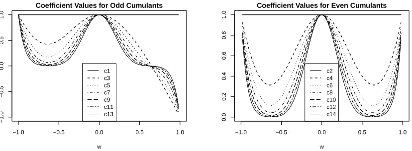
where we have used the definition of ˜i and (3) In Figure 1 the value of
cn(w) =
(1−w2)n
1−wn + (−w)
n. (5)
is displayed as a function of w ∈ [−1,1]. Note that c1(w) = c2(w) = 1 independently of
the value of w. This means that the mean and the variance of the residuals are the same in both the causal and anti-causal directions. For n > 2, |cn(w)| ≤ 1 with equality only
for w = 0 and w = ±1. The result is that the high-order cumulants of the residuals in the anti-causal direction are smaller in magnitude that the corresponding cumulants in the causal direction. Using the observation that all the cumulants of the Gaussian distribution of order higher than two are zero (Marcinkiewicz, 1938), we conclude that the distribution of the residuals in the anti-causal direction is closer to the Gaussian distribution than in the causal direction.
In summary, we can infer the causal direction by (i) fitting a linear model in each possible direction, i.e.,X → Y and Y → X, and (ii) carrying out statistical tests to detect the level of Gaussianity of the two corresponding residuals. The direction in which the residuals are less Gaussian is expected to be the correct one.
2.2 Analysis of the Multivariate Case Based on Cumulants
● ●
−1.0 −0.5 0.0 0.5 1.0
−1.0
−0.5
0.0
0.5
1.0
Coefficient Values for Odd Cumulants
w c1 c3 c5 c7 c9 c11 c13
−1.0 −0.5 0.0 0.5 1.0
0.0
0.2
0.4
0.6
0.8
1.0
Coefficient Values for Even Cumulants
w c2 c4 c6 c8 c10 c12 c14
Figure 1: Values of the functioncn(·) as a function of w for each cumulant numbern(odd
in the left plot, even in the right plot). All values for cn(·) lie in the interval
[−1,1].
We will assume that these variables follow the same distribution and, without further loss of generality, that they have been whitened (i.e., they have a zero mean vector and the identity matrix as the covariance matrix). Let X = (x1, . . . ,xN)T and Y = (y1, . . . ,yN)T
be N paired samples drawn i.i.d. from P(X,Y). In this case, the model assumed for the actual causal relation is
yi =Axi+i, i⊥xi, ∀i , (6)
where A= corr(Y,X) is a d×dmatrix of model coefficients and i is i.i.d. non-Gaussian
additive noise. The model in the anti-causal direction is the one that results from the least squares fit:
xi= ˜Ayi+ ˜i, (7)
where we have defined ˜i =xi−Ayi˜ and ˜A= corr(X,Y) =AT.
As in the univariate case, we start by expressing the cumulants of Y in terms of the cumulants of the residuals. However, the cumulants are now tensors (McCullagh, 1987):
κn(yi) =κn(Axi) +κn(i). (8)
In what follows, the notation vect(·) stands for the vectorization of a tensor. For example, in the case of a tensorT with dimensionsd×d×d
vect(T) = (T1,1,1, T2,1,1,· · ·, Td,1,1, T1,2,1,· · · , Td,d,d)T.
Using this notation we obtain
whereAn=A⊗A⊗A· · · ⊗A,ntimes, is computed using the Kronecker matrix product. To derive this expression we have used (6), the fact thatYandX are equally distributed and hence have the same cumulants. We also have used the properties of the tensor cumulants vect(κn(Axi)) = Anvect(κn(xi)), where the powers of the matrix A are computed using
the Kronecker product (McCullagh, 1987). Similarly, for the reversed linear model
κn(˜i) =κn(xi−ATyi) =κn(xi−ATAxi−ATi) =κn((I−ATA)xi−ATi)
=κn((I−ATA)xi) +κn(−ATi). (10)
Using again the notation for the vectorized tensor cumulants
vect(κn(˜i)) = (I−ATA)nvect(κn(xi)) + (−1)n(AT)nvect(κn(i))
= (I−ATA)n(I−An)−1vect(κn(i)) + (−1)n(AT)nvect(κn(i))
= (I−ATA)n(I−An)−1+ (−1)n(AT)n
vect(κn(i)), (11)
where the powers of matrices are computed using the Kronecker product as well, and where we have used (9) and that Y andX are equally distributed and have the same cumulants. We now give some evidence to support that the magnitude of vect(κn(˜i)) is smaller
than the magnitude of vect(κn(i)) in terms of the `2-norm, for cumulants of order higher
than 2. That is, the tensors corresponding to high-order cumulants become closer to a tensor with all its components equal to zero. For this, we introduce the following definition:
Definition 1 The operator norm of a matrix Minduced by the`p vector norm is||M||op=
min{c≥0 : ||Mv||p ≤c||v||p,∀v}, where || · ||p denotes the `p-norm for vectors.
The consequence is that ||M||op ≥ ||Mv||p/||v||p, ∀v. This means that ||M||p can be understood as a measure of the size of the matrixM. In the case of the`2-norm, the operator
norm of a matrixMis equal to its largest singular value or, equivalently, to the square root of the largest eigenvalue ofMTM. LetMn= (I−ATA)n(I−An)−1+ (−1)n(AT)n. That
is, Mn is the matrix that relates the cumulants of order n of the residuals in the causal and anti-causal directions in (11). We now evaluate||Mn||op, and show that in most cases
its value is smaller than one for high-order cumulants κn(·), leading to a Gaussianization
of the residuals in the anti-causal direction. From (11) and the definition given above, we know that ||Mn||op ≥ ||vect(κn(˜i))||2/||vect(κn(i))||2. This means that if ||Mn||op < 1
the cumulants of the residuals in the incorrect causal direction are shrunk to the origin. Because the multivariate Gaussian distribution has all cumulants of order higher than two equal to zero (McCullagh, 1987), this translates into a distribution for the residuals in the anti-causal direction that is closer to the Gaussian distribution.
In the causal direction, we have thatE[yyT] =E[(Axi+i)(Axi+i)T] =AAT+C=I,
where Cis the positive definite covariance matrix of the actual residuals1. Thus, AAT = I−Cand hence the singular values ofA, denotedσ1, . . . , σd, satisfy 0≤σi =
√
1−αi ≤1,
whereαi is the corresponding positive eigenvalue of C. Assume that A is symmetric (this
−1.0 −0.5 0.0 0.5 1.0 − 1.0 − 0.5 0.0 0.5
1.0 n = 3
0.2 0.3 0.4 0.5 0.5 0.5 0.5 0.6 0.6 0.6 0.6 0.7 0.7 0.7 0.7 0.8 0.8 0.8 0.8 0.9 0.9 0.9 0.9
−1.0 −0.5 0.0 0.5 1.0
− 1.0 − 0.5 0.0 0.5
1.0 n = 4
0.35 0.35 0.35 0.35 0.4 0.4 0.4 0.4 0.45 0.45 0.45 0.45 0.5 0.5 0.5 0.5 0.55 0.55 0.55 0.55 0.6 0.6 0.6 0.6 0.65 0.65 0.65 0.65 0.7 0.7 0.7 0.7 0.75 0.75 0.75 0.75 0.8 0.8 0.8 0.8 0.85 0.85 0.85 0.85 0.9 0.9 0.9 0.9 0.95 0.95 0.95 0.95
−1.0 −0.5 0.0 0.5 1.0
− 1.0 − 0.5 0.0 0.5
1.0 n = 5
0.1 0.2 0.2 0.2 0.2 0.3 0.3 0.3 0.3 0.4 0.4 0.4 0.4 0.5 0.5 0.5 0.5 0.6 0.6 0.6 0.6 0.7 0.7 0.7 0.7 0.8 0.8 0.8 0.8 0.9 0.9 0.9 0.9
−1.0 −0.5 0.0 0.5 1.0
− 1.0 − 0.5 0.0 0.5
1.0 n = 6
0.2 0.2 0.2 0.2 0.3 0.3 0.3 0.3 0.4 0.4 0.4 0.4 0.5 0.5 0.5 0.5 0.6 0.6 0.6 0.6 0.7 0.7 0.7 0.7 0.8 0.8 0.8 0.8 0.9 0.9 0.9 0.9
−1.0 −0.5 0.0 0.5 1.0
− 1.0 − 0.5 0.0 0.5
1.0 n = 7
0.1 0.1 0.1 0.1 0.2 0.2 0.2 0.2 0.3 0.3 0.3 0.3 0.4 0.4 0.4 0.4 0.5 0.5 0.5 0.5 0.6 0.6 0.6 0.6 0.7 0.7 0.7 0.7 0.8 0.8 0.8 0.8 0.9 0.9 0.9 0.9
−1.0 −0.5 0.0 0.5 1.0
− 1.0 − 0.5 0.0 0.5
1.0 n = 8
0.1 0.1 0.1 0.1 0.2 0.2 0.2 0.2 0.3 0.3 0.3 0.3 0.4 0.4 0.4 0.4 0.5 0.5 0.5 0.5 0.6 0.6 0.6 0.6 0.7 0.7 0.7 0.7 0.8 0.8 0.8 0.8 0.9 0.9 0.9 0.9
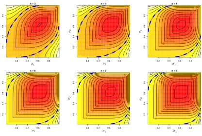
Figure 2: Contour curves of the values of||Mn||op ford= 2 and forn >2 as a function of λ1 andλ2,i.e., the two eigenvalues ofA. Ais assumed to be symmetric. Similar
results are obtained for higher-order cumulants.
also means that Mn is symmetric). Denote byλ1, . . . , λd to the eigenvalues ofA. That is,
σi = q
λ2
i and 0≤λ2i ≤1,i= 1, . . . , d. For a fixed cumulant of ordern we have that
||Mn||op = max
v∈S n Y j=1 h 1−λ2
vj
i 1−Qn
i=1λvi
+ (−1)n
n Y j=1
λvj
, (12)
whereS={1, . . . , d}n,|·|denotes absolute value, and we have employed standard properties
of the Kronecker product about eigenvalues and eigenvectors (Laub, 2004). Note that this expression does not depend on the eigenvectors of A, but only on its eigenvalues.
Figure 2 shows, for symmetric A, the value of ||Mn||op for n = 3, . . . ,8, and d = 2
when the two eigenvalues of A range in the interval (−1,1). We observe that ||Mn||op is always smaller than one. As described before, this will lead to a reduction in the `2-norm
of the cumulants in the anti-causal direction due to (11), and will in consequence produce a Gaussianization effect on the distribution of the residuals. For n ≤ 2 it can be readily shown that||M1||op =||M2||op = 1.
In general, the matrixAneed not be symmetric. In this case,||M1||op=||M2||op = 1 as
0.2 0.4 0.6 0.8
0.2
0.4
0.6
0.8
n = 3
0.4 0.5
0.6
0.7
0.8
0.9
1
1 1.1
1.1
1.2
1.2
1.3
1.3 1.4
1.4
1
1
0.2 0.4 0.6 0.8
0.2
0.4
0.6
0.8
n = 4
0.4
0.5
0.6
0.7
0.8
0.9
1
1 1.1
1.1
1.2
1.2
1.3
1.3 1.4
1.4
1
1
0.2 0.4 0.6 0.8
0.2
0.4
0.6
0.8
n = 5
0.2
0.3 0.4
0.5
0.6
0.7
0.8
0.9
1
1 1.1
1.1
1.2
1.2 1.3
1.3
1
1
0.2 0.4 0.6 0.8
0.2
0.4
0.6
0.8
n = 6
0.2 0.3
0.4
0.5
0.6
0.7
0.8
0.9
1
1 1.1
1.1 1.2
1.2
1.3
1.3
1
1
0.2 0.4 0.6 0.8
0.2
0.4
0.6
0.8
n = 7
0.1
0.2 0.3
0.4
0.5
0.6
0.7
0.8 0.9
1
1 1.1
1.1
1.2
1.2
1.3 1
1
0.2 0.4 0.6 0.8
0.2
0.4
0.6
0.8
n = 8
0.1 0.2
0.3
0.4
0.5
0.6
0.7
0.8
0.9
1
1 1.1
1.1
1.2
1.2
1.3 1
1
Figure 3: Contour curves of the values of||Mn||op ford= 2 and forn >2 as a function of σ1 and σ2,i.e., the two singular values ofA. Ais not assumed to be symmetric.
The singular vectors ofA are chosen at random. A dashed blue line highlights the boundary of the region where||Mn||op is strictly smaller than one.
Figure 3 displays the values of||Mn||op, ford= 2, as the two singular values ofA,σ1 and
σ2, vary in the interval (0,1). The left singular vectors and the right singular vectors of A
are chosen at random. In this figure a dashed blue line highlights the boundary of the region where ||Mn||op is strictly smaller than one. We observe that for most values of σ1 and σ2, ||Mn||op is smaller than one, leading to a Gaussianization effect in the distribution of the
residuals in the anti-causal direction. However, for some singular values,||Mn||op is strictly larger than one. Of course, this does not mean that there is not such a Gaussianization effect also in those cases. The definition given for||Mn||opassumes that all potential vectors v represent valid cumulants of a probability distribution, which need not be the case in practice. For example, it is well known that cumulants exhibit some form of symmetry (McCullagh, 1987). This can be seen in the second order cumulant, which is a covariance matrix. The consequence is that||Mn||op is simply an upper bound on the reduction of the
`2-norm of the cumulants in the anti-causal model. Thus, we also expect a Gaussianization
0.2 0.4
0.6
0.8 0.2
0.4 0.6
0.8 1.0
1.2 1.4 1.6
0.2 0.4
0.6
0.8 0.2
0.4 0.6
0.8 1.0
1.2 1.4 1.6
Figure 4: (left) Value of||M2||op, ford= 2, as a function ofσ1andσ2,i.e., the two singular
values of A. (right) Actual ratio between ||vect(κ2(i))||2 and ||vect(κ2(˜i))||2,
ford= 2, as a function of σ1 and σ2. A is not assumed to be symmetric. The
singular vectors ofAare chosen at random.
The fact that ||Mn||op is only an upper bound is illustrated in Figure 4. This figure
considers the particular case of the second cumulantκ2(·), which can be analyzed in detail.
On the left plot the value of||M2||opis displayed as a function ofσ1 andσ2, the two singular
values of A. We observe that ||M2||op takes values that are larger than one. In this case
it is possible to evaluate in closed form the `2-norm of vect(κ2(i)) and vect(κ2(˜i)), i.e.,
the vectors that contain the second order cumulant of the residuals in each direction. In particular, it is well known that the second order cumulant is equal to the covariance matrix (McCullagh, 1987). In the causal direction, the covariance matrix of the residuals is C=
I−AAT, as shown in the previous paragraphs. The covariance matrix of the residuals in the anti-causal direction, denoted by ˜C, can be computed similarly. Namely, ˜C=I−ATA. These two matrices, i.e., Cand ˜C, respectively give k2(i) andk2(˜i). Furthermore, they
have the same singular values. This means that ||vect(k2(i))||2/||vect(k2(˜i))||2 = 1, as
illustrated by the right plot in Figure 4. Thus, ||M2||op is simply an upper bound on the
actual reduction of the `2-norm of the second order cumulant of the residuals in the
anti-causal direction. The same behavior is expected for ||Mn||op, with n >2. In consequence, one should expect that the cumulants of the distribution of the residuals of a model fitted in the anti-causal direction are smaller in magnitude. This will lead to an increased level of Gaussianity measured in terms of a reduction of the magnitude of the high-order cumulants.
2.3 Analysis of the Multivariate Case Based on Information Theory
section, they need not be whitened, only centered. Here we closely follow Section 2.4 of the work by Hyv¨arinen and Smith (2013) and extend their results to the multivariate case.
Under the assumptions specified earlier, the model in the causal direction isyi=Axi+ i, with xi⊥i and A = Cov(Y,X)Cov(X,X)−1. Similarly, the model in the anti-causal
direction isxi = ˜Ayi+ ˜i with ˜A= Cov(X,Y)Cov(Y,Y)−1. By making use of the causal
model it is possible to show that ˜i = (I−AA˜ )xi−A˜i, where I is the identity matrix.
Thus, the following equations are satisfied:
xi yi
=P
xi i
=
I 0 A I
xi i
, (13)
and
yi
˜ i
= ˜P
xi i
=
A I
I−AA˜ −A˜
xi i
. (14)
Let H(xi,yi) be the entropy of the joint distribution of the two random variables as-sociated with samples xi and yi. Because (13) is a linear transformation, we can use
the entropy transformation formula (Hyv¨arinen and Smith, 2013) to get that H(xi,yi)
= H(xi,i) + log|detP|, where detP = detI = 1. Thus, we have that H(xi,yi) =
H(xi,i). Conversely, if we use (14) we have H(yi,i) = H(xi,i) + log|det ˜P|, where
det ˜P= detA·det(−A˜ −(I−AA˜ )A−1I) =−detI=−1, under the assumption that A is
invertible. The result is that H(xi,yi) =H(yi,i) =H(xi,i).
Denote the mutual information between the cause and the noise withI(xi,i). Similarly,
let I(yi,˜i) be the mutual information between the random variables corresponding to the
observationsyi and ˜i. Then,
I(xi,i)−I(yi,˜i) =H(xi) +H(i)−H(xi,i)−H(yi)−H(˜i) +H(yi,˜i)
=H(xi) +H(i)−H(yi)−H(˜i). (15)
Furthermore, from the actual causal model assumed we know thatI(xi,i) = 0. By contrast,
we have that I(yi,˜i) ≥ 0, since both yi and ˜i depend on xi and i. We also know that
H(xi) = H(yi) because we have made the hypothesis that both X and Y follow the same
distribution. The result is that:
H(i)≤H(˜i), (16)
with equality iff the residuals are Gaussian. We note that an alternative but equivalent way to obtain this last result is to consider a multivariate version of Lemma 1 by Kpotufe et al. (2014), under the assumption of the same distribution for the cause and the effect. In particular, even though Kpotufe et al. (2014) assume univariate random variables, their work can be easily generalized to multiple variables.
Although the random variables corresponding to i and ˜i have both zero mean, they
need not have the same covariance matrix. Denote with Cov(i) and Cov(˜i) to these
matrices and let ˆi and ˆ˜i be the whitened residuals (i.e., the residuals multiplied by the
Cholesky factor of the inverse of the corresponding covariance matrix). Then,
H(ˆi)≤H(ˆ˜i)−
1
2log|detCov(˜i)|+ 1
As shown in Appendix A, although not equal, the matrices Cov(i) and Cov(˜i) have the
same determinant. Thus, the two determinants cancel in the equation above. This gives,
H(ˆi)≤H(ˆ˜i). (18)
The consequence is that the entropy of the whitened residuals in the anti-causal direction is expected to be higher or equal than the entropy of the whitened residuals in the causal direction. Because the Gaussian distribution is the continuous distribution with the highest entropy for a fixed covariance matrix, we conclude that the level of Gaussianity of the residuals in the anti-causal direction, measured in terms of differential entropy, has to be larger or equal to the level of Gaussianity of the residuals in the causal direction.
In summary, if the causal relation between the two identically distributed random vari-ables X and Y is linear the residuals of a least squares fit in the anti-causal direction are more Gaussian than those of a linear fit in the causal direction. This Gaussianization can be characterized by a reduction of the magnitude of the corresponding high-order cumulants (although we have not formally proved this, we have provided some evidence that this is the case) and by an increase of the entropy (we have proved this in this section). A causal inference method can take advantage of this asymmetry to determine the causal direction. In particular, statistical tests based on measures of Gaussianity can be used for this pur-pose. However and importantly, these measures of Gaussianity need not be estimates of the differential entropy or the high-order cumulants. In particular, the entropy is a quantity that is particularly difficult to estimate in practice (Beirlant et al., 1997). The same occurs with the high-order cumulants. Their estimators involve high-order moments, and hence suffer from high variance.
When the distribution of the residuals in (6) is Gaussian, the causal direction cannot be identified. In this case, it is possible to show that the distribution of the reversed residuals ˜
i, the cause xi, and the effect yi, is Gaussian as a consequence of (9) and (11). This
non-identifiability agrees with the general result of Shimizu et al. (2006), which indicates that non-Gaussian distributions are strictly required in the disturbance variables to carry out causal inference in linear models with additive independent noise.
Finally, the fact that the Gaussianization effect is also expected in the multivariate case suggests a method to address causal inference problems in which the relationship between cause and effect is non-linear: It consists in mapping each observationxi andyi to a vector
in an expanded feature space. One can them assume that the non-linear relation in the original input space is linear in the expanded feature space and compute the residuals of kernel ridge regressions in both directions. The direction in which the residuals are less Gaussian is identified as the causal one.
3. A Feature Expansion to Address Non-linear Causal Inference Problems
We now proceed to relax the assumption that the causal relationship between the unidi-mensional random variables X and Y is linear. For this purpose, instead of working in the original space in which the samples{(xi, yi)}Ni=1 are observed, we will assume that the
model is linear in some expanded feature space {(φ(xi), φ(yi))}Ni=1 for some mapping
func-tion φ(·) : R → Rd. Importantly, this map preserves the property that if x
equally distributed, so will be φ(xi) and φ(yi). According to the analysis presented in the
previous section, the residuals of a linear model in the expanded space should be more Gaus-sian in the anti-causal direction than the residuals of a linear model in the causal direction, based on an increment of the differential entropy and on a reduction of the magnitude of the cumulants. The assumption we make is that the non-linear relation between X and Y
in the original input space is linear in the expanded feature space.
In this section we focus on obtaining the normalized residuals of linear models formu-lated in the expanded feature space. For this purpose, we assume that a kernel function k(·,·) can be used to evaluate dot products in the expanded feature space. In particular, k(xi, xj) = φ(xi)Tφ(xj) andk(yi, yj) =φ(yi)Tφ(yj) for arbitrary xi and xj and yi and yj.
Furthermore, we will not assume in general thatφ(xi) andφ(yi) have been whitened, only
centered. Whitening is a linear transformation which is not expected to affect to the level of Gaussianity of the residuals. However, once these residuals have been obtained they will be whitened in the expanded feature space. Later on we describe how to center the data in the expanded feature space. For now on, we will assume this step has already been done.
3.1 Non-linear Model Description and Fitting Process
Assume that the relation between X and Y is linear in an expanded feature space
φ(yi) =Aφ(xi) +i, i ⊥xi, (19)
wherei is i.i.d. non-Gaussian additive noise.
GivenN paired observations{(xi, yi)}Ni=1 drawn i.i.d. fromP(X,Y), define the matrices Φx = (φ(x1), . . . , φ(xN)) and Φy = (φ(y1), . . . , φ(yN)) of size d×N. The estimate of A
that minimizes the sum of squared errors is ˆA=ΓΣ−1, whereΓ=ΦyΦTx andΣ=ΦxΦTx. Unfortunately, when d > N, where dis the number of variables in the feature expansion, the matrix Σ−1 does not exist and ˆA is not unique. This means that there is an infinite number of solutions for ˆAwith zero squared error.
To avoid the indetermination described above and also to alleviate over-fitting, we pro-pose a regularized estimator. Namely,
L(A) =
N X
i=1
1
2||φ(yi)−Aφ(xi)||
2 2+τ
1 2||A||
2
F, (20)
where || · ||2 denotes the `2-norm and || · ||F denotes the Frobenius norm. In this last
expression τ >0 is a parameter that controls the amount of regularization. The minimizer of (20) is ˆA=ΓΣ−1, whereΓ=ΦyΦxTandΣ=τI+ΦxΦTx. The larger the value ofτ, the closer the entries of ˆAare to zero. Furthermore, using the matrix inversion lemma we have thatΣ−1=τ−1I−τ−1ΦxV−1ΦxT, whereV= (τI+Kx,x)−1 and Kx,x=ΦTxΦx is a kernel matrix whose entries are given by k(xi, xj). After some algebra it is possible to show that
ˆ
A=ΓΣ−1 =ΦyVΦTx, (21)
3.2 Obtaining the Matrix of Inner Products of the Residuals
A first step towards obtaining the whitened residuals in feature space (which will be required for the estimation of their level of Gaussianity) is to compute the matrix of inner products of these residuals (kernel matrix). For this, we define i=φ(yi)−Aˆφ(xi). Thus,
Ti j = h
φ(yi)−Aˆφ(xi)
iTh
φ(yj)−Aˆφ(xj) i
=φ(yi)Tφ(yj)−φ(yi)TAˆφ(xj)−φ(xi)TAˆφ(yj) +φ(xi)TAˆAˆφ(xj), (22)
for two arbitrary residuals i and j in feature space. In general, if we denote with K to
the matrix whose entries are given by Ti j and defineKy,y =ΦTyΦy, we have that
K=Ky,y−Ky,yVKx,x−Kx,xVKy,y+Kx,xVKy,yVKx,x, (23)
where we have used the definition of ˆAin (21). This expression only depends on the kernel matrices Kx,x and Ky,y and the matrixV, and can be computed with costO(N3).
3.3 Centering the Input Data and Centering and Whitening the Residuals
An assumption made in Section 2 was that the samples of the random variables X and
Y are centered, i.e., they have zero mean. In this section we show how to carry out this centering process in feature space. Furthermore, we also show how to center the residuals of the fitting process, which are also whitened. Whitening is a standard procedure in which the data are transformed to have the identity matrix as the covariance matrix. It also corresponds to projecting the data onto all the principal components, and scaling them to have unit standard deviation.
We show how to center the data in feature space. For this, we follow Sch¨olkopf et al. (1997) and work with:
˜
φ(xi) =φ(xi)−
1 N
N X j=1
φ(xj), φ˜(yi) =φ(yi)−
1 N
N X j=1
φ(yj). (24)
The consequence is that now the kernel matricesKx,x and Ky,y are replaced by
˜
Kx,x=Kx,x−1NKx,x−Kx,x1N +1NKx,x1N,
˜
Ky,y=Ky,y−1NKy,y−Ky,y1N+1NKy,y1N, (25)
where 1N is aN ×N matrix with all entries equal to 1/N. The residuals can be centered
also in a similar way. Namely, ˜K =K−1NK−K1N +1NK1N.
We now explain the whitening of the residuals, which are now assumed to be centered. This process involves the computation of the eigenvalues and eigenvectors of the d×d co-variance matrixCof the residuals. This is done as in kernel PCA (Sch¨olkopf et al., 1997). Denote by ˜i to the centered residuals. The covariance matrix is C = N−1PNi=1˜i˜Ti.
The eigenvector expansion implies that Cvi =λivi, where vi denotes the i-th eigenvector
and λi the i-th eigenvalue. The consequence is that N−1PNk=1˜k˜Tkvi = λivi. Thus, the
eigenvectors can be expressed as a combination of the residuals. Namely, vi=PN
where bi,j = N−1˜Tjvi. Substituting this result in the previous equation we have that
N−1PN
k=1˜k˜kTPNj=1bi,j˜j =λiPNj=1bi,j˜j. When we multiply both sides by ˜Tl we obtain
N−1PN
k=1˜Tl ˜k˜Tk
PN
j=1bi,j˜j =λi
PN
j=1bi,j˜Tl ˜j, forl= 1, . . . d, which is written in terms
of kernels as ˜KKbi˜ =λiNKbi˜ , where bi = (bi,1, . . . , bi,N)T. A solution to this problem
is found by solving the eigenvalue problem ˜Kbi =λiNbi. We also require that the
eigen-vectors have unit norm. Thus, 1 =vTi vi =PNj=1
PN
k=1bi,jbi,k˜Tj˜k=biTK˜bi=λiNbTi bi,
which means that bi has norm 1/ √
λiN. Consider now that ˜bi is one eigenvector of ˜K.
Then, bi = 1/ √
λiNb˜i. Similarly, let ˜λi be an eigenvalue of ˜K. Then λi = ˜λi/N. In
summary,λi andbi,j, withi= 1, . . . , N and j= 1, . . . , N can be found with costO(N3) by
finding the eigendecomposition of ˜K.
The whitening process is carried out by projecting each residual ˜konto each eigenvector vi and then multiplying by 1/
√
λi. The correspondingi-th component for thek-th residual,
denoted by Zk,i, is Zk,i = 1/ √
λivTi ˜k = 1/ √
λiPNj=1bi,j˜Tj˜k, and in consequence, the
whitened residuals areZ= ˜KBD=NBD−1 = √
NB˜, whereBis a matrix whose columns contain each bi, ˜B is a matrix whose columns contain each ˜bi and D is a diagonal matrix
whose entries are equal to 1/√λi. Each row ofZnow contains the whitened residuals.
3.4 Inferring the Most Likely Causal Direction
After having trained the model and obtained the matrix of whitened residuals Z in each direction, a suitable Gaussianity test can be used to determine the correct causal relation between the variables X and Y. Given the theoretical results of Section 2 one may be tempted to use tests based on entropy or cumulants estimation. Such tests may perform poorly in practice due to the difficulty of estimating high-order cumulants or differential entropy. In particular, the estimators of the cumulants involve high-order moments and hence, suffer from high variance. As a consequence, in our experiments we use a statistical test for Gaussianity based on theenergy distance (Sz´ekely and Rizzo, 2005), which has good power, is robust to noise, and does not have any adjustable hyper-parameters. Furthermore, in Appendix B we motivate that in the anti-causal direction one should also expect a smaller energy distance to the Gaussian distribution.
Assume X and Y are two independent random variables whose probability distribution functions are F(·) andG(·). The energy distance between these distributions is defined as
D2(F, G) = 2E[||X − Y||]−E[||X − X0||]−E[||Y − Y0||], (26) where || · || denotes some norm, typically the `2-norm; X and X0 are independent and
identically distributed (i.i.d.); Y and Y0 are i.i.d; and E denotes expected value. The
energy distance satisfies all axioms of a metric and hence characterizes the equality of distributions. Namely, D2(F, G) = 0 if and only if F = G. Furthermore, in the case of univariate random variables the energy distance is twice the Cram´er-von Mises distance given byR
(F(x)−G(x))2dx.
Assume X= (x1, . . . ,xN)T is a matrix that contains N random samples (one per each
that is described by Sz´ekely and Rizzo (2005) is:
Energy(X) =N
2 N
N X j=1
E[||xj− Y||]−E[||Y − Y0||]− 1
N2 N X j,k=1
||xj−xk||
, (27)
where Y and Y0 are independent random variables distributed as N(·|0,I) and E denotes
expected value. Furthermore, the required expectations with respect to the Gaussian ran-dom variables Y and Y0 can be efficiently computed as described by Sz´ekely and Rizzo (2005). The idea is that if f is similar to a Gaussian density N(·|0,I), then Energy(X) is close to zero. Conversely, the null hypothesisH0 is rejected for large values of Energy(X).
The data to test for Gaussianity is in our case Z,i.e., the matrix of whitened residuals, which has size N ×N. Thus, the whitened residuals have N dimensions. The direct introduction of these residuals into a statistical test for Gaussianity is not expected to provide meaningful results, as a consequence of the high dimensionality. Furthermore, in our experiments we have observed that it is often the case that a large part of the total variance is explained by the first principal component (see the supplementary material for evidence supporting this). That is, λi, i.e., the eigenvalue associated to the i-th principal
component, is almost negligible for i ≥ 2. Additionally, we motivate in Appendix C that one should also obtain more Gaussian residuals, after projecting the data onto the first principal component, in terms of a reduction of the magnitude of the high-order cumulants. Thus, in practice, we consider only the first principal component of the estimated residuals in feature space. This is the component i with the largest associated eigenvalue λi. We
denote such N-dimensional vector byz.
Let zx→y be the vector of coefficients of the first principal component of the residuals
in feature space when the linear fit is performed in the directionX → Y. Let zy→x be the vector of coefficients of the first principal component of the residuals in feature space when the linear fit is carried out in the directionY → X. We define the measure of Gaussianization of the residuals asG= Energy(zx→y)/N−Energy(zy→x)/N, where Energy(·) computes the statistic of the energy distance test for Gaussianity described above. Note that we divide each statistic by N to cancel the corresponding factor that is considered in (27). Since in this test larger values for the statistic corresponds to larger deviations from Gaussianity, if
G >0 the direction X → Y is expected to be more likely the causal direction. Otherwise, the directionY → X is preferred.
The variance of G will depend on the sample size N. Thus, ideally one should use the difference between thep-values associated to each statistic as the confidence in the decision taken. Unfortunately, computing these p-values is expensive since the distribution of the statistic under the null hypothesis must be approximated via random sampling. In our experiments we measure the confidence of the decision in terms of the absolute value of G, which is faster to obtain and we have found to perform well in practice.
3.5 Parameter Tuning and Error Evaluation
Assume that a squared exponential kernel is employed in the method described above. This means that k(xi, xj) = exp −γ(xi−xj)2
in the method described. These are the ridge regression regularization parameter τ and the kernel bandwidth γ. They must be tuned in some way to produce the best possible fit in each direction. The method chosen to guarantee this is a grid search guided by a 10-fold cross-validation procedure, which requires computing the squared prediction error over unseen data. In this section we detail how to evaluate these errors.
Assume that M new paired data instances are available for validation. Let the two matrices Φynew = (φ(ynew
1 ), . . . , φ(yMnew)) and Φxnew = (φ(xnew
1 ), . . . , φ(xnewM )) summarize
these data. Define newi =φ(yinew)−Aˆφ(xnewi ). After some algebra, it is possible to show that the sum of squared errors for the new instances is:
E=
M X
i=1
(newi )Tnewi = trace
Kynew,ynew−Kynew,yVKTxnew,x−
Kxnew,xVKTynew,y+Kxnew,xVKy,yVKTxnew,x
. (28)
where Kynew,ynew =ΦTynewΦynew,Kynew,y =ΦTynewΦy and Kx,xnew =ΦTxΦxnew.
Of course, the new data must be centered before computing the error estimate. This process is similar to the one described in the previous section. In particular, centering can be simply carried out by working with the modified kernel matrices:
˜
Kxnew,x=Kxnew,x−MNKx,x−Kxnew,x1N+MNKx,x1N,
˜
Kynew,y =Kynew,y−MNKy,y−Kynew,y1N +MNKy,y1N,
˜
Kynew,ynew =Kynew,ynew−MNKy,ynew−Kynew,yMTN +MNKy,yMTN, (29)
where MN is a matrix of sizeM ×N with all components equal to 1/N. In this process, the averages employed for the centering step are computed using only the observed data.
A disadvantage of the squared error is that it strongly depends on the kernel bandwidth parameter γ. This makes it difficult to choose this hyper-parameter in terms of such a performance measure. A better approach is to choose bothγandτ in terms of the explained variance by the model. This is obtained as follows: Explained-Variance = 1−E/MVarynew,
whereE denotes the squared prediction error and Varynew the variance of the targets. The
computation of the errorEis done as described previously and Varynewis simply the average
of the diagonal entries in ˜Kynew,ynew.
3.6 Finding Pre-images for Illustrative Purposes
The kernel method described above expresses its solution as feature maps of the original data points. Since the feature map φ(·) is usually non-linear, we cannot guarantee the existence of a pre-image under φ(·). That is, a point y such that φ(y) = ˆAφ(x), for some input pointx. An alternative to amend this issue is to find approximate pre-images, which can be useful to make predictions or plotting results (Sch¨olkopf and Smola, 2002). In this section we describe how to find this approximate pre-images.
Assume that we have a new data instance xnew for which we would like to know the
feature space is:
φ(ynew) =ΦyVΦTxφ(xnew) =ΦyVkx,xnew =
n X
i=1
αiφ(yi), (30)
where kx,xnew contains the kernel evaluations between each entry in x (i.e., the observed
samples of the random variable X) and the new instance. Finally, each αi is given by a
component of the vector Vkx,xnew. The approximate pre-image of φ(ynew), ynew, is found
by solving the following optimization problem:
ynew= arg min u
||φ(ynew)−φ(u)||22 = arg min u
−2αTky,u+k(u, u), (31)
whereky,uis a vector with the kernel values between eachyiandu, andk(u, u) =φ(u)Tφ(u).
This is a non-linear optimization problem than can be solved approximately using standard techniques such as gradient descent. In particular, the computation of the gradient of ky,u
with respect tou is very simple in the case of the squared exponential kernel.
4. Data Transformation and Detailed Causal Inference Algorithm
The method for causal inference described in the previous section relies on the fact that both random variables X and Y are equally distributed. In particular, if this is the case, φ(xi) and φ(yi), i.e., the maps of xi and yi in the expanded feature space, will also be
equally distributed. This means that under such circumstances one should expect residuals that are more Gaussian in the anti-causal direction due to a reduction of the magnitude of the high order cumulants and an increment of the differential entropy. The requirement that
X and Y are equally distributed can be easily fulfilled in the case of continuous univariate data by transformingx, the samples ofX, to have the same empirical distribution asy, the samples of Y.
Consider x = (x1, . . . , xN)T and y = (y1, . . . , yN)T to be N paired samples of X and Y, respectively. To guarantee the same distribution for these samples we only have to replace xby ˜x, where each component of ˜x, ˜xi, is given by ˜xi = ˆFy−1( ˆFx(xi)), with ˆFy−1(·)
the empirical quantile distribution function of the random variable Y, estimated using y. Similarly, ˆFx(·) is the empirical cumulative distribution function of X, estimated using x.
This operation is known as the probability integral transform.
One may wonder why should x be transformed instead of y. The reason is that by transformingxthe additive noise hypothesis made in (1) and (6) is preserved. In particular, we have that yi=f( ˆFx−1( ˆFy(˜xi))) +i. On the other hand, if yis transformed instead, the
additive noise model will generally not be valid anymore. More precisely, the transformation that computes ˜y in such a way that it is distributed asx is ˜yi = ˆFx−1( ˆFy(yi)), ∀i. Thus,
under this transformation we have that ˜yi = ˆFx−1( ˆFy(f(xi) +i)), which will lead to the
violation of the additive noise model.
of x, the Gaussianization effect of the residuals is not as high as when x is transformed, as a consequence of the violation of the additive noise model. This will allow to determine the causal direction. We do not have a theoretical result confirming this statement, but the good results obtained in Section 6.1 indicate that this is the case.
The details of the complete causal inference algorithm proposed are given in Algorithm 1. Besides a causal direction,e.g.,X → Y orY → X, this algorithm also outputs a confidence level in the decision made which is defined as max(|Gx˜|,|Gy˜|), whereG˜x= Energy(zx→y˜ )/N−
Energy(zy→x˜)/N denotes the estimated level of Gaussianization of the residuals when x
is transformed to have the same distribution as y. Similarly, Gy˜ = Energy(zy→x˜ )/N −
Energy(zy→x˜ )/N denotes the estimated level of Gaussianization of the residuals when x
and y are swapped and y is transformed to have the same distribution as x. Here z˜x→y
contains the first principal component of the residuals in the expanded feature space when trying to predict y using ˜x. The same applies for zy→x˜, zy→x˜ and zx→y˜. However, the
residuals are obtained this time when trying to predict ˜x using y, when trying to predict
x using ˜y and when trying to predict ˜y using x, respectively. Recall that the reason for keeping only the first principal component of the residuals is described in Section 3.4.
Assume |Gx˜| > |Gy˜|. In this case we prefer the transformation of x to guarantee that
the cause and the effect have the same distribution. The reason is that it leads to a higher level of Gaussianization of the residuals, as estimated by the energy statistical test. Now consider that Gx˜ > 0. We prefer the direction X → Y because the residuals of a fit in
that direction are less Gaussian and hence have a higher value of the statistic of the energy test. By contrast, if Gx˜ < 0 we prefer the direction Y → X for the same reason. In the
case that |Gx˜| < |Gy˜| the reasoning is the same and we prefer the transformation of y.
However, because we have swapped xand yfor computing Gy˜, the decision is the opposite as the previous one. Namely, if Gy˜ > 0 we prefer the direction Y → X and otherwise we prefer the direction X → Y. The confidence in the decision (i.e., the estimated level of Gaussianization) is always measured by max(|Gx˜|,|Gy˜|).
The algorithm uses a squared exponential kernel with bandwidth parameter γ and the actual matrices ˆAx→y˜ and ˆAy→x˜, of potentially infinite dimensions, need not be evaluated in
closed form in practice. As indicated in Section 3, all computations are carried out efficiently with cost O(N3) using inner products, which are evaluated in terms of the corresponding
kernel function. All hyper-parameters, i.e.,τ andγ, are chosen using a grid search method guided by a 10-fold cross-validation process. This search maximizes the explained variance of the left-out data and 10 potential values are considered for bothτ and γ.
5. Related Work
Algorithm 1:Causal Inference Based on the Gaussianity of the Residuals (GR-AN) Data: Paired samplesxandy from the random variablesX and Y.
Result: An estimated causal direction alongside with a confidence level.
1 Standardizexandy to have zero mean and unit variance;
2 Transformxto compute ˜x; // This guarantees that x˜ is distributed as y. 3 Aˆx˜→y←FitModel(˜x,y) ; // This also finds the hyper-parameters τ and γ.
4 z˜x→y ←ObtainResiduals(˜x,y,Aˆ˜x→y) ; // First PCA component in feature space.
5 Aˆy→x˜←FitModel(y,x) ;˜ // Fit the model in the other direction 6 zy→x˜←ObtainResiduals(y,x˜,Aˆy→x˜) ; // First PCA component in feature space. 7 G˜x←Energy(zx˜→y)/N−Energy(zy→x˜)/N ; // Get the Gaussianization level. 8 Swapx andyand repeat lines 2-7 of the algorithm to computeGy˜.
9 if |G˜x|>|G˜y|then
10 if G˜x>0 then
11 Output: X → Y with confidence |G˜x|
12 else
13 Output: Y → X with confidence |G˜x|
14 end
15 else
16 if G˜y>0then
17 Output: Y → X with confidence |G˜y|
18 else
19 Output: X → Y with confidence |G˜y|
20 end
21 end
some advantages of using statistical tests based on measures of Gaussianity to determine the temporal direction of a time series, as a practical alternative to statistical tests based on the independence of the cause and the residual. The motivation for these advantages is that the former tests are one-sample tests while the later ones are two-sample tests.
The previous paper is extended by Morales-Mombiela et al. (2013) to consider mul-tidimensional AR processes. However, this work lacks a theoretical result that guaran-tees that the residuals obtained when fitting a vectorial AR process in the reversed (anti-chronological) direction will follow a distribution closer to a Gaussian distribution. In spite of this issue, extensive experiments with simulated data suggest the validity of such conjec-ture. Furthermore, a series of experiments show the superior results of the proposed rule to determine the direction of time, which is based on measures of Gaussianity, and compared with other state-of-the-art methods based on tests of independence.
order of. LINGAM assumes that x=Bx+e, where B is a matrix that can be permuted to strict lower triangularity if one knows the actual causal ordering in x, and eis a vector of non-Gaussian independent disturbance variables. Solving forx, one gets x=Ae, where
A= (I−B)−1. TheAmatrix can be inferred using ICA. Furthermore, given an estimate of
A, B can be obtained to find the corresponding connection strengths among the observed variables, which can then be used to determine the true causal ordering. LINGAM has been extended to consider linear relations among groups of variables (Entner and Hoyer, 2012; Kawahara et al., 2012).
In real-world data, causal relationships tend to be non-linear, a fact that questions the usefulness of linear methods. Hoyer et al. (2009) show that a basic linear framework for causal inference can be generalized to non-linear models. For non-linear models with additive noise, almost any non-linearities (invertible or not) will typically yield identifiable models. In particular, Hoyer et al. (2009) assume thatyi =f(xi)+i, wheref(·) is a possibly
non-linear function, xi is the cause variable, andi is some independent and random noise.
The proposed causal inference mechanism consists in performing a non-linear regression on the data to get an estimate of f(·), ˆf(·), and then calculate the corresponding residuals ˆ
i=yi−fˆ(xi). Then, one may test whether ˆi is independent ofxior not. The same process
is repeated in the other direction. The direction with the highest level of independence is chosen as the causal one. In practice, the estimate ˆf(·) is obtained using Gaussian processes for regression, and the HSIC test (Gretton et al., 2008) is used as the independence criterion. This method has obtained good performance results (Janzing et al., 2012) and it has been extended to address problems where the model is yi = h(f(xi) +i), for some invertible
function h(·) (Zhang and Hyv¨arinen, 2009). A practical difficulty is however that such a model is significantly harder to fit to the data.
In the work by Mooij et al. (2010), a method for causal inference is proposed based on a latent variable model, used to incorporate the effects of un-observed noise. In this context, it is considered that the effect variable is a function of the cause variable and an independent noise term, not necessarily additive, that is, yi = f(xi, i), where xi is the
cause variable and i is some independent and random noise. The causal direction is then
inferred using standard Bayesian model selection. In particular, the preferred direction is the one under which the corresponding model has the largest marginal likelihood, where the marginal likelihood is understood as a proxy for the Kolmogorov complexity. This method suffers from several implementation difficulties, including the intractability of the marginal likelihood computation. However, it has shown encouraging results on synthetic and real-world data.
Janzing et al. (2010) consider the problem of inferring linear causal relations among multi-dimensional variables. The key point here is to use an asymmetry between the distri-butions of the cause and the effect that occurs if the covariance matrix of the cause and the matrix mapping the cause to the effect are independently chosen. This method exhibits the nice property that applies to both deterministic and stochastic causal relations, provided that the dimensionality of the involved random variables is sufficiently high. The method assumes thatyi =Axi+i, wherexi is the cause andi is additive noise. Namely, denote
yi are swapped. The asymmetry described states that ∆x→y should be close to zero while
∆y→x should not. Thus, if|∆x→y|>|∆y→x|, xi is expected to be the cause. Otherwise, the variables in yi are predicted to be cause instead. Finally, a kernelized version of this
method is also described by Chen et al. (2013).
Most of the methods introduced in this section assume some form of noise in the gen-erative process of the effect. Thus, their use is not justified in the case of noiseless data. Janzing et al. (2012) describe a method to deal with these situations. In particular, the method makes use of information geometry to identify an asymmetry that can be used for causal inference. The asymmetry relies on the idea that the marginal distribution of the cause variable, denoted byp(x), is expected to be chosen independently from the mapping mechanism producing the effect variable, denoted by the conditional distribution p(y|x). Independence is defined here as orthogonality in the information space, which allows to describe a dependence that occurs between p(y) and p(x|y) in the anti-causal direction. This dependence can be then used to determine the causal order. A nice property of this method is that this asymmetry between the cause and the effect becomes very simple if both random variables are deterministically related. Remarkably, the method also performs very well in noisy scenarios, although no theoretical guarantees are provided in this case.
A similar method for causal inference to the last one is described by Chen et al. (2014). These authors also consider thatp(x) andp(y|x) fulfill some sort of independence condition, and that this independence condition does not hold for the anti-causal direction. Based on this, they define an uncorrelatedness criterion between p(x) and p(y|x), and show an asymmetry between the cause and the effect in terms of a certain complexity metric on p(x) and p(y|x), which is less than the same complexity metric on p(y) and p(x|y). The complexity metric is calculated in terms of a reproducing kernel Hilbert space embedding (EMD) of probability distributions. Based on the complexity metric, the authors propose an efficient kernel-based algorithm for causal discovery.
In Section 2.3 we have shown that in the multivariate case one should expect higher entropies in the anti-causal direction. Similar results have been obtained in the case of non-linear relations and the univariate data case (Hyv¨arinen and Smith, 2013; Kpotufe et al., 2014). Assumex, y∈Rand the actual causal model to bey=f(x) +d, withx⊥dandf(·) an arbitrary function. Letebe the residual of a fit performed in the anti-causal direction. Section 5.2 of the work by Hyv¨arinen and Smith (2013) shows that the likelihood ratioR of each model (i.e., the model fitted in the causal direction and the model fitted in the anti-causal direction) converges in the presence of infinite data to the difference between the sum of the entropies of the independent variable and the residual in each direction. Namely, R → −H(x) −H(d/σd) +H(y) +H(e/σe) + logσd−logσe, where σd and σe
denote the standard deviation of the errors in each direction. IfR >0, the causal direction is chosen. By contrast, if R < 0 the anti-causal direction is preferred. The process of evaluating R involves the estimation of the entropies of four univariate random variables,
even in one dimension (Beirlant et al., 1997). Thus, the NLME method is adapted in an
ad-hoc manner with the aim of obtaining better results in certain difficult situations with sparse residuals. More precisely, if H(x) and H(y) are ignored and Laplacian residuals are assumedR→logσe−logσd. That is, the model with the minimum error is preferred. The
errors are estimated however in terms of the absolute deviations (because of the Laplacian assumption). This method is called mean absolute deviation (MAD). Finally, Kpotufe et al. (2014) show the consistency of the noise additive model, give a formal proof forR ≥0 (see Lemma 1), and propose to estimate H(x),H(y), H(d) andH(e) using kernel density estimators. Note that if x and y are equally distributed, H(x) = H(y) and the condition R ≥ 0 implies H(e) ≥ H(d). Nevertheless, σd and σe are in general different (see the
supplementary material for an illustrative example). This means that in the approach of Hyv¨arinen and Smith (2013) and Kpotufe et al. (2014) it is not possible to make a decision directly on the basis of a Gaussianization effect on the residuals.
The proposed method GR-AN, introduced in Section 4, differs from the approaches de-scribed in the previous paragraph in that it does not have to deal with the estimation of four univariate entropies, which can be a particularly difficult task. By contrast, it relies on statistical tests of deviation from Gaussianity to infer the causal direction. Further-more, the tests employed in our method need not be directly related to entropy estimation. This is particularly the case of the energy test suggested in Section 3.4. Not having to estimate differential entropies is an advantage of our method confirmed by the results that are obtained in the experiments section. In particular, we have empirically observed that that GR-AN performs better than the two methods for causal inference NLME and MAD that have been described in the previous paragraph. GR-AN also performs better than GR-ENT, a method that uses, instead of statistical tests of Gaussianity, a non-parametric estimator of the entropy (Singh et al., 2003).
6. Experiments
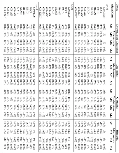
the empirical estimate of the fourth cumulant (kurtosis) to determine the causal direction (it chooses the direction with the largest estimated fourth cumulant); and GR-ENT, which uses a non-parametric estimator of the entropy (Singh et al., 2003) to determine the causal direction (the direction with the smallest entropy is preferred);
The hyper-parameters of the different methods are set as follows. In LINGAM, we use the parameters recommended by the implementation provided by the authors. In IR-AN, NLME and MAD we employ a Gaussian process whose hyper-parameters are found by type-II maximum likelihood. Furthermore, in IR-AN the HSIC test is used to assess independence between the causes and the residuals. In NLME the entropy estimator is the one described by Hyv¨arinen (1998). In IGCI, we test different normalizations (uniform and Gaussian) and different criteria (entropy or integral) and report the best observed result. In EMD and synthetic data, we follow Chen et al. (2014) to select the hyper-parameters. In EMD and real-world data, we evaluate different hyper-parameters and report the results for the best combination found. In GR-AN, GR-K4 and GR-ENT the hyper-parameters are found via cross-validation, as described in Section 4. The number of neighbors in the entropy estimator of GR-ENT is set to 10, a value that we have observed to give a good trade-off between bias and variance. Finally, in GR-AN, GR-K4, and GR-ENT we transform the data so that both variables are equally distributed, as indicated in Section 4.
The confidence in the decision is computed as indicated by Janzing et al. (2012). More precisely, in LINGAM the confidence is given by the maximum absolute value of the entries in the connection strength matrixB. In IGCI we employ the absolute value of the difference between the corresponding estimates (entropy or integral) in each direction. In IR-AN the confidence level is obtained as the maximum of the twop-values of the HSIC test. In EMD we use the absolute value of the difference between the estimates of the corresponding complexity metric in each direction, as described in (Chen et al., 2014). In NLME and MAD the confidence level is given by the absolute value of the difference between the outputs of the entropy estimators in each direction (Hyv¨arinen and Smith, 2013). In GR-K4 we use the absolute difference between the estimated fourth cumulants. In GR-ENT we use the absolute difference between the estimates of the entropy. Finally, in GR-AN we follow the details given in Section 4 to estimate the confidence in the decision.
To guarantee the exact reproducibility of the different experiments described in this paper, the source-code for all methods and data sets is available in the public repository
https://bitbucket.org/dhernand/gr_causal_inference.
6.1 Experiments with Synthetic Data
We carry out a first batch of experiments on synthetic data. In these experiments, we employ the four causal mechanisms that mapX toY described by Chen et al. (2014). They involve linear and non-linear functions, and additive and multiplicative noise effects: