Dimension Reduction in Text Classification with Support Vector Machines

Dimension Reduction in Text Classification

with Support Vector Machines

Hyunsoo Kim [email protected]

Peg Howland [email protected]

Haesun Park [email protected]

Department of Computer Science and Engineering University of Minnesota

200 Union Street S.E., 4-192 EE/CS Building Minneapolis MN 55455, USA

Editor: Nello Christianini

Abstract

Support vector machines (SVMs) have been recognized as one of the most successful classifica-tion methods for many applicaclassifica-tions including text classificaclassifica-tion. Even though the learning ability and computational complexity of training in support vector machines may be independent of the dimension of the feature space, reducing computational complexity is an essential issue to effi-ciently handle a large number of terms in practical applications of text classification. In this paper, we adopt novel dimension reduction methods to reduce the dimension of the document vectors dramatically. We also introduce decision functions for the centroid-based classification algorithm and support vector classifiers to handle the classification problem where a document may belong to multiple classes. Our substantial experimental results show that with several dimension reduction methods that are designed particularly for clustered data, higher efficiency for both training and testing can be achieved without sacrificing prediction accuracy of text classification even when the dimension of the input space is significantly reduced.

Keywords: dimension reduction, support vector machines, text classification, linear discriminant analysis, centroids

1. Introduction

Text classification is a supervised learning task for assigning text documents to pre-defined classes of documents. It is used to find valuable information from a huge collection of text documents available in digital libraries, knowledge databases, the world wide web (WWW), and company-wide intranets, to name a few. Several characteristics have been observed in vector space based methods for text classification (20; 21), including the high dimensionality of the input space, sparsity of document vectors, linear separability in most text classification problems, and the belief that few features are irrelevant. It has been conjectured that an aggressive dimension reduction may result in a significant loss of information, and therefore, result in poor classification results (13).

C is

max αi

n

∑

αi−

1 2

n

∑

αiαjyiyjK(xi,xj), (1)

s.t. n

∑

αiyi=0, 0≤αi≤C, i=1, . . . ,n.

The kernel function

K(xi,xj) =<φ(xi),φ(xj)>,

where <, > denotes an inner product between two vectors, is introduced to handle nonlinearly separable cases without any explicit knowledge of the feature mappingφ. The formulation (1) shows that the computational complexity of SVM training depends on the number of training data samples which is denoted as n. The dimension of the feature space does not influence the computational complexity of training or testing due to the use of the kernel function.

However, an often neglected fact is that the computational complexity of training depends on the dimension of the input space. This is clear when we consider some typical kernel functions such as the linear kernel

K(x,xi) =<x,xi>,

the polynomial kernel

K(x,xi) = [<x,xi>+β]d,

where d is the degree of the polynomial, and the Gaussian RBF (radial basis function) kernel

K(x,xi) =exp(₋γ_kx₋xi_k2),

whereγis a parameter to control. The evaluation of the kernel function depends on the dimension of

the input data, since the kernel functions contain the inner product of two input vectors for the linear

or polynomial kernels or the distance of two vectors for the Gaussian RBF kernel. Letα∗_i denote the optimal solution for (1). The optimal separating hyperplane f(x,α∗_{,b)also requires evaluation}

of the kernel function since

f(x,α∗,b) =

∑

xi∈SV

αiyiK(xi,x) +b

where SV denotes the set of support vectors, b is a bias given by

b=₋minyi=1<w∗,φ(xi)>+maxyi=−1<w∗,φ(xi)>

2

and

w∗= l

∑

yiαi∗φ(xi).

Therefore, more efficient testing as well as training is expected from dimension reduction.

Throughout the paper, we will assume that the document set is represented in an m_×n

In the next section, we review Latent Semantic Indexing (LSI) (2; 1), which uses the truncated singular value decomposition (SVD) as a low-rank approximation of A. Although the truncated SVD provides the closest approximation to A in Frobenius or L2 norm, LSI ignores the cluster structure while reducing the dimension of the data. In contrast, in Section 3, we review several dimension reduction methods that are especially effective for classification of clustered data: two methods based on centroids (16; 12), and one method which is a generalization of linear discriminant analysis (LDA) using the generalized singular value decomposition (GSVD) (10). With dimension reduction, computational complexity can be dramatically reduced for all classifiers including support vector machines and k-nearest neighbor classification. For k-nearest neighbor classification (kNN), the distances of vector pairs need to be computed when finding k nearest neighbors. Therefore, one can significantly reduce computational complexity by dimension reduction.

In many document data sets, documents can be assigned to more than one cluster upon clas-sification. To handle this problem more effectively, we introduce a threshold based extension of several classification algorithms in Section 4. Our numerical experiments illustrate that the cluster-preserving dimension reduction algorithms we employ reduce the data dimension without any sig-nificant loss of information. In fact, in many cases, they seem to have the effect of noise reduction, since prediction accuracy becomes better after dimension reduction when compared to that in the original high dimensional input space.

2. Low-Rank Approximation Using Latent Semantic Indexing

LSI is based on the assumption that there is some underlying latent semantic structure in the term-document matrix that is corrupted by the wide variety of words used in term-documents and queries. This is referred to as the problem of polysemy and synonymy (6). The basic idea is that if two document vectors represent the same topic, they will share many associating words with a keyword, and they will have very close semantic structures after dimension reduction via SVD. Thus LSI/SVD breaks the original relationship of the data into linearly independent components (6), where the original term vectors are represented by left singular vectors and document vectors by right singular vectors. That is, if l_≤rank(A), then

A_≈UlΣlVlT

, where the columns of Ul are the leading l left singular vectors,Σl is an l×l diagonal matrix with the l largest singular values in nonincreasing order along its diagonal, and the columns of Vl are the leading l right singular vectors. ThenΣlVlT is the reduced dimensional representation of A, or equivalently, a new document q_∈Rm×1can be represented in the l-dimensional space as ˆq=U_lTq.

Algorithm 1 : Centroid algorithm for Dimension Reduction

Given a data set A_∈Rm×n with p clusters and a vector q_∈Rm×1, this algorithm computes a p dimensional representation ˆq_∈Rp×1of q.

1. Compute the centroid ciof the ith cluster, 1≤i≤p

2. Set C=

c1 c2 ··· cp

3. Solve minˆqkC ˆq−qk2

Algorithm 2 : Orthogonal Centroid algorithm for Dimension Reduction

Given a data set A_∈Rm×n with p clusters and a vector q_∈Rm×1, this algorithm computes a p dimensional representation ˆq of q.

1. Compute the centroid ciof the ith cluster, 1≤i≤p

2. Set C=

c1 c2 _··· cp

3. Compute the reduced QR decomposition of C, which is C=QpR

4. ˆq=QT_pq

3. Dimension Reduction Algorithms for Clustered Data

To achieve greater efficiency in manipulating data represented in a high dimensional space, it is often necessary to reduce the dimension dramatically. In this section, several dimension reduction methods that preserve the cluster structure are reviewed. Each method attempts to choose a projec-tion to a reduced dimensional space that will capture the cluster structure of the data collecprojec-tion as much as possible.

3.1 Centroid-based Algorithms for Dimension Reduction of Clustered Data

Suppose we are given a data matrix A whose columns are grouped into p clusters. Instead of treating each column of the matrix A equally regardless of its membership in a specific cluster as in LSI/SVD, we want to find a lower dimensional representation Y of A so that the p clusters are preserved in Y . Given a term-document matrix, the problem is to find a transformation that maps each document vector in the m dimensional space to a vector in the l dimensional space for some

l<m. For this, either the dimension reducing transformation GT _∈Rl×m is computed explicitly or the problem is formulated as a rank reducing approximation where the given matrix A is to be decomposed into two matrices B and Y . That is,

A_≈BY (2)

the least squares problem (8; 12; 16)

min

B,Y kBY−AkF. (3) Any given document q_∈Rm×1 can be transformed to the lower dimensional space by solving the minimization problem

min

ˆq_∈Rl×1kB ˆq−qk2. (4)

Latent Semantic Indexing that utilizes the SVD (LSI/SVD) can be viewed as a variation of the model (2) with B=Ul (16), where UlΣlVlT is the rank l truncated SVD of A. Then ˆq=UlTq is obtained by solving the least squares problem

min

ˆq∈Rl×1kB ˆq−qk2=_ˆqmin_∈Rl×1kUlˆq−qk2. (5)

In the Centroid dimension reduction algorithm (see Algorithm 1), the ith column of B is the centroid vector of the ith cluster, which is the average of the data items in the ith cluster, for 1_≤i_≤p.

This matrix B is called the centroid matrix. Then, any vector q_∈Rm×1 can be represented in the

p dimensional space as ˆq, the solution of the least squares problem (4), where B is the centroid matrix. In the Orthogonal Centroid algorithm (see Algorithm 2), the p dimensional representation of a data vector q_∈Rm×1 is given as ˆq=QT_pq where Qpis an orthonormal basis for the centroid matrix obtained from its QR decomposition.

The centroid-based dimension reduction algorithms are computationally less costly than LSI/SVD. They are also more effective when the data are already clustered. Although the centroid-based schemes can be applied only when the data are linearly separable, they are suitable for text classifi-cation problems, since text data is usually linearly separable in the original dimensional space (13). For a nonlinear extension of the Orthogonal Centroid method that utilizes kernel functions, see (18).

3.2 Generalized Discriminant Analysis based on the Generalized Singular Value Decomposition

Recently, a new algorithm has been developed for cluster-preserving dimension reduction based on the generalized singular value decomposition (GSVD) (10). This algorithm generalizes classi-cal discriminant analysis, by extending its application to very high-dimensional data such as that encountered in text classification.

Classical discriminant analysis (7; 25) preserves cluster structure by maximizing the scatter between clusters while minimizing the scatter within clusters. For this purpose, the within-cluster scatter matrix Sw and the between-cluster scatter matrix Sb are defined. If we denote by Ni the set of column indices that belong to the cluster i, nithe number of columns in cluster i, and c the global centroid, then

Sw= p

∑

∑

(aj−ci)(aj−ci)T, and

Sb = p

∑

∑

(ci₋c)(ci₋c)T

= p

∑

Algorithm 3 LDA/GSVD

Given a data matrix A_∈Rm×n with p clusters, this algorithm computes the columns of the matrix

G_∈Rm×(p−1), which preserves the cluster structure in the reduced dimensional space, and it also computes the p₋1 dimensional representation Y of A.

1. Compute Hb∈Rm×pand Hw∈Rm×nfrom A according to Eqns. (7) and (6), respectively.

2. Compute the complete orthogonal decomposition of H= (Hb,Hw)T∈R(p+n)×m,which is

PTHQ=

R 0

0 0

.

3. Let t=rank(H).

4. Compute W from the SVD of P(1 : p,1 : t), which is UTP(1 : p,1 : t)W =ΣA.

5. Compute the first p₋1 columns of

X=Q

R−1_{W 0}

0 I

,

and assign them to G.

6. Y =GTA

Since

trace(Sw) = p

∑

∑

kaj−cik22 measures the closeness within the clusters, and

trace(Sb) = p

∑

∑

kci−ck22

measures the remoteness between the clusters, the goal is to minimize the former while maximizing the latter in the reduced dimensional space. Once again letting GT_∈Rl×mdenote the transformation that maps a column of A in the m dimensional space to a vector in the l dimensional space, the goal can be expressed as the simultaneous minimization of trace(GTSwG) and maximization of trace(GTSbG).

When Sw is nonsingular, this simultaneous optimization is commonly approximated by maxi-mizing

J1(G) =trace((GTSwG)−1(GTSbG)).

It is well known that the global maximum is achieved when the columns of G are the eigenvectors of S−_w1Sbthat correspond to the l largest eigenvalues (7; 25). In fact, when the reduced dimension l_≥p₋1,trace(S_w−1Sb)is exactly preserved upon dimension reduction, and equalsλ1+···+λp−1, where eachλi≥0.Without loss of generality, we assume that the term-document matrix A is parti-tioned as

where the columns of each block Ai∈Rm×ni belong to the cluster i. Defining the matrices

Hw= [a1−c1,a2−c1, . . . ,an−cp]∈Rm×n (6) and

Hb= [√n1(c1−c), . . . ,√np(cp−c)]∈Rm×p, (7) then

Sw=HwHwT and Sb=HbHbT.

As the product of an m_×n matrix with an n_×m matrix, Sw will be singular when the number of terms m exceeds the number of documents n. In that case, classical discriminant analysis fails. However, if we rewrite the eigenvalue problem S−_w1Sbxi=λixias

β2

iHbHbTxi=α2iHwHwTxi, it can be solved by the GSVD.

The resulting algorithm, called LDA/GSVD, is summarized in Algorithm 3. It follows the construction of the Paige and Saunders (15) proof, but only computes the necessary part of the GSVD. The most expensive step of LDA/GSVD is the complete orthogonal decomposition of the composite H matrix in Step 2. When max(p,n)m, the SVD of H= [H_bT,HT

w]∈R(p+n)×mcan be computed by first computing the reduced QR decomposition HT =QHRH, and then computing the SVD of RH∈R(p+n)×(p+n)as

RH=Z

Σ

H 0

0 0

PT.

This gives

H=RT_HQT_H=P

Σ

H 0

0 0

ZTQT_H,

where the columns of QHZ∈Rm×(p+n)are orthonormal. There exists othogonal Q∈Rm×mwhose first p+n columns are QHZ. Hence

H=P

Σ

H 0

0 0

QT,

where there are now m₋t zero columns to the right ofΣH. Since RH ∈R(p+n)×(p+n)is a much smaller matrix than H _∈R(p+n)×m_{, the required memory is substantially reduced. In addition, the} computational complexity of the algorithm is reduced to

O

O

4. Classification Methods

Algorithm 4 : Centroid-based Classification

Given a data matrix A with p clusters and p corresponding centroids, ci, 1≤i≤p, and a vector q_∈Rm×1, this method finds the index j of the cluster in which the vector q belongs.

• find the index j such that sim(q,ci), 1_≤i_≤p, is minimum (or maximum), where sim(q,ci) is the similarity measure between q and ci. (For example, sim(q,ci) =kq−cik2using the L2 norm, and we take the index with the minimum value. Using the cosine measure,

sim(q,ci) =cos(q,ci) = q T_ci

kq_k2kcik2 ,

and we take the index with the maximum value.)

4.1 Centroid-based Classification

Centroid-based classification, summarized in Algorithm 4, is one of the simplest classification meth-ods. A test document is assigned to a class that has the most similar centroid. Using the cosine similarity measure, we can classify a test document q by computing

arg max 1≤i≤p

qTci

kqk2kcik2

(8)

where ci is the centroid of the ith cluster of the training data. When dimension reduction is per-formed by the Centroid algorithm, the centroids of the full space become the columns ei∈Rp×1of the identity matrix. Then the decision rule becomes

arg max 1≤i≤p

ˆqT_ei

kˆq_k2keik2

, (9)

where ˆq is the reduced dimensional representation of the document q. This shows that classification can be performed by simply finding the index i of the vector ˆq with the largest component. Centroid-based classification has the advantage that the computation involved is extremely simple. We can also classify using the L2norm similarity measure by finding the centroid that is closest to q in L2 norm.

The original form of centroid-based classification finds the nearest centroid and assigns the corresponding class as the predicted class. To allow an assignment of any document to multiple classes, we introduce the decision rule for centroid-based classification as

Algorithm 5 : k Nearest Neighbor (kNN) Classification

Given a data matrix A= [a1, . . . ,an]with p clusters and a vector q_∈Rm×1, this method finds the cluster in which the vector q belongs.

1. Using the similarity measure sim(q,aj)for 1_≤ j_≤n, find the k nearest neighbors of q.

2. Among these k vectors, count the number belonging to each cluster.

3. Assign q to the cluster with the greatest count in the previous step.

4.2 k-Nearest Neighbor Classification

The kNN algorithm, summarized in Algorithm 5, is one of the most commonly used classification methods. To correctly predict the membership of a document which belongs to multiple classes, we used the following modified decision rule for kNN (29):

y(x,j) =sign_{

∑

di∈kNN

sim(x,di)y(di,j)−θkNNj } (11)

where kNN is the set of k nearest neighbors for document x, y(di,j)∈ {+1,−1}is the classification for document diwith respect to class j (if y>0 then the class is j, else the class is not j), sim(x,di) is the similarity between the test document x and the training document di, andθkNNj is the class specific threshold for kNN classification.

4.3 Support Vector Machines

The optimal separating hyperplane of the one-vs-rest binary classifier can be obtained by conven-tional SVMs. We introduce the following decision rule for support vector machines as

y(x,j) =sign_{

∑

xi∈SV

αiyiK(x,xi) +b−θSV Mj }, (12)

where y(x,j)_{∈ {}+1,₋1_}is the classification for document x with respect to class j, SV is the set of support vectors, andθSV M_j is the class specific threshold for the binary decision. This threshold is set so that a new document x must not be classified to belong to class j when it is located very close to the optimal separating hyperplane, i.e. when the decision is made with a low reliability. We use the linear kernel K=<x,xi>, the polynomial kernel K= [<x,xi>+1]d,where d is the degree of the polynomial, and the Gaussian RBF (radial basis function) kernel K=exp(₋γ_kx₋xik2),where

γis a parameter that controls the width of the Gaussian function.

5. Experimental Results

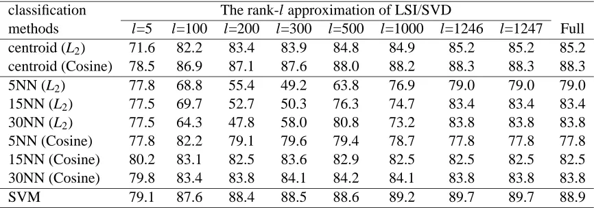
classification The rank-l approximation of LSI/SVD

methods l=5 l=100 l=200 l=300 l=500 l=1000 l=1246 l=1247 Full centroid (L2) 71.6 82.2 83.4 83.9 84.8 84.9 85.2 85.2 85.2 centroid (Cosine) 78.5 86.9 87.1 87.6 88.0 88.2 88.3 88.3 88.3 5NN (L2) 77.8 68.8 55.4 49.2 63.8 76.9 79.0 79.0 79.0 15NN (L2) 77.5 69.7 52.7 50.3 76.3 74.7 83.4 83.4 83.4 30NN (L2) 77.5 64.3 47.8 58.0 80.8 73.2 83.8 83.8 83.8 5NN (Cosine) 77.8 82.2 79.1 79.6 79.4 78.7 77.8 77.8 77.8 15NN (Cosine) 80.2 83.1 82.5 83.6 82.9 82.5 82.5 82.5 82.5 30NN (Cosine) 79.8 83.4 83.8 84.1 84.2 84.1 83.8 83.8 83.8

SVM 79.1 87.6 88.4 88.5 88.6 89.2 89.7 89.7 88.9

Table 1: Text classification accuracy (%) using centroid-based classification, k-nearest neighbor classification, and SVMs, with LSI/SVD dimension reduction on the MEDLINE data set. The Euclidean norm (L2) and the cosine similarity measure (Cosine) were used for the centroid-based and kNN classification.

The first data set that we used was a subset of the MEDLINE database with 5 classes. Each class has 500 documents. The set was divided into 1250 training documents and 1250 test documents. After stemming and stoplist removal, the training set contains 22095 distinct terms. For this data, each document belongs to only one class, and we used the original form of the three classification algorithms without introducing the threshold.

The second data set was the “ModApte” split of the Reuter-21578 text collection. We only used 90 classes for which there is at least one training and one test example in each class. It contains 7769 training documents and 3019 test documents. The training set contains 11941 distinct terms after preprocessing with stoplist removal and stemming. The Reuter data set contains documents that belong to multiple classes, so the classification methods utilize thresholds.

We used a standard weight factor for each word stem:

φi(x) =

t filog(id fi)

κ , (13)

where t fi is the number of occurrences of term i in document x, id fi=n/d is the ratio between the total number of documents n and the number of documents d containing the term, andκis the normalization constant that makes_kφ_k2=1.

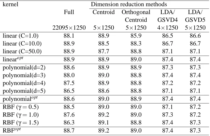
kernel Dimension reduction methods

Full Centroid Orthogonal LDA/ LDA/ Centroid GSVD4 GSVD5 22095_×1250 5_×1250 5_×1250 4_×1250 5_×1250

linear (C=1.0) 88.1 88.9 85.9 86.5 86.6

linear (C=10.0) 88.9 88.5 88.3 86.7 86.7

linear (C=50.0) 88.9 87.7 88.8 87.1 87.1

linearopt 88.9 88.9 89.0 87.4 87.4

polynomial(d=2) 88.6 88.9 88.9 87.3 87.3

polynomial(d=3) 88.0 89.0 88.8 87.4 87.4

polynomial(d=4) 87.5 88.9 88.8 87.2 87.2

polynomial(d=5) 86.5 88.6 88.8 87.1 87.1

polynomialopt 88.6 89.0 88.9 87.4 87.4

RBF (γ=0.5) 88.5 89.0 89.0 87.1 87.2 RBF (γ=1.0) 87.6 89.2 89.0 87.3 87.2 RBF (γ=1.5) 86.3 89.1 88.8 87.4 87.3

RBFopt 88.7 89.2 89.0 87.4 87.3

Table 2: Text classification accuracy (%) with different kernels in SVMs with and without dimen-sion reduction on the MEDLINE data set. The regularization parameter C for each case was optimized by numerical experiments. Dimension of each training term-document ma-trix is shown. LDA/GSVD4 and LDA/GSVD5 represent the results from LDA/GSVD where the reduced dimensions are 4 and 5, respectively.

of size 250. It is noteworthy that even with LSI, which makes no attempt to preserve the cluster structure upon dimension reduction, SVM classification achieves very consistent classification re-sults for reduced dimensions of 100 or greater, and the SVM accuracy exceeds that of the other classification methods.

Table 2 shows text classification accuracy (%) with different kernels in SVMs, with and without dimension reduction on the MEDLINE data set. Note that the linearopt values are optimal over all the values of the regularization parameter C that we tried, and the RBFopt values are optimal over all theγvalues we tried. This table shows that the prediction results in the reduced dimension are similar to those in the original full dimensional space, while achieving a significant reduction in time and space complexity. In the reduced space obtained by the Orthogonal Centroid dimension reduction algorithm, the classification accuracy is insensitive to the choice of the kernel. Thus, we can choose the linear kernel in this case instead of the computationally more expensive polynomial or RBF kernel.

classification Dimension reduction methods methods Full Centroid Orthogonal LDA/ LDA/

Centroid GSVD4 GSVD5 22095_×1250 5_×1250 5_×1250 4_×1250 5_×1250

centroid (L2) 85.2 88.0 85.2 88.7 88.7

centroid (Cosine) 88.3 88.0 88.3 83.9 83.9

5NN (L2) 79.0 88.4 88.6 81.5 86.6

15NN (L2) 83.4 88.3 87.8 88.7 88.6

30NN (L2) 83.8 88.8 88.5 88.7 88.5

5NN (Cosine) 77.8 88.6 88.2 83.8 84.1

15NN (Cosine) 82.5 88.2 88.5 83.8 84.1

30NN (Cosine) 83.8 88.3 88.6 83.8 84.1

SVM 88.9 89.2 89.0 87.4 87.4

Table 3: Text classification accuracy (%) using centroid-based classification, k-nearest neighbor classification, and SVMs, with and without dimension reduction on the MEDLINE data set. The Euclidean norm (L2) and the cosine similarity measure (Cosine) were used for centroid-based and kNN classification.

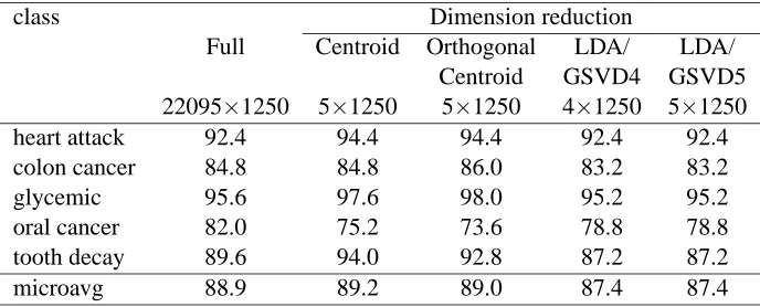
class Dimension reduction

Full Centroid Orthogonal LDA/ LDA/ Centroid GSVD4 GSVD5 22095_×1250 5_×1250 5_×1250 4_×1250 5_×1250

heart attack 92.4 94.4 94.4 92.4 92.4

colon cancer 84.8 84.8 86.0 83.2 83.2

glycemic 95.6 97.6 98.0 95.2 95.2

oral cancer 82.0 75.2 73.6 78.8 78.8

tooth decay 89.6 94.0 92.8 87.2 87.2

microavg 88.9 89.2 89.0 87.4 87.4

Table 4: Text classification accuracy (%) of the 5 classes and the microaveraged performance over all 5 classes on the MEDLINE data set. All results are from SVMs using optimal kernels.

the full dimensional space tend to be transformed to a very tight cluster or even to a single point in the reduced space, since the LDA/GSVD algorithm tends to minimize the trace of the within cluster scatter. This seems to make it difficult for SVMs to find a binary classifier with low generalization error.

Table 4 shows text classification accuracy for the 5 classes using SVMs with and without dimen-sion reduction methods on the MEDLINE data set. The colon cancer and oral cancer documents were relatively hard to classify correctly.

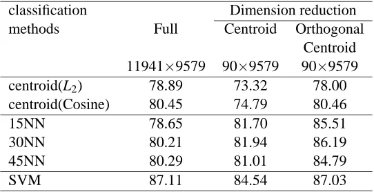
classification Dimension reduction methods Full Centroid Orthogonal

Centroid 11941_×9579 90_×9579 90_×9579 centroid(L2) 78.89 73.32 78.00 centroid(Cosine) 80.45 74.79 80.46

15NN 78.65 81.70 85.51

30NN 80.21 81.94 86.19

45NN 80.29 81.01 84.79

SVM 87.11 84.54 87.03

Table 5: Comparison of micro-averaged F1 scores for 3 different classification methods with and without dimension reduction on the REUTERS data set. The Euclidean norm (L2) and the cosine similarity measure (Cosine) were used for the centroid-based classification. The cosine similarity measure was used for the kNN classification. The dimension of the full training term-document matrix is 11941_×9579 and that of the reduced matrix is 90_×9579.

could handle relatively large matrices using a sparse matrix representation and sparse QR decom-position in the Centroid and Orthogonal Centroid dimension reduction methods, results for the LDA/GSVD dimension reduction method are not reported, since we ran out of memory while com-puting the GSVD. For this data set, we built a series of threshold-based classifiers, optimizing the thresholds to capture the multiple class membership. All class specific thresholds (θkNN_j ,θc_j,θSV M_j ) are determined by numerical experiments. Though we obtained precision/recall break even points by optimizing the thresholds, we report values of the F1measure (26) which is defined as

F1= 2r p

r+p, (14)

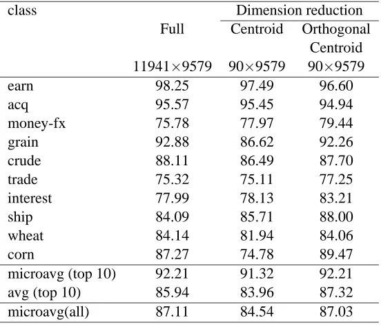
where r is recall and p is precision for a binary classification. Table 5 shows that the effectiveness of classification was preserved for the Orthogonal Centroid dimension reduction algorithm, while it became worse for the Centroid dimension reduction algorithm. This is due to a property of the Cen-troid algorithm that the cenCen-troids of the full space are projected to the columns of the identity matrix in the reduced space. This orthogonality between the centroids may make it difficult to represent the multiclass membership of a document by separating closely related classes after dimension reduc-tion. The pattern of prediction measure F1for each class is also preserved by Orthogonal Centroid in Table 6. The macro-averaged F1and micro-averaged F1for the 10 most frequent classes are also presented.

6. Conclusion and Discussion

class Dimension reduction Full Centroid Orthogonal

Centroid 11941_×9579 90_×9579 90_×9579

earn 98.25 97.49 96.60

acq 95.57 95.45 94.94

money-fx 75.78 77.97 79.44

grain 92.88 86.62 92.26

crude 88.11 86.49 87.70

trade 75.32 75.11 77.25

interest 77.99 78.13 83.21

ship 84.09 85.71 88.00

wheat 84.14 81.94 84.06

corn 87.27 74.78 89.47

microavg (top 10) 92.21 91.32 92.21 avg (top 10) 85.94 83.96 87.32 microavg(all) 87.11 84.54 87.03

Table 6: F1 scores of the 10 most frequent classes and micro-averaged performance over all 90 classes on the REUTERS data set. All results are from SVMs using optimal kernels. The dimension of the full training term-document matrix is 11941_×9579 and that of the reduced matrix is 90_×9579.

SVMs, kNN, and centroid-based classification. For the three cluster-preserving methods, the re-sults show surprisingly high prediction accuracy, which is essentially the same as in the original full space, even with very dramatic dimension reduction. They justify dimension reduction as a worthwhile preprocessing stage for achieving high efficiency and effectiveness. Especially for kNN classification, the savings in computational complexity in classification after dimension reduction are significant. In the case of SVM the savings are also clear, since the distance between two pairs of input data points need to be computed repeatedly with and without the use of the kernel function, and the vectors become significantly shorter with dimension reduction.

The better prediction accuracy using SVMs is due to low generalization error by maximizing the margin, and the capability to handle non-linearity by kernel choice. Although most classes of the Reuters-21578 data set are linearly separable (13), there seems to be some level of non-linearity. For non-linearly separable data, SVMs with appropriate nonlinear kernel functions would work as a better classifier. Another way to handle non-linearly separable data is to apply nonlinear extensions of the dimension reduction methods, including those presented in (18; 19). All of the dimension reduction methods presented here can also be applied to visualize the higher dimensional structure by reducing the dimension to 2- or 3-dimensional space.

We conclude that dramatic dimension reduction of text documents can be achieved, without sacrificing classification accuracy. For the document sets we tested, the Orthogonal Centroid method did particularly well at preserving the cluster structure from the full dimensional representation. That is, the prediction accuracies for Orthogonal Centroid rival those of the full space, even though the dimension is reduced to the number of clusters. The savings in computational complexity are significant using either kNN classification or SVM.

Acknowledgments

This material is based upon work supported by the National Science Foundation Grant No. CCR-0204109. Any opinions, findings and conclusions or recommendations expressed in this material are those of the authors and do not necessarily reflect the views of the National Science Foundation (NSF). The authors would also like to thank University of Minnesota Supercomputing Institute (MSI) for providing the computing facilities.

References

[1] M. W. Berry, Z. Drmac, and E. R. Jessup. Matrices, vector spaces, and information retrieval.

SIAM Review, 41:335–362, 1999.

[2] M. W. Berry, S. T. Dumais, and G. W. O’Brien. Using linear algebra for intelligent information retrieval. SIAM Review, 37:573–595, 1995.

[3] M. W. Berry and R. D. Fierro. Low-rank orthogonal decompositions for information retrieval applications. Numerical Linear Algebra with Applications, 3(4):301–327, 1996.

[4] ˚A. Bj¨orck. Numerical Methods for Least Square Problems. SIAM, Philadelphia, PA, 1996.

[5] N. Cristianini and J. Shawe-Taylor. Support Vector Machines and Other Kernel-based

Learn-ing Methods. Cambridge University Press, 2000.

[6] S. Deerwester, S.T. Dumais, G.W. Furnas, T.K. Landauer, and R. Harshman. Indexing by latent semantic analysis. Journal of the Society for Information Science, 41:391-407, 1990.

[7] K. Fukunaga, Introduction to Statistical Pattern Recognition, Second ed., Academic Press, 1990.

[9] M. Heiler. Optimization Criteria and Learning Algorithms for Large Margin Classifiers. Diploma Thesis, University of Mannheim., 2002.

[10] P. Howland, M. Jeon, and H. Park. Structure Preserving Dimension Reduction for Clustered Text Data based on the Generalized Singular Value Decomposition. SIAM Journal of Matrix

Analysis and Applications, 25(1):165–179, 2003.

[11] P. Howland and H. Park. Generalizing discriminant analysis using the generalized singular value decomposition, IEEE Transactions on Pattern Analysis and Machine Intelligence, 26(8): 995-1006, 2004.

[12] M. Jeon, H. Park, and J. B. Rosen. Dimensional reduction based on centroids and least squares for efficient processing of text data. In Proceedings for the First SIAM International Workshop

on Text Mining. Chicago, IL, 2001.

[13] T. Joachims. Text categorization with support vector machines: Learning with many relevant features. In Proceedings of the European Conference on Machine Learning, pages 137–142, Berlin, 1998.

[14] H. Lodhi, N. Cristianini, J. Shawe-Taylor, and C. Watkins. Text classification using string kernels. Advances in Neural Information Processing Systems, 13:563–569, 2000.

[15] C. C. Paige and M. A. Saunders, Towards a generalized singular value decomposition, SIAM

Journal of Numerical Analysis, 18, pp. 398–405, 1981.

[16] H. Park, M. Jeon, and J. B. Rosen. Lower dimensional representation of text data based on centroids and least squares, BIT Numerical Mathematics, 42(2):1–22, 2003.

[17] H. Park and L. Eld´en. Downdating the rank-revealing URV decomposition. SIAM Journal of

Matrix Analysis and Applications, 16, pp. 138–155, 1995.

[18] C. Park and H. Park. Nonlinear feature extraction based on centroids and kernel functions.

Pattern Recognition, to appear.

[19] C. Park and H. Park. Kernel discriminant analysis based on the generalized singular value decomposition. Technical report 03-017, Department of Computer Science and Engineering, University of Minnesota, 2003.

[20] G. Salton, The SMART Retrieval System, Prentice Hall, 1971.

[21] G. Salton and M. J. McGill, Introduction to Modern Information Retrieval, McGraw-Hill, 1983.

[22] G. W. Stewart. An updating algorithm for subspace tracking. IEEE Transactions on Signal

Processing, 40:1535–1541, 1992.

[23] G. W. Stewart. Updating URV decompositions in parallel. Parallel Computing, 20(2):151– 172, 1994.

[24] M. Stewart and P. Van Dooren. Updating a generalized URV decomposition. SIAM Journal of

[25] S. Theodoridis and K. Koutroumbas, Pattern Recognition, Academic Press, 1999.

[26] C. J. van Rijsbergen. Information Retrieval. Butterworths, London, 1979.

[27] V. Vapnik. The Nature of Statistical Learning Theory. Springer-Verlag, New York, 1995.

[28] V. Vapnik. Statistical Learning Theory. John Wiley & Sons, New York, 1998.

[29] Y. Yang and X. Liu. A re-examination of text categorization methods. In 22nd Annual