Learning Probabilistic Models: An Expected Utility
Maximization Approach
Craig Friedman CRAIG [email protected]
Sven Sandow SVEN [email protected]
Standard & Poor’s Risk Solutions Group 55 Water Street New York, NY 10041
Editors: David Maxwell Chickering
Abstract
We consider the problem of learning a probabilistic model from the viewpoint of an expected util-ity maximizing decision maker/investor who would use the model to make decisions (bets), which result in well defined payoffs. In our new approach, we seek good out-of-sample model perfor-mance by considering a one-parameter family of Pareto optimal models, which we define in terms of consistency with the training data and consistency with a prior (benchmark) model. We measure the former by means of the large-sample distribution of a vector of sample-averaged features, and the latter by means of a generalized relative entropy. We express each Pareto optimal model as the solution of a strictly convex optimization problem and its strictly concave (and tractable) dual. Each dual problem is a regularized maximization of expected utility over a well-defined family of functions. Each Pareto optimal model is robust: maximizing worst-case outperformance relative to the benchmark model. Finally, we select the Pareto optimal model with maximum (out-of-sample) expected utility. We show that our method reduces to the minimum relative entropy method if and only if the utility function is a member of a three-parameter logarithmic family.
Keywords: Learning Probabilistic Models, Expected Utility, Relative Entropy, Pareto Optimality,
Robustness
1. Introduction
Cover and Thomas, 1991 for a discussion of the horse race). In particular, we monetize the decision consequences by assuming that there is a market with payoffs associated with each state (the horse race). The assumption of a rational investor who bets on horses allows us to relate the model user’s decisions and their consequences to the model itself; as we shall see, this assumption leads to tractable models. Our approach combines ideas from maximum entropy modeling and utility theory.
Maximum entropy inference, introduced by Jaynes (1957, 1982, 1984) in the context of sta-tistical physics, has been successfully applied to image processing (see, for example, Wu, 1997, or Gull and Daniell, 1978) as well as to a wide range of problems in biology (see, for example, Burnham and Anderson, 2002), finance (see, for example, Avellaneda, 1998, Avellaneda et al., 1997, Samperi, 1997, Gulko, 2002 and Frittelli, 2000) and economics (see, for example, Golan et al., 1996). The basic idea of the maximum entropy approach is that one chooses a model that maximizes uncertainty, or, more generally, minimizes the information-theoretic (Kullback-Leibler) distance to a prior, while ensuring that important features of the data are reproduced. In many ap-plications, in order to avoid overfitting, one has to allow for some error in the calibration of the model-expected feature values to the expected feature values under the empirical measure (see, for example, Daniell, 1991, Skilling, 1991, Wu, 1997, Chen and Rosenfeld, 1999, or Lebanon and Lafferty, 2001).
In order to evaluate a model in terms of the decision consequences of a rational decision maker who believes the model, we need to first relate the rational decisions to the model and then evaluate the consequences of these decisions. For both of these purposes, we employ a utility function, a well established concept in economics (see, for example, Neumann and Morgenstern, 1944, or Luenberger, 1998). One can show that, under some additional plausible assumptions, a decision maker has a well defined utility function if he has preferences between the possible states of the world and probability weighted combinations of these states. It follows from the axioms of utility theory that a rational decision maker acts to maximize his expected utility based on the model he believes; his decisions are uniquely (and explicitly) determined by his model. Utility theory also dictates that the consequences of these decisions should be evaluated by means of the expected utility they lead to.
Friedman and Sandow (2003a) consider the performance of probabilistic models from the point of view of an expected utility maximizing investor who bets on horses. In order to evaluate a particular model, we assume that there is an investor who believes the model. This investor places bets in a horse race so as to maximize his expected utility according to his beliefs, i.e., the investor bets so as to maximize the expectation of his utility under the model probability measure. We then measure the success of the investor’s investment strategy in terms of the average utility the strategy provides on an out-of-sample data set. An investor who has a highly accurate model will be able to choose a sound investment strategy, while an investor with a less accurate model will sometimes overbet or underbet, and consequently, be less successful in the long run. Therefore, the success of the investor’s strategy, as measured by the utility averaged over a test sample, is a measure of the quality of the model on which the investor bases his strategy. This measure was used to evaluate probabilistic models.
which is different from existing approaches, is based on the idea that one can achieve good out-of-sample model performance (as measured by expected utility under the model-optimal strategy) by considering models on an efficient frontier (Pareto optimal models), which we define in terms of consistency with the training data and consistency with a prior (benchmark) model. We measure the former by means of the large-sample distribution of a vector of sample-averaged features, and the latter by means of the generalized relative entropy introduced by Friedman and Sandow (2003a). This generalized relative entropy is essentially the same as the one independently introduced by Gr¨unwald and Dawid (2002). The models on the efficient frontier, each of which can be obtained by solving a convex optimization problem (see Problems 2 and 8) form a single-parameter family. We show that each Pareto optimal model is robust in the sense that, for its level of consistency with the data, the model maximizes the worst-case outperformance relative to the benchmark model (see Section 2.2.5 and Appendix A). For each level of consistency with the data, we derive the dual problem (see Problems 3, 4 and 9), which has a Pareto optimal measure as its solution; this dual problem, which is new for non-logarithmic utility functions, amounts to the maximization of expected utility with a regularization penalty over a well-defined family of functions. We rank the models on the efficient frontier by computing their expected utilities on a hold-out sample, and select the model with maximum estimated expected utility. For ease of exposition, we consider only one hold-out sample; our procedure can be modified for k−fold cross validation.
Our economic paradigm, in general, requires the specification of the payoff structure of the horse race. This requirement imposes an additional encumbrance on the model-builder. However, we show that the optimization problems that follow from our paradigm are independent of the payoffs if and only if the investor’s utility function is in a three-parameter logarithmic family (see Theorem 3). This logarithmic family is rich enough to describe a wide range of risk aversions, and it can be used to well-approximate (under reasonable conditions) non-logarithmic utility functions (see Friedman and Sandow, 2003a); it is therefore applicable to many practical problems. In the case of a utility function from this logarithmic family, our method leads to a regularized relative entropy minimization similar to the ones by Daniell (1991), Skilling (1991), Wu (1997), or Lebanon and Lafferty (2001) (see Corollary 1). This means that our approach provides new motivation of this regularized relative entropy minimization. It is well known that the relative entropy can be related to the expected utility of an investor with a logarithmic utility (of the form U(z) =log(z)) who bets optimally in a horse race (see, for example, Cover and Thomas, 1991). Our result, however, is more general since we allow the investor’s utility to be any member of the three-parameter family of logarithmic functions given by U(z) =γ1log(z+γ) +γ2.
Some of our discussion, such as the definition and robustness of the Pareto optimal measures (See Appendix A) and the formulation of the primal problems (see Sections 2.2 and 3.2), can be developed in a more general setting than the horse race. However, our dual problem formulation (see Sections 2.3 and 3.3), depends on the horse race setting. To keep things as simple as possible, we have confined our discussion to the horse race setting.
2. Discrete Probability Models
In this section, we describe our modeling paradigm in the simplest context: discrete probabilities.
2.1 Preliminaries
This section sets the stage for our modeling approach for the case of discrete probabilities. The ideas outlined below are explained in more detail in Section 2 in Friedman and Sandow (2003a).
We seek a probabilistic model for the discrete random variable Y , which can take any of the m values y1,...,ym. For later use we define the following three probability measures:
Definition 1
py = true (unknown) probability that Y=y,
˜
py = empirical probability that Y=y, qy = model probability that Y=y.
The true probabilities, p= (p1,...,pm)T, are unknown, but we assume their existence; the em-pirical probabilities, ˜p = (p˜1,...,p˜m)T, are known from the data, and the model probabilities, q= (q1,...,qm)T, are the ones we are trying to find. We define the probability simplex
Q={q : q≥0,
∑
y
qy=1}.
We identify the probabilistic problem with the horse race (see , for example, Cover and Thomas, 1991, Chapter 6; Cover and Thomas discuss the horse race from the point of view of an investor with logarithmic utility).
Definition 2 A horse race is a market characterized by the discrete random variable Y with m possible states, in which an investor can place a bet that Y =y, which pays
O
y>0 for each dollar wagered if Y =y, and 0, otherwise.1We consider a decision maker/investor2 who places bets on horses; we assume that our investor allocates by to the event Y =y, where
∑
y
by=1. (1)
We note that Equation 1 corresponds to the assumption that the investor allocates all his wealth to bets on the horses, without cash borrowing or lending. This setting does not represent the most general financial market.
In order to quantify the benefits of a model q to an expected utility-maximizing investor, we consider the investor’s utility function, U , and assume that it is
(i) strictly concave,
1. The investor does not get his dollar back in addition to the payoff,Oy. This horse race definition is general enough to
allow for situations where the investor loses with certainty.
(ii) twice differentiable, and
(iii) strictly monotone increasing.
We note that many popular utility functions (for example, the logarithmic, exponential and power utilities (see Luenberger, 1998)) are consistent with these conditions. It is possible to develop the ideas in this paper under more relaxed assumptions.
Our investor allocates his assets so as to maximize his expected utility according to his beliefs, i.e., the investor allocates so as to maximize the expectation of his utility under the model probability measure. This means that our investor allocates according to
b∗(q) =arg max
{b:∑yby=1}
∑
yqyU(by
O
y). (2)It has been shown (see Theorem 1 from Friedman and Sandow, 2003a) that
b∗y(q) = 1
O
y(U0)−1
λ
qy
O
y
, (3)
whereλis the solution of the following equation:
∑
y
1
O
y (U0)−1λ
qy
O
y
=1 , (4)
if the solution of Equation 4 exists, which we assume to be the case here:
Assumption 1 There exists a solution to Equation 4.
We note that there does not always exist a solution to Equation 4, however, there exists a solution for many common utilities, for example the logarithmic, power, exponential and quadratic utilities (see Corollary 1, Appendix B of Friedman and Sandow, 2003a).
Equipped with above tools, we can formulate our modeling objective:
Objective:
Find arg max
q∈QEp[U(b
∗(q),
O
)], (5)where, slightly abusing notation,
Ep[U(b∗(q),
O
)] =∑
ypyU(b∗y(q)
O
y).Thus, it is our objective to find the model that maximizes the true expectation of the utility of an investor who bets according to the model.
Since we don’t know the true model, p, we cannot compute the p−expectation in Equation 5 exactly. Therefore, we approximate it by a sample average; in order to construct models that don’t overfit, we approximate the p−expectation in Equation 5 by an average over a test sample:
Ep[U(b∗(q),
O
)]≈Ep[˜U(b∗(q),O
)],where ˜p is the empirical measure of the test sample, which is different from the sample the model
over an arbitrary family of models. However, one can easily (numerically) maximize Ep[U(b˜ ∗(q),
O
)]over a one-parameter family of models. This is the approach we will take. In Sections 2.2 and 2.3 we will describe how one can construct a one-parameter family of candidate models based on the idea of an efficient frontier, which we define in terms of consistency with the training data and con-sistency with a prior distribution. We shall see that the construction of the candidate models involves a regularized in-sample expected utility maximization, and that each candidate model is robust in the sense that, for its level of consistency with the data, it maximizes the worst case outperformance relative to the benchmark model. This is another rationale for our choice of candidate models.
For our approach we will make use of the concept of generalized relative entropy, which was introduced in Friedman and Sandow (2003a) (Section 2.2). A very similar generalization of the relative entropy was independently introduced by Gr¨unwald and Dawid (2002). The approach in Gr¨unwald and Dawid (2002) is based on the idea of expected loss, and is therefore closely related to the approach in Friedman and Sandow (2003a), in which the utility function of an investor who bets (utility-optimally) on horses leads to an expected utility that can be viewed as the negative of an expected loss. Unlike Gr¨unwald and Dawid (2002), however, Friedman and Sandow (2003a) explicitely link the decision-maker’s/investor’s action/investment-strategy to the probabilities he assigns to the states of the world. In Friedman and Sandow (2003a), the generalized relative entropy between the measures q and q0was defined as
DU,O(q||q0) =
∑
yqyU(b∗y(q)
O
y)−∑
yqyU(b∗y(q0)
O
y) (6)It can be interpreted as the loss in expected utility experienced by an investor who bets according to model q0when q is the true probability measure. It has been shown (see Friedman and Sandow, 2003a, Theorem 2) that DU,O(q||q0)is a strictly convex function of q and that DU,O(q||q0)≥0 with
equality if and only if q=q0. We note that for U(W) =γ1log(W+γ) +γ2, DU,O reduces to the
Kullback-Leibler relative entropy, up to a constant factor (see Theorem 3 in Section 2.5, below).
2.2 Modeling Approach
We consider the tradeoff between consistency with the data and consistency with the investor’s prior beliefs (as encoded in the prior measure, q0). This approach is similar to others; see, for example, Lebanon and Lafferty (2001) or Wu (1997). However, we strive to formulate our problem(s) in economically meaningful ways. Given models equally consistent with the investor’s prior beliefs, we assume that the investor prefers a model that is more consistent with the data; given models equally consistent with the data, we assume that the investor prefers a model that is more consistent with the investor’s prior beliefs. We also show that these assumptions lead to measures which are robust, in the sense that they maximize a worst-case relative outperformance over the benchmark model. We make all of this precise below.
2.2.1 CONSISTENCY WITH THEDATA
For a model measure q∈Q, let µdata(q) denote the investor’s measure of the consistency of q with the data; this consistency is expressed in terms of expectations of the feature vector, f(y) = (f1(y),...,fJ(y))T ∈RJ where each feature,3 f
j, is a mapping from R to R. We make the following
assumption:
Assumption 2 The investor measures the consistency,4 µdata(q), of the model q∈Q with the data as a strictly monotone decreasing function of the large sample probability density of the sample feature means, evaluated at the model q feature expectations, Eq[f].
It is possible (for small sample sets, for example) to develop the theory under more general assump-tions, by considering more general families of convex level sets.
To elaborate, for a fixed measure q∈Q, the model feature mean, Eq[fj], is a deterministic quantity depending on q. The sample mean of fj, however, depends on the sample set and is
therefore a random variable, φj. The quantity Ep[˜ fj] is therefore an observation of the random
variable φj. By the Central Limit Theorem, for a large number of observations, N, the random
vector φ= (φ1,...,φJ)T is approximately normally distributed with mean Ep[˜ f] and covariance
matrix N1Σ, where Σ is the empirical feature covariance matrix. Therefore, for a given measure
q∈Q, the probability density for the random variableφ, evaluated at Eq[f]is (approximately) given by
pc(c)≡ pd f(φ)|φ=E
q[fj]= (2π)
−1 2JN
1 2|Σ|−
1 2e−
N 2c
TΣ−1c
, (7)
where
c= (c1,...,cJ)T
and
cj=Eq[fj]−Ep[˜ fj]. (8)
We note that though we have used the Central Limit Theorem to motivate our assumption, we have not made any assumption on the probability distribution of the measures q∈Q. Our
assump-tion allows us to parameterize the degree of consistency of a measure q with the data. Equally consistent measures, q, lie on the same level set of the function µdata(q). We parameterize the nested family of sets, consisting of points q∈Q that are equally consistent with the data.
Note that, by construction, µdata(q)is invariant with respect to translations and rotations of the feature vectors. James Huang (2003) first pointed this out to the authors.
2.2.2 CONSISTENCY WITH THEPRIORMEASURE
To quantify consistency of the model, q∈Q, with the investor’s prior beliefs, we make use of the
generalized entropy DU,O(q||q0), where U is the investor’s utility function and
O
is the set of oddsratios.
Assumption 3 The investor measures the consistency, µprior(q), of the model q∈Q with the prior, q0, by using some strictly monotone increasing function of the generalized relative entropy DU,O(q||q0).
More precisely, low µ values are associated with highly consistent models and high µ values are associated with less consistent models. We shall see in Section 2.3 that generalized relative entropy is an appropriate measure of consistency, as it leads to models which asymptotically maximize expected utility.
2.2.3 PARETOOPTIMAL MEASURES
To characterize the measures q∗∈Q which are optimal (in a sense to be made precise), we define dominance, Pareto optimal probability measures, the set of achievable measures, and the efficient frontier. These notions are from vector optimization theory (see, for example, Boyd and
Vanden-berghe, 2001) and portfolio theory (see, for example, Luenberger, 1998).
Definition 3 q1∈Q dominates q2∈Q with respect to µdataand µpriorif (i)
(µdata(q1),µprior(q1))6= (µdata(q2),µprior(q2)) and
(ii)
µdata(q1)≤µdata(q2) and
µprior(q1)≤µprior(q2).
Observe that q1∈Q dominates q2∈Q with respect to µdata and µprior if and only if q1 ∈Q
dominates q2 ∈Q with respect to tdata(µdata) and tprior(µprior), where tdata and tprior are strictly monotone increasing functions. Therefore, it follows from Equation 7 and Assumptions 2 and 3 that, without loss of generality, we may continue our discussion with5
µdata(q) =α(q)≡NcTΣ−1c≥0 (9) and
µprior(q) =DU,O(q||q0).
This choice is convenient as it leads to numerically tractable convex optimization problems (see Sec-tion 2.3, below). We note thatα(q)is the Mahalanobis distance. For a definition of the Mahalanobis distance and its properties, see, for example, Kullback (1997), p. 190.
Definition 4 A model, q∗∈Q, is Pareto optimal if and only if no measure q∈Q dominates q∗with respect to µdata(q) =α(q) and µprior(q) =DU,O(q||q0). The efficient frontier is the set of Pareto
optimal measures.
We note that for any Pareto optimal measure q∗∈Q,
α(q)≤α(q∗)implies that D
U,O(q||q0)≥DU,O(q∗||q0) (10)
for all q∈Q.
The Pareto optimal measures are contained in the achievable set,
A
, which is defined as follows:Definition 5 The achievable set,
A
, is given byA
={(α,D)|α(q)≤αand DU,O(q||q0)≤D for some q∈Q} ⊂R2.We slightly abuse notation: we sometimes useαand D to denote functions, and at other times we use the same symbols to denote real values; our intentions should be clear from the context.
By Equations 8 and 9, measures q that are equally consistent with the data lie on the same level set of the function
α(q) =N(Eq[f]−Ep[˜ f])TΣ−1(Eq[f]−Ep[˜ f]). (11)
We parameterize the nested family of sets, consisting of points q∈Q that are equally consistent with
the data, by Equation 11. We note that Σ−1 is a nonnegative definite matrix, soα(q) is a convex function of q.
The achievable set,
A
, is convex. To see this, recall that α(q) and DU,O(q||q0) are convexfunctions of q (see the remark following Equation 11 for the convexity of α(q); see Friedman and Sandow (2003a), Theorem 2 for the strict convexity of DU,O(q||q0)).
A
is convex by theconvexity of α(q) and DU,O(q||q0) (see, for example, Boyd and Vandenberghe, 2001, Section
4.7). The convexity of the achievable set follows from the particular choice µdata(q) =α(q) and
µprior(q) =DU,O(q||q0).
We may visualize the achievable set,
A
, and the efficient frontier as displayed in Figure 1, which also incorporates the following lemma.Lemma 1 If q∗is a Pareto optimal measure, then
(i) α(q∗)≤αmax, where
αmax=N(Eq0[f]−Ep[˜ f])TΣ−1(Eq0[f]−Ep[˜ f]). (12)
(ii) (α(q∗),DU,O(q∗||q0))lies on the lower D−boundary of
A
.Proof: (i) For the measure q0, we haveα(q0) =αmaxand D=DU,O(q0||q0) =0. Ifα(q)>αmax,
then q cannot be identical to q0, so DU,O(q||q0)>0, so q is dominated by q0and cannot be efficient.
(ii) follows directly from Equation 10.
We shall make use of the preceding lemma when we formulate our optimization problem. We make the following assumption, which serves as one of our guiding principles.
Assumption 4 The investor selects a measure on the efficient frontier.
Thus, given a set of measures equally consistent with the prior, our investor prefers measures that are more consistent with the data, and, given a set of measures equally consistent with the data, he prefers measures that are more consistent with the prior. He makes no assumptions about the precedence of these two preferences. We shall see (in Section 2.2.5) that every Pareto optimal measure is robust in the sense that it maximizes, over all measures, the worst-case (over measures equally consistent with the data) relative outperformance of the model over the benchmark model.
2.2.4 CONVEXOPTIMIZATION PROBLEM
We seek the set of Pareto optimal measures. That is, motivated by Lemma 1, for all q∈Q with α(q) =α, we seek all solutions of the following problem, asαranges from 0 toαmax, whereαmax
is defined in Equation 12.
Problem 1 (Initial Problem, Givenα,0≤α≤αmax)
Find arg inf
q∈(R+)m,c∈RJDU,O(q||q
0) (13)
under the constraints 1 =
∑
y
qy (14)
and NcTΣ−1c = α (15)
where cj = Eq[fj]−Ep[˜ fj] . (16)
Problem 1 is not a standard convex optimization problem (see, for example, Berkovitz, 2002), since Equation 15 is a non-affine equality constraint. However, we formulate a different (strictly convex optimization) problem, which, as we shall show, has the same solutions:
Problem 2 (Initial Strictly Convex Problem, Givenα,0≤α≤αmax)
Find arg min
q∈(R+)m,c∈RJDU,O(q||q
0) (17)
under the constraints 1 =
∑
y
qy (18)
and NcTΣ−1c ≤ α (19)
where cj = Eq[fj]−Ep[˜ fj] . (20)
Proof: See Appendix B.
In order to visualize the solutions to Problem 2, we define
Sα={q : NcTΣ−1c=α,q∈Qc}, (21)
where
Qc={q : q≥0,
∑
y
qy=1,
∑
y
qyfj(y) =cj+Ep[˜ fj],j=1,...,J}.
By solving Problem 2, for each α, we generate a one-parameter family of candidate models,
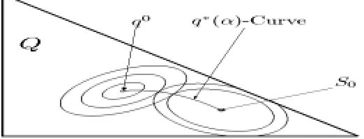
q∗(α), indexed by α. We can visualize these models as the points of tangency (on the probabil-ity simplex, Q) of the nested surfaces of the families Sα and the level sets of DU,O(q||q0) (see
Figure 2). Each candidate model, q∗(α), is a solution of Problem 2; accordingly, each point
(α,DU,O(q∗(α)||q0)) is a point on the efficient frontier (see Figure 1), and the efficient frontier consists of all points of the form(α,DU,O(q∗(α)||q0)), asαranges from(0,αmax).
Figure 2: The sets Sα (see Equation 21), centered at S0, the q∗(α)-curve, and the level sets of DU,O(q||q0), centered at q0, on the probability simplex Q
2.2.5 ROBUSTNESS OF THEPARETOOPTIMALMEASURES
We can measure the quality of a model q by the relative outperformance of the model over the benchmark model,6 q0: the gain in expected (under the true measure) utility experienced by an in-vestor who invests optimally according to the model relative to an inin-vestor who invests optimally according to the benchmark model q0(see Friedman and Sandow, 2003a). That is, the relative out-performance is given by Ep0
U(b∗(q),
O
)−U(b∗(q0),O
), where p0 is a potential true probabilitymeasure. It follows from the fact that the Pareto optimal measures are solutions of Problem 2 and from Theorem 5 (in Appendix A) that every Pareto optimal measure, q∗(α), is robust in the follow-ing sense: it maximizes, over all measures, the worst-case (with respect to potential true measures
6. Here, we look at the prior, q0, from a slightly different perspective; in this context, we view q0as a model against
equally consistent with the data) relative outperformance of the model over the benchmark model, i.e.,
q∗(α) =arg max
q∈Qpmin0∈Sα
Ep0[U(b∗(q),
O
)]−Ep0U(b∗(q0),O
) .2.2.6 CHOOSING AMEASURE ON THEEFFICIENTFRONTIER
According to our paradigm, the best candidate model lies on a one-parameter efficient frontier. In order to choose the best candidate model from this one-parameter family, we make the following assumption.
Assumption 5 The investor choosesαso as to maximize his expected utility on an out-of-sample data set.
Thus, given a utility function, U , odds ratios,
O
, and a prior belief, q0, Assumptions 1 to 5 lead to a method for finding a probability measureq∗∗ = q∗(α∗),
with α∗ = arg max
α Ep[˜U(b∗(q∗(α)),
O
)],where ˜p is the empirical measure of the test set. In our method, the relative importance of the data
and the prior is determined by the out-of-sample performance (expected utility) of the model.
2.2.7 INFORMALCOMMENT: PRACTICALBOUND FORα
In practice, given a confidence level, l, under Assumption 2, we can search over the range,
α∈(0,αsearch),
where
αsearch=min(αl,αmax)
and
αl = (cd fχ2 J)
−1(l)
(see, for example, Davidson and MacKinnon, 1993 or Wu, 1997). That is, we search until
(i) we are 100·l% confident that the true value of c is within the region NcTΣ−1c≤α,
(ii) the region NcTΣ−1c≤αincludes q0and q∗is insensitive to further increasing the value ofα.
2.3 Dual Problem
We have shown in Section 2.2 that, in order to find the Pareto optimal model, q∗, for a givenα, we have to solve Problem 2. As we have seen, this problem is strictly convex. Convex problems are known to have so called dual problems.
We show in Appendix C that the dual of Problem 2 can be formulated as:
Problem 3 (Easily Interpreted Version of Dual Problem, Givenα)
Findβ∗ = arg max
β h(β) (22)
with h(β) =
∑
y
˜
pyU(b∗y(q∗)
O
y) −r
αβTΣβ
N , (23)
where b∗y(q∗) = 1
O
y(U0)−1 λ ∗
q∗y
O
y!
(24)
and q∗y = λ
∗
O
yU0(U−1(Gy(q0,β,µ∗))), (25)
with Gy(q0,β,µ∗) = U(b∗
y(q0)
O
y) + βTf(y) − µ∗ , (26)where µ∗solves 1 =
∑
y
1
O
yU−1 Gy(q0,β,µ∗) , (27)
and λ∗ =
(
∑
y
1
O
yU0(U−1(Gy(q0,β,µ∗))))−1
. (28)
Equation 25 is often referred to as the connecting equation (see, for example, Lebanon and Lafferty, 2001).
We also show in Appendix C that an alternative formulation of the dual problem is the following:
Problem 4 (Easily Implemented Version of Dual Problem, Givenα)
Findβ∗ = arg max
β h(β) (29)
with h(β) = βTEp[˜ f] −µ∗ −
r
αβTΣβ
N , (30)
where µ∗solves 1 =
∑
y
1
O
yU−1 Gy(q0,β,µ∗) (31)
with Gy(q0,β,µ∗) = U(b∗y(q0)
O
y) + βTf(y) − µ∗ . (32) The optimal probability distribution is thenq∗y = λ
∗
O
yU0(U−1(Gy(q0,β∗,µ∗))) , (33)with λ∗ =
(
∑
y
1
O
yU0(U−1(Gy(q0,β∗,µ∗))))−1
We state the following theorem:
Theorem 1 Problems 2, 3 and 4 have the same unique solution, q∗y. Proof: see Appendix C.
Problems 3 and 4 are equivalent. Problem 4 is easier to implement and Problem 3 is easier to interpret. The first term in the objective function of Problem 3 is the utility (of the utility maximizing investor) averaged over the training sample. Thus, our dual problem is a regularized maximization of the training-sample averaged utility, where the utility function, U , is the utility function on which the generalized relative entropy DU,O(q||q0)depends.
The dual problems, Problems 3 and 4, are J-dimensional (J is the number of features), un-constrained, concave maximization problems (see Boyd and Vandenberghe, 2001, p. 159 for the concavity). The primal problem, Problem 2, on the other hand, is an m-dimensional (m is the num-ber of states) convex minimization with convex quadratic constraints. The dual problem, Problem 4, may be easier to solve than the primal problem, Problem 2, if m>J. In the more general context
discussed in section 3, the dual problem will always be easier to solve than the primal problem. We note that we can obtain the same α−parameterized family of solutions to Problems 3 and 4, if we allowαto vary over[0,∞), by dropping the square roots in Equations 23 and 30; we show that this is so in Appendix E.
2.3.1 ASYMPTOTIC OPTIMALITY
It follows from Equation 23 that
Theorem 2 As N→∞, to leading order, the optimal solution to Problem 2 maximizes (over the parametric family prescribed by the connecting equation, Equation 25) the expected utility for the investor.
2.3.2 EXAMPLE: A LOGARITHMIC FAMILY OF UTILITIES
We consider a utility of the form
U(z) = γ1log(z+γ) +γ2 ,γ>−
1
∑yOy1
,γ1>0 , (35)
(see Theorems 3 and 4 in Friedman and Sandow, 2003a). This logarithmic family is rich enough to describe a wide range of risk aversions; and it can be used to approximate non-logarithmic utility functions (see Friedman and Sandow, 2003a).
In Appendix D, we show that the dual problem is given by:
Problem 5 (Dual Problem for our Logarithmic Family of Utilities) Findβ∗ = arg max
β h(β)
with h(β) =
∑
y
˜
pylog q∗y −
s
α γ2 1
βTΣβ
N ,
where q∗y = 1
∑yq0yeβ
Tf(y) q
0 yeβ
Tf(y)
This problem is equivalent to a regularized maximum likelihood search, which is independent of the odds ratios,
O
; this is consistent with Section 2.5, where we show that the odds ratios drop out of the primal problem for this logarithmic family of utility functions.2.3.3 EXAMPLE: POWER UTILITY
We consider a utility of the form
U(z) = z 1−κ−1
1−κ . (36)
(see Section 2.1.1 in Friedman and Sandow, 2003a). In order to specify the dual problem for this utility, note that
U0(z) = z−κ, (37)
U−1(z) = [1+ (1−κ)z]1−κ1 (38)
and U0(U−1(z)) = [1+ (1−κ)z]1−κ−κ . (39)
One can show that
b∗(q) = (qy
O
y)1 κ
O
yB(q,O
)(40)
with B(q,
O
) =∑
y1
O
y(qy
O
y)κ1 , (41)(see Section 2.1.1 in Friedman and Sandow, 2003a). Using this equation, we can write Gy(q0,β,µ∗)
from Equation 26 as
Gy(q0,β,µ∗) = 1
1−κ "
(q0y
O
y)1−κκ(B(q0,
O
))1−κ! −1
#
+βTf(y) −µ∗ . (42)
Inserting Equations 38 and 42 into Equation 27 gives
1 =
∑
y
1
O
y"
(q0y
O
y)1−κ κ(B(q0,
O
))1−κ+ (1−κ)[βTf(y)−µ∗]
# 1 1−κ
, (43)
which is our condition for µ∗. Next we specify the condition Equation 28 forλ∗. We use Equations 39 and 42 to write Equation 28 as
λ∗ =
∑
y1
O
y"
(q0y
O
y)1−κ κ(B(q0,
O
))1−κ+ (1−κ)[βTf(y)−µ∗]
# κ 1−κ −1 . (44)
By means of Equations 25, 39 and 42 we obtain for the optimal probability distribution
q∗y = 1
O
y"
(q0y
O
y)1−κκ(B(q0,
O
))1−κ+ (1−κ)[βTf(y)−µ∗]
# κ 1−κ
. (45)
Problem 6 (Dual problem for power utility)
Findβ∗ = arg max
β h(β)
with h(β) = βTE ˜
p[f]− µ∗ −
r
αβTΣβ
N ,
where µ∗solves 1 =
∑
y
1
O
y"
(q0 y
O
y)1−κ κ
(B(q0,
O
))1−κ+ (1−κ)[βTf(y)−µ∗]
# 1 1−κ
with B(q0,
O
) =∑
y
1
O
y (q0y
O
y)1 κ .
The optimal probability distribution is then
q∗y = λ
∗
O
y"
(q0y
O
y)1−κκ(B(q0,
O
))1−κ+ (1−κ)[β∗Tf(y)−µ∗]
# κ 1−κ
with λ∗ =
∑
y1
O
y"
(q0y
O
y)1−κκ(B(q0,
O
))1−κ+ (1−κ)[β∗Tf(y)−µ∗]
# κ 1−κ
−1
2.4 Summary of Modeling Approach
The modeling approach described in Sections 2.2 and 2.3 is based on the idea that our investor selects a Pareto optimal model, i.e. a model on an efficient frontier, which we have defined in terms of consistency with the training data and consistency with a prior distribution. We measured the former by means of the large-sample distribution of a vector of sample-averaged features, and the latter by means of a generalized relative entropy. We have seen that the measures on the efficient frontier form a family which is parameterized by the single parameterα∈(0,αmax), and that, for a givenα, the Pareto optimal measure is the unique solution of Problem 2, which is a strictly convex optimization problem. Moreover, the Pareto optimal measures are robust in the sense of Theorem 5. For a givenα, the Pareto optimal measure can be found by solving the dual (concave maximization) problem in the form of Problem 3 or in the form of Problem 4. Solving this dual problem amounts to a regularized expected utility maximization (over the training sample) over a certain family of measures; for many practical examples, solving the dual problem can be easier than solving the primal problem. Having thus computed anα-parameterized family of Pareto optimal measures, we pick the measure with highest expected utility on a hold-out sample.
We note that the procedure to select αis, by virtue of the fact thatαis one-dimensional, both tractable and barely susceptible to overfitting on the hold-out sample set.
1. Break the data into a training set and a hold-out sample. (In their numerical experiments, Friedman and Sandow, 2003b, Friedman and Huang, 2003, and Sandow et al., 2003 used 75% or 80% of the data, selected randomly, to train the model.)
2. Choose a discrete set A={αk∈(0,αmax),k=1,...,K}.
3. For k=1,...,K,
• Solve Problem 4 forβ∗(αk), based on the training set,
• Compute the out-of-sample performance Pk =Ep[˜U(b∗(q∗(αk)),
O
)] on theout-of-sample test set, where ˜p is the empirical measure on this test set, and q∗, is determined from Equation 33 with parametersβ∗(αk), and b∗is determined from Equation 3.
4. Put k∗=arg maxkPk.
5. Our model, q∗∗, is determined from Equation 33 with parametersβ∗(αk∗).
2.5 Utilities Admitting Odds Ratio Independent Problems: a Logarithmic Family
Model builders who use probabilistic models make decisions (bets) which result in well defined benefits or ill effects (payoffs) in the presence of risk. In principle, the payoffs associated with the various outcomes can be assigned precise values; in practice, it may be difficult to assign such values. Outside the financial modeling context, for example, there may be no “market makers” who set odds ratios. Even in the financial modeling context, the data for the payoffs (or equivalently, market prices or odds ratios) may not exist or be of poor quality. In this context, given market prices on instruments which have nonzero payoffs for more than one state, we would need a complete market in order to calculate the odds ratios (see, for example, Duffie, 1996, for a definition of complete markets). In the absence of high quality data, one might consider modeling the odds ratios, but that introduces additional complexity; moreover, the resulting model, under a general utility function, will be sensitive to the odds ratio model.
For these reasons, we seek the most general family of utility functions for which our problem formulation is independent of the odds ratios. This family is specified in the following theorem
Theorem 3 The generalized relative entropy, DU,O(q||q0), is independent of the odds ratios,
O
, for any candidate model q and prior measure, q0, if and only if the utility function, U , is a member of the logarithmic familyU(W) =γ1log(W+γ) +γ2 ,∀W>max{0,−γ} , (46) whereγ1>0,γ2andγ>−∑1
yO1y
are constants. In this case,
DU,O(q||q0) =γ1Eq
log
q q0
, (47)
Proof: First we prove that if the utility function has the form Equation 46 then DU,O(q||q0)
is independent of
O
, for any measures q and q0, and Equation 47 holds. Theorem 4 in Friedman and Sandow (2003a) states that, if the utility function has the form Equation 46 then the relative performance measure7∆U(q1,q2,
O
) =∑
y˜
py[U(b∗y(q2)
O
y)−U(b∗y(q1)O
y)] (48) is independent ofO
, for any measures q1,q2,and ˜p. Putting ˜p=q, q1=q0and q2=q, we see fromEquations 48 and 6 that
DU,O(q||q0) =∆U(q1,q2,
O
).It follows from Theorem 4 in Friedman and Sandow (2003a) that
DU,O(q||q0) =γ1Eq
log
q q0
,
which is independent of
O
, for any measures q and q0.Next we prove the reverse: If DU,O(q||q0)is independent of
O
, for any measures q,and q0, thenthe utility function has the form Equation 46. If DU,O(q||q0)is independent of
O
, for any measuresq and q0, then both DU,O(p˜||q1)and DU,O(p˜||q2)are independent of
O
, for any measures ˜p,q1andq2. Consequently, the performance measure
∆U(q1,q2,
O
) =DU,O(p˜||q1)−DU,O(p˜||q2)is independent of
O
, for any measures ˜p,q1 and q2. It follows then from Theorem 3 in Friedman and Sandow (2003a) that the utility function has the form Equation 46.From this theorem and Problem 2, we obtain
Corollary 1 For utility functions of the form Equation 35, Problem 2 reduces to Problem 7. Problem 7 (Initial Strictly Convex Problem for U in our Logarithmic Family, Given α,0≤α≤
αmax)
Find arg min
q∈(R+)m,c∈RJγ1Eq
log
q q0
under the constraints 1 =
∑
y qy
and NcTΣ−1c ≤ α
where cj = Eq[fj]−Ep[˜ fj] .
We have already explicitly derived the dual problem for utility functions of the form Equation 46 in Section 2.3.2.
We note that the family of utility functions Equation 46 admits a wide range of risk aversions (see the discussion in Friedman and Sandow, 2003a, Section 2.3). Moreover, for utilities not of this form and horse races with sufficiently homogeneous expected returns, we can approximate well
DU,O(q||q0) by Dlog,O(q||q0); see Friedman and Sandow (2003a), Theorem 5. For utilities in this
logarithmic family, the primal problem (Problem 2) and equivalent dual problems (Problems 3 and 4) are independent of the odds ratios.
3. Conditional Density Models
In this section we briefly discuss our approach in the context of a conditional density model which may include point masses, i.e. for the case where the random variable Y has the continuous condi-tional probability density q(y|x)on the finite set
Y
⊂Rnand the finite conditional point probabilitiesqρ|x on the set of points {yρ∈Rn,ρ=1,2,...,m}, where x denotes a value of the vector X of
ex-planatory variables which can take any of the values x1,...,xM,xi∈Rd. This setting has interesting
applications such as the modeling of recovery values of defaulted debt (see Friedman and Sandow, 2003b).
3.1 Preliminaries
We generalize the results and definitions from Section 2.1. Let us denote by ˜pxthe empirical
prob-ability of the vector, X , of explanatory variables, and define the following conditional probprob-ability measures:
Definition 6
p = {(p(y|x),pρ|x),y∈
Y
,ρ=1,2,...,m,x=x1,...,xM} = true (unknown) conditional probability measure˜
p = {(p(y˜ |x),p˜ρ|x),y∈
Y
,ρ=1,2,...,m,x=x1,...,xM} = empirical conditional probability measureq = {(q(y|x),qρ|x),y∈
Y
,ρ=1,2,...,m,x=x1,...,xM} = model conditional probability measureFollowing Lebanon and Lafferty (2001), we assume that the following relations between conditional and joint probabilities hold:
p(y,x) = px˜ p(y|x),
pρ,x = px˜ pρ|x, q(y,x) = p˜xq(y|x), and
qρ,x = p˜xqρ|x.
Next we identify the probabilistic problem with the conditional horse race ( Friedman and Sandow, 2003a, Definition 8), and consider an investor who places bets on horses. We assume that our investor allocates b(y|x) to the event8Y =y and b
ρ|x to the event Y =yρ, if X=x was observed,
where
1= Z
Yb(y|x)dy+
m
∑
ρ=1
bρ|x. (49)
Our investor allocates his assets so as to maximize his utility function, U , which is strictly concave, twice differentiable, and strictly monotone increasing. This means that an investor who believes the model q allocates according to
b∗[q] =arg max
{b∈B}
"Z
Yq(y|x)U(b(y|x)
O
(x,y))dy+∑
yqρ|xU(bρ|x
O
x,ρ)#
,
8. To be precise, we have to bet on finite partitions of the intervalY as described by Friedman and Sandow (2003a),
where
B
={(b(y|x),bρ|x):Z
Yb(y|x)dy+
m
∑
ρ=1
bρ|x=1}0
denotes the set of betting weights consistent with Equation 49, and the odds ratios
O
(x,y)andO
x,ρare defined by Friedman and Sandow (2003a). It is straightforward to generalize the results from Friedman and Sandow (2003a) for the optimal betting weights to:
b∗[q](y|x) = 1
O
(x,y)(U0)− 1λ∗
x
˜
pxq(y|x)
O
(x,y)
, (50)
b∗ρ|x[q] = 1
O
x,ρ(U0)−1
λ∗ x
˜
pxqρ|x
O
x,ρ
, (51)
whereλ∗x is the solution of the following equation:
1= Z
Y
1
O
(x,y)(U 0)−1λ∗
x
˜
pxq(y|x)
O
(x,y)
dy+
∑
ρ
1
O
x,ρ(U0)−1
λ∗
x
˜
pxqρ|x
O
x,ρ
(52)
In analogy with Assumption 1, we make the following assumption:
Assumption 6 For each x, there exists a solution to Equation 52.
Equipped with above tools, we can formulate our modeling objective:
Objective:
Find arg max
q∈QEp[U(b
∗[q],
O
)],i.e., find the model that maximizes the true expectation,
Ep[U(b∗[q],
O
)] =∑
x˜
px
(Z
Y p(y|x)U(b
∗[q](y|x)
O
(x,y))dy+∑
ypρ|xU(b∗ρ|x[q]
O
ρ|x))
,
of the utility of an investor who bets according to the model.
As in the context of discrete probabilities, we don’t know the true measure, p, so that we cannot solve above optimization problem exactly. We will use the same ideas as in Section 2 to find an approximate solution (see the discussion after Equation 5. To this end, we need to define the generalized relative entropy for conditional probability densities with point masses. We notice that the generalized relative entropy was defined by Friedman and Sandow (2003b), Section 4.2 based on the notion of expected utility under q1for an investor who invests q2-optimal, which in our case is
Eq1[U(b∗[q2],
O
)] =∑
x
˜
px
Z
Yq
1(y|x)U(b∗[q2](y|x)
O
(x,y))dy +∑
x,ρ
˜
pxq1ρ|xU(b∗ρ|x[q 2]
O
This suggests the following definition of the generalized relative entropy for conditional probability densities with point masses
DU,O(q||q0) = Eq[U(b∗[q],
O
)] −Eq[U(b∗[q0],O
)], (54) where the expectation of a function gx(y)is defined asEq[g] =
∑
x
˜
pxEq[g|x] (55)
with Eq[g|x] = Z
Yq(y|x)gx(y)dy +
∑
ρ qρ|xgx(y))
.
3.2 Modeling Approach
In this section, we generalize the modeling paradigm from Section 2.2 to the case of a conditional probability density with point masses. To this end, let us define the spaces
Q
= {(q(y|x),qρ|x): q(y|x)∈LMl [Y
]}, (56) andQ
+ = {q : q∈Q
,q(y|x)≥0,qρ|x≥0}where the integer index l>1 (the power l up to which we can perform the integralRYql(y|x)dy) is
chosen such that the integrals Equation 54 exits. We assume that q∈
Q
+.We further assume that Assumptions 2-5 hold. This leads to the following optimization problem or a given value ofα, which is analogous to Problem 2:
Problem 8 (Convex Problem: Conditional Probability Density, Givenα)
Find arg min
q∈Q+,c∈RJDU,O(q||q
0) (57)
under the constraints 1 = Eq[1|x] (58)
and NcTΣ−1c ≤ α (59)
where cj = Eq[fj]−Ep[˜ fj] . (60)
Here, as in the context of discrete probabilities, fj denotes a feature; there are J features, each of
which is a real-valued function of x and y.
According to Assumption 5, our investor will choose the measure that maximizes his expected utility among the measures that are the family (parameterized byα) of solutions to Problem 8.
3.3 Dual Problem
Like Problem 2, Problem 8 has a dual. In order to derive this dual problem, we note that
Q
×RJ is a convex subset of a vector space, the constraints expressed by Equations 58-60 can be rewritten in terms of convex mappings into a normed space, and the equality constraints expressed by Equations 58 and 60 are linear. By Theorem 1 of Section 8.6 in Luenberger (1969), the dual problem is the maximization overξ≥0, β= (β1,...,βJ)T, µ={µx,x=x1,...,xM}, andν={(ν(y|x)≥0,νρ|x≥0),y∈
Y
,ρ=1,2,...,m,x=x1,...,xM}of infq∈Q,c∈RJL
(q,c,β,ξ,µ,ν), whereL
(q,c,β,ξ,µ,ν) = DU,O(q||q0) +βTc−Eq[f] +Ep[˜ f] + ξ1 2
NcTΣ−1c−α +
∑
x
is a generalization of the Lagrangian Equation 84 for the case of discrete probabilities. One can find infq∈Q,c∈RJ
L
(q,c,β,ξ,µ,ν)the same way as we have done in Appendix C for discrete probabilities;the only difference is that we have to use Fr´echet derivatives instead of ordinary ones. As a result, we obtain the analog of the connecting equation described in Appendix C. We can then continue along the lines from Appendix C, showing thatν=0 and findingξ∗and µ∗. This leads to the dual of Problem 8:
Problem 9 (Dual Problem: Conditional Probability Density, Givenα)
Find β∗ = arg max
β h(β) (61)
with h(β) = Ep[˜U(b∗[q∗],
O
)] −r
αβTΣβ
N , (62)
where b∗[q∗](y|x) = 1
O
(x,y)(U0)−1
λ∗
x q∗(y|x)
O
(x,y)
, (63)
b∗ρ|x[q∗] = 1
O
x,ρ(U0)−1 λ∗x q∗ρ|x
O
x,ρ!
, (64)
and q∗(y|x) = λ
∗ x
O
(x,y)U0(U−1(G(x,y,q0,β,µ∗ x))), (65)
q∗ρ|x = λ
∗ x
O
ρ|xU0 U−1(Gρ|x(q0,β,µ∗x)), (66)
with G(x,y,q0,β,µ∗x) = U(b∗[q0](y|x)
O
(x,y)) +βTf(x,y)−µ∗x, (67)Gρ|x(q0,β,µ∗x) = U(b∗ρ|x[q0]
O
ρ|x) + βTf(x,yρ) − µ∗x , (68)where µ∗x solves 1 = Z
Y
1
O
(x,y)U−1 G(x,y,q0,β,µ∗ x)
dy (69)
+
∑
ρ
1
O
x,ρU−1 Gρ|x(q0,β,µ∗x) , (70)
and (λ∗x)−1 =
Z
Y
1
O
(x,y)U0(U−1(G(x,y,q0,β,µ∗ x)))dy
+
∑
ρ
1
O
ρ|xU0 U−1(Gρ|x(q0,β,µ∗x)). (71)
This dual problem is a straightforward generalization of the dual problem for discrete probabilities, Problem 3. In general, it is easier to solve the dual problem than the primal problem.
The following theorem, which follows from Equation 62, is the analog of Theorem 2:
Theorem 4 As N→∞, to leading order, the optimal solution to Problem 8 maximizes (over the parametric family prescribed by the connecting equation) the expected utility for the investor.
We note that we can obtain the sameα−parameterized family of solutions to Problem 10, if we allowαto vary over[0,∞), by dropping the square root in Equation 75; we show that this is so in Appendix E.
3.3.1 EXAMPLE: UTILITIES FROMOURLOGARITHMIC FAMILY
Because of its practical relevance, we state the above dual problem for the case of a utility from the logarithmic family Equation 35. It is easy to see that, in this case, the Equations 50-52 for the optimal betting weights give:
b∗ρ|x[q] = qρ|x
"
1+γ
∑
ρ0
1
O
x,ρ0#
− γ
O
x,ρ(72)
b∗[q](y|x) = q(y|x)
"
1+γ
∑
y0
1
O
(x,y0)#
− γ
O
(x,y) . (73)The generalized relative entropy, which enters Problem 8, is then
DU,O(q||q0) = γ1Eq
log
q q0
. (74)
Inserting Equations 35, 72 and 73 into Problem 9, we derive the dual problem as:
Problem 10 (Dual Problem for Probability Densities and our Logarithmic Family of Utilities) Findβ∗ = arg max
β h(β)
with h(β) = 1
N
∑
i log q(β)(yi|xi) −
s
α γ2 1
βTΣβ
N , (75)
where q(β)(y|x) = Zx−1eβTf(x,y) ×
q0ρ|x if y=yρfor someρ
q0(y|x) otherwise, (76)
and Zx =
Z
Yq
0(y|x)eβTf(x,y)
dy +
∑
ρ q
0
ρ|xeβ
Tf(x,y
ρ) , (77)
where the(xi,yi)are the observed values and N is the number of observations. The measure on the efficient frontier is then
q∗ = {(q∗(y|x),q∗ρ|x),y∈
Y
,ρ=1,2,...,m,x=x1,...,xM}with q∗(y|x) = q(β∗)(y|x)
and q∗ρ|x = q(β∗)(yρ|x).
We note that we can obtain the sameα−parameterized family of solutions to Problem 10, if we allowαto vary over[0,∞), by dropping the square root in Equation 75; we show that this is so in Appendix E.
3.3.2 EXAMPLE: LOGISTICREGRESSION
3.4 Summary of Modeling Approach
The logic of our modeling approach in this section’s more general context is similar to the logic described in Section 2.4. We have the following procedure:
1. Break the data into a training set and a hold-out sample. (In their numerical experiments, Friedman and Sandow, 2003b, Friedman and Huang, 2003, and Sandow et al., 2003) used 75% or 80% of the data, selected randomly, to train the model.)
2. Choose a discrete set A={αk∈(0,αmax),k=1,...,K}.
3. For k=1,...,K,
• Solve Problem 9 forβ∗(αk),
• Compute the out-of-sample performance Pk =Ep[˜U(b∗(q∗(αk)),
O
)] on theout-of-sample test set, where ˜p is the empirical measure on this test set, and q∗, is determined from Equations 65 and 66 with parametersβ∗(αk), and b∗is determined from Equations
63 and 64.
4. Put k∗=arg maxkPk.
5. Our model, q∗∗, is determined from Equations 65 and 66 with parameters β∗(αk∗).
Acknowledgments
We thank Max Chickering, James Huang and an anonymous referee for their insightful comments.
Appendix A. Robustness of the Minimum Generalized Relative Entropy Measure
In this appendix, we state and prove the following theorem, which is only a slight modification of a result from Gr¨unwald and Dawid (2002) and is based on the logic from Topsøe (1979).
Theorem 5
arg min
q∈KDU,O(q||q
0) =arg max q∈Qminp0∈K
Ep0[U(b∗(q),
O
)]−Ep0
U(b∗(q0),
O
) ,where Q is the compact convex set of all possible probability measures, and K⊂Q is compact and convex.
Interpretation: We can measure the quality of a model q by the gain in expected (under the true
measure) utility experienced by an investor who invests optimally according to the model relative to an investor who invests optimally according to the benchmark model q0(see Friedman and Sandow, 2003a), i.e. by Ep0
U(b∗(q),