Application of Recent Developments in Deep Learning to ANN-based
Automatic Berthing Systems
Daesoo Lee, Seung-Jae Lee
*, Yu-Jeong Seo
Division of Naval Architecture and Ocean Systems Engineering, Korea Maritime and Ocean University, Busan, Korea
Received 31 May 2019; received in revised form 21 June 2019; accepted 16 November 2019
DOI: https://doi.org/10.46604/ijeti.2020.4354
Abstract
Previous studies on Artificial Neural Network (ANN)-based automatic berthing showed considerable increases
in performance by training ANNs with a set of berthing datasets. However, the berthing performance deteriorated
when an extrapolated initial position was given. To overcome the extrapolation problem and improve the training
performance, recent developments in Deep Learning (DL) are adopted in this paper. Recent activation functions,
weight initialization methods, input data-scaling methods, a higher number of hidden layers, and Batch
Normalization (BN) are considered, and their effectiveness has been analyzed based on loss functions, berthing
performance histories, and berthing trajectories. Finally, it is shown that the use of recent activation and weight
initialization method results in faster training convergence and a higher number of hidden layers. This leads to a
better berthing performance over the training dataset. It is found that application of the BN can overcome the
extrapolated initial position problem.
Keywords: automatic ship berthing, artificial neural network, deep neural network, batch normalization
1.
Introduction
When a ship approaches a port or harbor, which is called a “berth operation,” slow speeds cause nonlinear characteristics
in a ship’s motion, and the ship undergoes sudden changes in its rudder angle and engine revolutions per second (RPS). For this
reason, unlike ship navigation, where ships sail almost at a constant speed, the ship berthing problem is a challenging one. In
order to overcome these difficulties, many intelligent control algorithms have been proposed, and one of them is the Artificial
Neural Network (ANN) or simply the Neural Network (NN). With the rapid development of Deep Learning (DL), systems
based on neural networks have drastically increased and demonstrate extraordinary performance. Therefore, many studies on
the application of neural networks to ship berthing systems have been conducted.
Im and Hasegawa [1] proposed the “Parallel Neural Network,” which makes the neural network focus on each task by
changing the ordinary neural network architecture. Im and Hasegawa [2] attempted to use another neural network to identify
ship motions so that the neural network system could cope with wind disturbances. Im [3] proposed an algorithmic method
using a neural network to allow ships to berth safely, even when they approached from unusual directions. Bae et al. [4]
compared two neural networks with different input configurations and showed that both input configurations led to a similar
performance. Ahmed and Hasegawa [5] used a virtual window concept and nonlinear programming method to generate
teaching data consistently. Im and Nguyen [6] tried solving the problem in which a neural network trained with a ship berthing
dataset at one port can only be used at that particular port but not at others. The researchers adopted a head-up coordinate
system instead of a north-up coordinate system, and the head-up coordinate system allowed the neural network trained with a
ship berthing dataset at one port to be used at another port as well.
However, although many studies on ANN-based automatic berthing have been conducted to date, they have missed to
address several important issues. First, they neither considerd to use recent activation functions nor mentioned about weight
initialization methods. Second, they used an inefficient optimizer, although, there are other optimizers with higher
performance that have been proposed and verified. Third, there are no consistent method for input data scaling, and some
previous studies scaled their input data in inefficient ways. Fourth, no regularization methods can prevent the overfitting
problem have been considered. Fifth, owing to the overfitting problem caused by the lack of a regularization method, poor
berthing performance occurred when neural networks were given extrapolated initial positions. Therefore, most of the previous
studies showed berthing trajectories with initial positions from training datasets and interpolated or slightly extrapolated initial
positions only.
In this paper, recent activation functions, weight initialization methods, optimizers, input scaling methods, neural
networks with a higher number of hidden layers, and Batch Normalization (BN) proposed by Loffe and Szegedy [23] are
introduced and applied to neural network models. Their effectiveness is verified based on the loss functions, berthing
performance histories and berthing trajectories.
2.
Mathematical Model of Ship Maneuvering
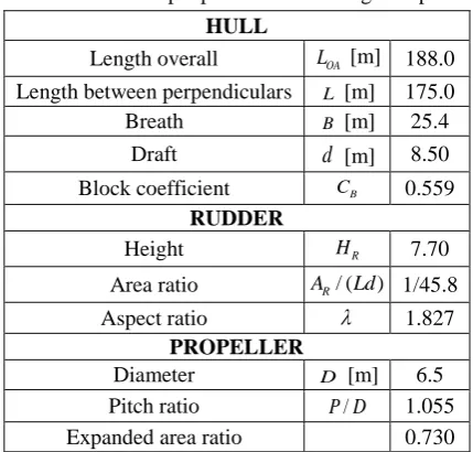
To build a mathematical model of ship maneuvering, a definition of a coordinate system and principal particulars of a ship
are first presented in Fig. 1 and Table 1, respectively. And then, a mathematical model of ship maneuvering and modeling of a
propeller and rudder are presented in the following two subsections.
Fig. 1 Coordinate system
where x and y are the actual positions of the ship in meters, and and
are the normalized positions of x y, by the length of the ship.Table 1 Principal particulars of a target ship
HULL
Length overall LOA [m] 188.0 Length between perpendiculars L [m] 175.0
Breath B [m] 25.4
Draft
d
[m] 8.50Block coefficient CB 0.559 RUDDER
Height HR 7.70
Area ratio AR/ (Ld) 1/45.8
Aspect ratio 1.827
PROPELLER
Diameter D [m] 6.5
Pitch ratio P D/ 1.055
2.1. Mathematical model for ship-maneuvering problem
In the ship-maneuvering problem, a planar motion includes only surge, sway and yaw motions, which are considered out
of six-degree-of-freedom motions. The basic equations of motion for ship maneuvering can be expressed as follows:
( ) surge
m uvr F (1)
( ) sway
m vur F (2)
z yaw
I r
M
(3)where m is the mass, and
u v r
, ,
are the velocities in the surge, sway, yaw directions, respectively.I
z is the moment ofinertia with respect to the z-axis, and Fsurge,Fsway,Fyaw are the surge and sway forces and yaw moment, respectively. The dot represents the time derivative. The right terms in Eqs. (1)-(3) can be dealt with using the established procedure from Newman
[24], and Eqs. (1)-(3) can be expressed as Eqs. (4)-(6).
(m m u x) (m m vr y) X (4)
(m m v y) (m m ur x) Y (5)
(
I
z
J r
z)
N
x Y
G (6)where mx,my,Jz are the added mass in the surge and sway directions and the added moment of inertia, respectively. X Y, are the hydrodynamic forces, and N is the hydrodynamic moment.
x
G is the distance from the midship to the center of gravity. The hydrodynamic forces and moment are generally expressed as Eqs. (7)-(9), which were proposed by theManeuvering Modeling Group (MMG).
H P R W T
XX X X X X (7)
H P R W T
YY Y Y Y Y (8)
H P R W T
NN N N N N (9)
where subscripts
H P R W T
, , , ,
refer to the hull, propeller, rudder, wind and tug, respectively. However, due to this paperfocuses on the application of recent developments in DL; the external forces such as the wind and tug are not considered.
A ship’s maneuvering displacements and velocities can be calculated numerically by integrating Eq. (10)-(12) using the
Runge–Kutta 4th-order method.
( )
( )
y
x X m m vr u m m (10) ( ) ( ) x y Y m m ur v m m (11) G z z
N x Y
r
I J
(12)
2.2 Modeling of propeller and rudder
Owing to the kinematics of the mechanical system of the rudder and engine, time delays between commands of operation
and the resultant mechanical response may occur. The equations from Shon [13] to consider this physical time-delay effect are
*
/ n
n n n T (13)
where n is the RPS, n is a derivative of RPS with respect to time, and *
n is the target RPS. Tn is a time-delaying constant for the RPS, and this variable is set to 15 s in this paper. Next, equations to consider the time-delay effect for a rudder are Eqs.
(14)-(15).
* *
max
( ) /TE; | | TE| |
(14)* *
max max
( )| |; | |> E| |
sign T
(15)where
* is the target rudder angle,E
T is the time-delaying constant for the rudder, and
max is the maximum angular velocity of the rudder. In this paper, TE is set to 2.5 s, and
max is set to 3.0°/s.3.
Artificial Neural Network and Important Factors in Training the Network
3.1. Artificial neural network
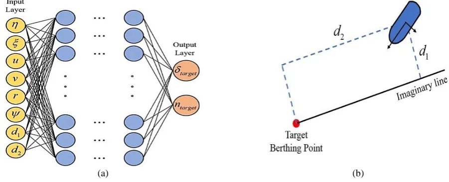
The basic architecture of the neural network used in this paper is illustrated in Fig. 2, is x/L, and
is y/L, in which,
x y are the relative positions of the ship from the target berthing point, and
L
is the LBP of the ship. u v r, , are the velocities of the ship in the surge, sway, and yaw directions, respectively, and is the heading angle of the ship. In the outputlayer,
target,ntarget are the target rudder angle and target RPS, respectively. This input layer configuration has been used in several papers such as those of Im and Hasegawa [1] and Ahmed and Hasegawa [5]. The number of hidden layers and the sizeof the neural network will be addressed in Section 3.5.
(a) (b)
Fig. 2 Basic architecture of neural network, and concept of imaginary line
The imaginary line shown in Fig. 2 is used as a guideline during berthing. It is known that as the imaginary line provides
the additional input variables of d1 and d2, which can improve the berthing performance by the neural network. The angle between the x-axis and the imaginary line is set to 20° in this paper.
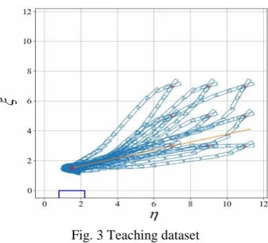
For the teaching data preparation, the patterns of the berthing trajectories, rudder angle, and RPS control from Nguyen
and Im [14] and Bae et al. [4] are referred. The teaching dataset used in this paper is shown in Fig. 3, where the red crosses are
Fig. 3 Teaching dataset
The end of the berthing operation is defined as a status meeting and the following three conditions according to Ahmed
and Hasegawa [15]. First, the aim is to berth at a distance of around the length of 1.5 times farer than where the ship is from the
berthing facility. Second, the relative heading angle to the berthing facility should be smaller than 30°. Third, the velocity of
the ship should be slower than 0.2 m/s.
The overall flowchart for the automatic ship berthing with a neural network is shown in Fig. 4, the left side of the dotted
line is the preparation step for the neural network model, and the right side is a processing loop with the trained neural network.
In this paper, building and training the neural networks are carried out with the open-source software library Tensorflow
developed by the Google Brain Team.
Fig. 4 Flowchart for ANN-based ship berthing system
3.2. Activation function and weight initialization
Choosing both an appropriate activation function and weight initialization method is quite important in building a neural
network. The training performance and training speed can be greatly affected by these two parameters.
For the activation function, many previous studies such as those of Im [3], Bae et al. [4], Ahmed and Hasegawa [5], and
Lee and Lee et al. [26] used the sigmoid function. However, it is known that the sigmoid function intrinsically has some
disadvantages in training neural networks. According to Nwankpa et al. [25], the drawbacks of the sigmoid function are sharp
damp gradients during backpropagation, gradient saturation, slow convergence, and nonzero-centered output. Thus, many
studies have been carried out to develop better activation functions to overcome the problems of the sigmoid function. The
activation functions that are popularly used these days are the tangent hyperbolic and Rectified Linear Unit (ReLu) functions
proposed by Nair and Hinton [7]. The tangent hyperbolic function solves the problem of the limitation in the gradient update
direction that exists in the sigmoid function, and results in a faster training speed. The ReLu function avoids the gradient
vanishing problem and lowers the complexity of the calculations as its derivative function is relatively simple. The equations
for the sigmoid, tangent hyperbolic, and ReLu functions are shown in Eqs. (16)-(18):
( ) 1/ 1 x
x x
x x
e e tanh(x)=
e e
(17)
( ) ; 0
( ) 0;
relu x x x relu x otherwise
(18)
For the weight initialization method, the normal distribution with a mean of zero and a standard deviation of 0.01 was
mostly used. Later, however, many studies showed that the weight initialization method can greatly affect the training
performance, and many other weight initialization methods have been proposed. Among the proposed methods, the two most
popular at present are the Xavier initialization (also called the Glorot initialization) by Glorot and Bengio [16] and the He
initialization by He et al. [17]. According to Glorot and Bengio [16], the Xavier initialization results in good training
performance with the sigmoid and tanh functions. According to He et al. [17], the He initialization is very compatible with the
ReLu function. The equations for the Xavier and He initialization methods are based on a normal distribution where a mean
value is set to zero and variance is set to Eq. (19) for the Xavier initialization and Eq. (20) for the He initialization.
2
Xavier 2 / nin nout
(19)
2
He
2 /
n
in
(20)where
n
in andn
out represent the numbers of the previous and next layer’s nodes.3.3. Optimizer
In previous studies, such as those of Im and Hasegawa[1], Im and Hasegawa [2], Im [3], Ahmed and Hasegawa [5], and
Im and Nguyen [6] adopted the Levenberg–Marquardt approach proposed by Levenberg [9]. However, according to Bazzi et al.
[10], who analyzed the training performance of several popular optimizers including Levenberg–Marquardt, the Root Mean
Square Propagation (RMSProp) method proposed by Tieleman and Hinton [11] is faster and computationally more efficient,
and requires fewer hyperparameters than Levenberg–Marquardt. Furthermore, Kingma and Ba [12] showed that the Adam
optimizer proposed by Kingma and Ba [12], which is a combination of RMSprop and Momentum proposed by Rumelhart et al.
[19], outperforms RMSprop. Therefore, Adam is adopted as an optimizer in this paper. The learning rate of the Adam is set to
1e-3, which results in a robust training performance in general. For the loss function to be minimized by Adam, the Mean
Square Error (MSE) is used.
3.4. Input data scaling
Table 2 List of input data-scaling methods
Scaling #1 0 to 1 Min-Max Scaling Scales inputs to range of 0 to 1
Scaling #2 -1 to 1 Min-Max Scaling Scales inputs to range of -1 to 1
Scaling #3 Standard Scaling Standardizes inputs by removing mean and scaling to unit variance
Because the input data of a ship berthing dataset for neural network contains variables of different units, the weights are
likely to be updated in an unstable way during training when input data scaling is not applied because of the different scales of
each input variable. However, among the previous studies on ANN-based automatic berthing, some did not employ a scaling
method for their input data, and some applied a scaling method on some input variables only. A few of the studies scaled the
input data to between 0 and 1. The commonly used input data-scaling methods are presented in Table 2 and Eqs. (21)-(23).
( min( )) / (max( ) min( ))
x x X X X (21)
( 2 min( )) / (max( ) min( ))
( ( )) / ( )
x x mean X std X (23)
where x is the sampled data,
x
is the scaled sampled data, andX
is a set of data.3.5. Number of hidden layers
The number of hidden layers has a close relationship with the neural network model’s system capacity. It is commonly
known that if a neural network model has a large number of hidden layers; it has a large capacity to understand the complexity
of a given training dataset and to have a complex system. However, simply using many hidden layers does not guarantee the
neural network’s good performance. Numbers of hidden layers of 5, 10, 20, 30, and 40 are considered and investigated in
Section 4. The hidden layer size is also an important factor in the neural network architecture, but in order to build a neural
network model for a complex system, the number of hidden layers is more influential. Generally, the hidden layer size is set to
2n. n is 5 for simple systems, 6 for a slightly complex systems, and 8–9 for complex systems. In this paper, the hidden layer size
is set to 26.
3.6. Overfitting prevention
Algorithm 1 Batch Normalization
Input: Values of x over a mini-batch: {x1 ... m};Parameters to be learned: ,
Output:
BN , ( )}i iy x
1 1 m i i x m
// mini-batch mean2 2 1 1 ( ) m i i x m
// mini-batch variance2
ˆ xi
x
// normalize
γ,
ˆ
γx BN ( )
i i i
y
x // scale and shiftOverfitting may occur when a neural network is trained with a given training dataset over many epochs because the
weights become too fit to the given dataset only. Then, the performance of the neural network fails with new input data. In an
automatic berthing using a neural network, if overfitting occurs, the neural network will show poor berthing performance when
a new initial position is given. The poor performance with the overfitting issue occurs more clearly when new input data is
extrapolated rather than interpolated by the neural network. In previous studies on ANN-based automatic berthing, no
regularization methods to prevent overfitting were considered. Some papers such as Bae et al. [4] showed that poor berthing
performance occurs owing to an extrapolated initial position. In order to deal with the poor performance caused by the
extrapolation, the BN is adopted. The advantages of the BN are as follows. It allows for a higher learning rate, reduces the
dependence of initial weights, and provides a regularization effect to prevent overfitting. The pseudocode of BN is shown in
Algorithm 1. Where is a small value of about 10-6 to prevent division by zero.
4.
Application of Recent Developments in Deep Learning to Automatic Berthing
In this section, the effects of activation functions, weight initialization methods, input data-scaling methods, numbers of
hidden layers, and the BN that were introduced in the previous section are investigated in terms of the neural network’s training
As to the activation functions and weight initialization methods, nine different neural network models with nine
combinations from three activation functions of the sigmoid, tangent hyperbolic (tanh), and ReLu; and three weight
initialization methods of the normal distribution, Xavier, and He are built. In order to show the training progress over epochs,
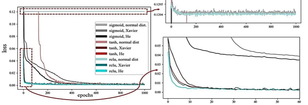
a loss function history graph is presented in Fig. 5. Details of the training models are listed in Table 3 for better reproducibility.
Fig. 5 Loss function histories with respect to activation and weight initialization methods
Table 3 Details of training models with respect to activation and weight initialization methods Hidden layer size Number of hidden layers Optimizer, learning rate Number of epochs Batch size Activation
function Weight initialization
Input data-scaling
method
26 10 Adam,
1e-3 1000 2
7 sigmoid,
tanh, ReLu
normal distribution, Xavier, He
-1 to 1 Min-Max Scaling
The number of hidden layers is set to 10 to make use of Deep Neural Networks (DNNs). The effect of the number of
hidden layers is investigated later in this section. The batch size is set to 27 because this is usually set to 2n, where n is generally
5 to the minimum and 10 to the maximum.
In Fig. 5, the models with weight initialization by normal distribution led to a slow training speed and poor convergence.
The models using the sigmoid function show a slow training speed as well. It is shown that the traditional activation function
and weight initialization method are inefficient in terms of training the DNN for automatic ship berthing. The best combination
of the activation function and weight initialization method is ReLu-He. He et al. [17] claimed that the ReLu function is very
compatible with He weight initialization.
For the input data-scaling methods, the effect of each input data-scaling method is analyzed with a loss function history.
The loss function history is shown in Fig. 6, and details of the training models with respect to the input data-scaling method are
listed in Table 4.
Table 4 Details of training models with respect to activation and weight initialization methods Hidden layer size Number of hidden layers Optimizer, learning rate Number of epochs Batch size Activation function Weight
initialization Input data-scaling method
26 10 Adam,
1e-3 1000 2
7 ReLu He
No Scaling, x y-Only Scaling, 0 to 1 Min-Max Scaling, -1 to 1 Min-Max Scaling,
Standard Scaling
Where the training model with No Scaling means that the input data of
x y u v r, , , , ,,d1,d2
, where x y, are the actual,
In Fig. 6, the significance of application of the input data-scaling method is clearly seen by its training speed and
convergence. Standard Scaling shows the fastest training speed and best convergence with the least oscillation, while No
Scaling resulted in poor training performance.
Fig. 6 Loss function histories with respect to input data-scaling methods
Next, the effect of the number of hidden layers is analyzed based on the loss function history and berthing performance
history with initial positions from the training dataset. The berthing performance history is obtained as in Algorithm 2.
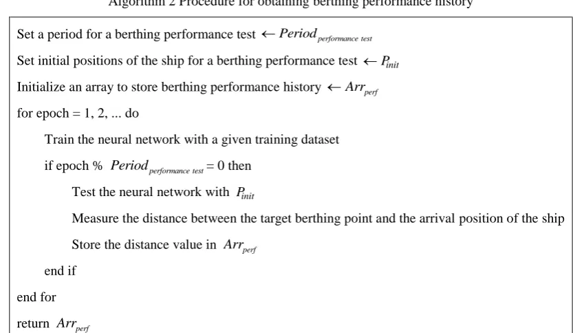
Algorithm 2 Procedure for obtaining berthing performance history
Set a period for a berthing performance test
Set initial positions of the ship for a berthing performance test Pinit
Initialize an array to store berthing performance history Arrperf for epoch = 1, 2, ... do
Train the neural network with a given training dataset
if epoch % Periodperformance test= 0 then Test the neural network with Pinit
Measure the distance between the target berthing point and the arrival position of the ship
Store the distance value in Arrperf
end if
end for
return Arrperf
The loss function history and berthing performance history with initial positions of the ship from the training dataset with
respect to the number of hidden layers are shown in Fig. 7. Details of the training models are listed in Table 5. In Fig. 7(a),
n_hidden_layer of 5 and 10 result in the most stable training, whereas the others show somewhat unstable training with fluctuations. In Fig. 7(b), the y-axis of the distance represents the distance gap between the target berthing point and arrival
position of the ship, as shown in Algorithm 2. Thus, when the distance is zero, this indicates the highest value and thus the
highest performance. The edges of the shaded areas in Fig. 7(b) represent the actual data. It is shown that the training model
with the n_hidden_layer of 10 shows the highest performance, and an unnecessarily complex neural network model with many
hidden layers decreases the performance.
Table 5 Details of training models with respect to number of hidden layers Hidden
layer size
Number of hidden layers
Optimizer, learning rate
Number of
epochs Batch size
Activation function
Weight initialization
Input data-scaling method
26 5, 10, 20, 30, 40 Adam, 1.0e-3 1000 27 ReLu He Standard Scaling
performance test Period
(a) Loss function histories
(b) Berthing performance histories with initial positions from training dataset
Fig. 7 Loss function and berthing performance histories with respect to number of hidden layers
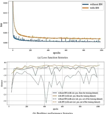
Finally, to verify the model’s universal berthing performance, the effect of using the BN to prevent overfitting and to
improve the neural network’s performance is analyzed by the loss function history and berthing performance history with
initial positions from the training dataset and a set of new initial positions that are not included in the training dataset. The set
of new initial positions is shown in Fig. 8, where the red crosses are the initial positions in the teaching data and the blue ships
represent the new initial positions.
Fig. 8 Set of new initial positions for berthing performance history to verify universal berthing performance
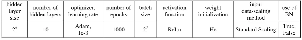
Table 6 Details of training models when BN is used hidden
layer size
number of hidden layers
optimizer, learning rate
number of epochs
batch size
activation function
weight initialization
input data-scaling
method
use of BN
26 10 Adam,
1e-3 1000 2
7 ReLu He Standard Scaling True,
False
The loss function and berthing performance histories, and details of the training models with respect to the use of the BN,
training process. The performances in Fig. 9(b) show that the model with BN outperforms the model without BN not only for the
initial positions from the training dataset but also for the new initial positions that are not included in the training dataset.
(a) Loss function histories
(b) Berthing performance histories
Fig. 9 Loss function and berthing performance histories when BN is used
Algorithm 3 Trained model selection algorithm for neural networks for automatic ship berthing
Initialize an array to store harmonic mean values Arrhm
Set the berthing performance history data with the initial positions from the training dataset X
Set the berthing performance history data with the new initial positions out of the training dataset Y
for each xX and yY then Concatenate
X
andY
XY
min( ) / max(
) min( )
x x XY XY XY // 0 to 1 Min-max Scaling
min( ) / max(
) min( )
y y XY XY XY
2
/
hm x y xy // harmonic mean Store
hm
in Arrhmend for
Index of the best model is arg max(Arrhm)
Although the trained model with the BN shows good and stable performance over epochs, it is ideal to select the
best-trained model of them all. In order to select the best-trained model, a trained model selection algorithm for neural network
models for automatic berthing using the harmonic mean is proposed. The trained model selection algorithm is shown in
Algorithm 3.
We adopted the harmonic mean to penalize cases where the gap between the berthing performances with the initial
positions from and out of the training dataset is high, meaning that the model is overfit to the given training dataset and has a
poor universal berthing performance. It has been shown that the use of the recent activation functions, weight initialization
method, and input data-scaling methods resulted in faster training speeds and better convergence of the loss function. In
addition, the BN improved the actual berthing performance for universal use and stabilized the training process. With the
trained model selection algorithm, the two best-trained models were selected for the final simulation in Section 5. One is from
the trained models with the BN, and the other is from the trained models without the BN. The significance of the BN
application is shown and discussed in the next section.
5.
Simulation and Results Discussion
In this section, the berthing trajectories by two different trained models with and without the BN are presented to show
how the BN improves the neural network for ship berthing and solves the extrapolation problem. First, berthing trajectories
with the initial positions from the training dataset are presented. And then, the berthing trajectories with interpolated and
extrapolated initial positions are presented next, respectively. In the berthing simulations in this section, the initial u is set to
1.5, and the initial n is set to 0.5 for all cases.
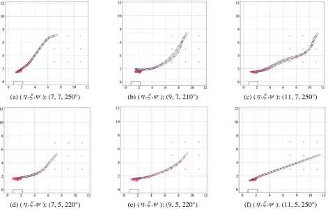
To validate if the two trained neural network models perform efficiently when initial positions from a training dataset are
given, berthing trajectories with initial positions from a training dataset are presented in Fig. 10. As expected from the berthing
performance history in Fig. 9(b), similar berthing performance and trajectories are shown with the initial positions from the
training dataset as shown in Fig. 10(a)-(i), meaning that both trained models are trained well for the given training dataset.
(a) ( , , ): (7, 7, 250°) (b) ( , , ): (9, 7, 210°) (c) ( , , ): (11, 7, 250°)
(d) ( , , ): (7, 5, 220°) (e) ( , , ): (9, 5, 220°) (f) ( , , ): (11, 5, 250°)
To validate if the two trained neural network models perform efficiently when interpolated initial positions are given,
berthing trajectories with the interpolated initial positions are presented in Fig. 11. It can be observed that when the interpolated
initial positions are given, both trained models showed successful berthing performances with similar berthing trajectories as
shown in Fig. 11(a)-(f)
In the following simulations, the trained models are given three types of extrapolated initial positions. The types of
extrapolated initial positions differ by the magnitude of extrapolation.
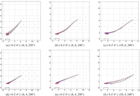
Berthing trajectories with the first type of extrapolated initial position are shown in Fig. 12. It can be observed that although
the trained model without the BN shows good berthing performance in a few cases such as Fig. 12(a)-(b), it also shows poor
performance as shown in Fig. 12(c)-(d), while the model with the BN performs successfully in all the cases. In addition, it can be
seen that the two trained models control quite differently to reach the target berthing point, as seen in Fig. 12(e)-(f). (g) ( , , ): (7, 3, 270°) (h) ( , , ): (9, 3, 270°) (i) ( , , ): (11, 3, 270°)
Fig. 10 Berthing trajectories with initial positions from training dataset (red: with BN, blue: without BN) (continued)
(a) ( , , ): (6, 6, 220°) (b) ( , , ): (8, 6, 240°) (c) ( , , ): (10, 6, 240°)
(d) ( , , ): (6, 4, 240°) (e) ( , , ): (8, 4, 250°) (f) ( , , ): (10, 4, 240°)
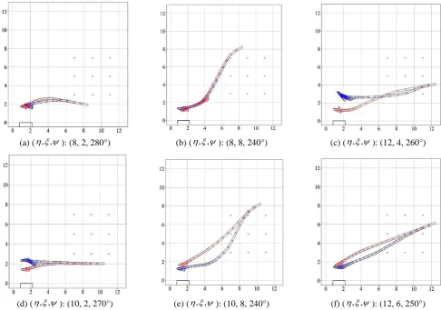
(a) ( , , ): (8, 2, 280°) (b) ( , , ): (8, 8, 240°) (c) ( , , ): (12, 4, 260°)
(d) ( , , ): (10, 2, 270°) (e) ( , , ): (10, 8, 240°) (f) ( , , ): (12, 6, 250°)
Fig. 12 Berthing trajectories with extrapolated initial positions, Type 1 (red: with BN, blue: without BN)
(a) ( , , ): (14, 2, 280°) (b) ( , , ): (14, 4, 260°) (c) ( , , ): (8, 10, 210°)
(d) ( , , ): (10, 10, 230°) (e) ( , , ): (12, 10, 250°) (f) ( , , ): (14, 6, 250°)
Next, berthing trajectories with the second type of extrapolated initial position are shown in Fig. 13. As the more
extrapolated initial positions are given in the cases in Fig. 13, the trained model without the BN suffers from the extrapolation
issue even more as shown in Fig. 13(a)-(e). The only case where the trained model without the BN performs well is when it
berths in a straight line as shown in Fig. 13(f).
Finally, berthing trajectories with the third type of extrapolated initial position are shown in Fig. 14, in which the
extrapolation of initial positions is the greatest in order to clearly see the effect of the BN. In Fig. 14. The model without the BN
performs poorly overall owing to the extrapolation problem. The effectiveness of application of the BN is clear, as the BN
improves the neural network model for more general use.
6.
Conclusion
We showed that with the application of recent activation functions, weight initialization methods, input data-scaling
methods, and a higher number of hidden layers, faster training speed and better training convergence can be achieved. In order
to observe the progress of the berthing performance over epochs and select the best-trained model, the algorithm for obtaining
the berthing performance history and the model selection algorithm were proposed as Algorithms 2 and 3, respectively. Last,
the use of the BN can stabilize the training process and solve the extrapolation problem by preventing overfitting. A neural
network model with the BN was able to perform successfully, not only with interpolated and slightly extrapolated initial
positions but also with greatly extrapolated initial positions. This makes the neural network models more universal for
automatic berthing.
Acknowledgement
This material is based upon work supported by the Ministry of Trade, Industry & Energy (MOTIE, Korea) under
Industrial Technology Innovation Program. No. 10063405, “Development of hull form of year-round floating-type offshore
structure based on the Arctic Ocean in ARC7 condition with dynamic positioning and mooring system.”
(a) ( , , ): (18, 4, 270°) (b) ( , , ): (14, 6, 260°) (c) ( , , ): (18, 6, 230°)
(d) ( , , ): (8, 14, 180°) (e) ( , , ): (10, 14, 190°) (f) ( , , ): (14, 14, 210°)
Conflicts of Interest
The authors declare no conflict of interest.
References
[1] N. K. Im and K. Hasegawa, “Automatic ship berthing using parallel neural controller,” Proc. International Federation of Automatic Control (IFAC), vol. 34, no. 7, pp. 51-57, 2001.
[2] N. K. Im and K. Hasegawa, “Motion identification using neural networks and its application to automatic ship berthing under wind,” Journal of Ship and Ocean Technology, vol. 6, no. 1, pp. 16-26, 2002.
[3] N. K. Im, “All direction approach automatic ship berthing controller using ANN (artificial neural networks),” Journal of Institute of Control, Robotics and Systems, vol. 13, no. 4, pp. 304-308, 2007.
[4] C. H. Bae, S. K. Lee, S. E. Lee, and J. H. Kim, “A study of the automatic berthing system of a ship using artificial neural network,” Journal of Korean Navigation and Port Research, vol. 32, no. 8, pp. 589-596, 2008.
[5] Y. A. Ahmed and K. Hasegawa, “Automatic ship berthing using artificial neural network trained by consistent teaching data using nonlinear programming method,” Engineering Applications of Artificial Intelligence, vol. 26, no. 10, pp. 2287-2304, 2013.
[6] N. K. Im and V. S. Nguyen, “Artificial neural network controller for automatic ship berthing using head-up coordinate system,” International Journal of Naval Architecture and Ocean Engineering, vol. 10, no. 3, pp. 235-249, 2018. [7] V. Nair and G. E. Hinton, “Rectified linear units improve restricted Boltzmann machines,” Proc. 27th International
Conference on Machine Learning (ICML-10), 2010.
[8] A. L. Maas, A. Y. Hannun, and A. Y. Ng, “Rectifier nonlinearities improve neural network acoustic models,” Proc. International Conference on Machine Learning, vol. 30, no. 1, 2013.
[9] K. Levenberg, “A method for the solution of certain non-linear problems in least squares,” Quarterly of Applied Mathematics, vol. 2, no. 2, pp. 164-168, 1944.
[10] T. Bazzi, R. Ismail, and M. Zohdy, “Comparative performance of several recent supervised learning algorithms,” International Journal of Computer and Information Technology, vol. 7, 2018.
[11] T. Tieleman and G. Hinton, Lecture 6.5-rmsprop: Divide the gradient by a running average of its recent magnitude, COURSERA: Neural Networks for Machine Learning, 2012.
[12] D. P. Kingma and J. Ba, “Adam: a method for stochastic optimization,” arXiv preprint arXiv:1412.6980, 2014.
[13] K. H. Shon, “Hydrodynamic forces and maneuvering characteristics of ships at low advance speed,” Journal of the Society of Naval Architects of Korea, vol. 29, no. 3, pp. 90-101, 1992.
[14] V. S. Nguyen, V. C. Do, and N. K. Im, “Development of automatic ship berthing system using artificial neural network and distance measurement system,” International Journal of Fuzzy Logic and Intelligent Systems, vol. 18, no. 1, pp. 41-49, 2018. [15] Y. A. Ahmed and K. Hasegawa, “Automatic ship berthing using artificial neural network based on virtual window concept
in wind condition,” Proc. International Federation of Automatic Control (IFAC), vol. 45, no. 24, pp. 286-291, 2012. [16] X. Glorot and Y. Bengio, “Understanding the difficulty of training deep feedforward neural network,” Proc. International
Conference on Artificial Intelligence and Statistics, vol. 9, pp. 246-266, 2010.
[17] K. He, X. Zhang, S. Ren, and J. Sun, “Delving deep into rectifiers: surpassing human-level performance on Imagenet classification,” Proc. IEEE International Conference on Computer Vision, pp. 1026-1034, 2015.
[18] H. Robbins and S. Monro, “A stochastic approximation method,” The Annals of Mathematical Stastics, pp. 400-407, 1951. [19] D. E. Rumelhart, G. E. Hinton, and R. J. Williams, “Learning representations by back-propagating errors,” Nature, vol. 323,
no. 6088, pp. 533-536, 1986.
[20] J. Duchi, E. Hazan, and Y. Singer, “Adaptive subgradient methods for online learning and stochastic optimization,” Journal of Machine Learning Research, pp. 2121-2159, July 2011.
[21] C. M. Bishop, Neural networks for pattern recognition. Oxford: Clarendon Press, New York, 1996.
[22] N. Srivastava, G. Hinton, A. Krizhevsky, I. Sutskever, and D. Salakhutdinov, “Dropout: A simple way to prevent neural networks from overfitting,” Journal of Machine Learning Research, vol. 15, no.1, pp. 1929-1958, 2014.
[23] S. Loffe and C. Szegedy, “Batch normalization: Accelerating deep network training by reducing internal covariate shift,” arXiv preprint arXiv:1502.03167, 2015.
[24] J. N. Newman, Marine hydrodynamics. Cambridge, MA: MIT Press, 1980.
[25] C. Nwankpa, W. Ijomah, A. Gachagan, and S. Marshall, “Activation functions: comparison of trends in practice and research for deep learning,” arXiv preprint arXiv:1811.03378, 2018.
[26] S. K. Lee, G. W. Lee, S. J. Lee, and S. R. Jeong, “A study on the automatic berthing control of a ship by artificial neural network,” Journal of Korean Navigation and Port Research, vol. 32, no. 4, pp. 21-28, 1997.
Copyright© by the authors. Licensee TAETI, Taiwan. This article is an open access article distributed under the terms and conditions of the Creative Commons Attribution (CC BY-NC) license