The Locally Weighted Bag of Words Framework for Document Representation

The Locally Weighted Bag of Words Framework for Document

Representation

Guy Lebanon [email protected]

Yi Mao [email protected]

Joshua Dillon [email protected]

Department of Statistics and

School of Electrical and Computer Engineering Purdue University - West Lafayette, IN, USA

Editor: Andrew McCallum

Abstract

The popular bag of words assumption represents a document as a histogram of word occurrences. While computationally efficient, such a representation is unable to maintain any sequential infor-mation. We present an effective sequential document representation that goes beyond the bag of words representation and its n-gram extensions. This representation uses local smoothing to embed documents as smooth curves in the multinomial simplex thereby preserving valuable sequential in-formation. In contrast to bag of words or n-grams, the new representation is able to robustly capture medium and long range sequential trends in the document. We discuss the representation and its geometric properties and demonstrate its applicability for various text processing tasks.

Keywords: text processing, local smoothing

1. Introduction

Modeling text documents is an essential component in a wide variety of text processing applica-tions, including the classification, segmentation, visualization and retrieval of text. A crucial part of the modeling process is choosing an appropriate representation for documents. In this paper we demonstrate a new representation that considers documents as smooth curves in the multinomial simplex. The new representation goes beyond standard alternatives such as the bag of words and n-grams and captures sequential content at a certain resolution determined by a given local smoothing operator.

We consider documents as finite sequences of words

y=_hy1, . . . ,yNi yi∈V (1)

where V represents finite vocabulary which for simplicity is assumed to be a set of integers V = {1, . . . ,_|V_|}=_{1, . . . ,V_}. The slight abuse of notation of using V once as a set and once as an integer will not cause confusion later on and serves to simplify the notation. Due to the categorical or nominal nature of V , a document should be considered as a categorical valued time series. In typical cases, we have 1<NV which precludes using standard tools from categorical time series

in a Euclidean spaceRVn which is a convenient representation, albeit high dimensional, for many machine learning and statistical models. The specific case of n=1, also called bag of words or bow representation, is perhaps the most frequent document representation due to its relative robustness in sparse situations.

Formally, the n-gram approach represents a document y=_hy1, . . . ,yNi,yi∈V as x∈RV n

, defined by

x₍j1,...,jn)= 1

N₋n+1

N−n+1

∑

δyi,j1δyi+1,j2···δyi+n−1,jn, (2)

whereδa,b=1 if a=b and 0 otherwise. In the case of 1-gram or bag of words the above represen-tation reduces to

xj= 1

N

N

∑

δyi,j

which is simply the relative frequencies of different vocabulary words in the document.

A slightly more general outlook is to consider smoothed versions of (2) in order to avoid the oth-erwise overwhelmingly sparse frequency vector (since NV , only a small subset of the vocabulary

appears in any typical document). For example, a smoothed 1-gram representation is

xj= 1

Z

N

∑

(δyi,j+c), c≥0 (3)

where Z is a constant that ensures normalization∑xj=1. The smoothed representation (3) has a Bayesian interpretation as a the maximum posterior estimate for a multinomial model with Dirichlet prior and setting c=0 in (3) reduces it to the standard word histogram or 1-gram. Recent com-parative studies of various n-gram smoothing methods in the contexts of language modeling and information retrieval may be found in Chen and Rosenfeld (2000) and Zhai and Lafferty (2001).

Conceptually, we may consider the n-gram representation for n=N in which case the full

original sequential information is maintained. In practice, however, n is typically chosen to be much smaller than N, often taking the values 1, 2, or 3. In these cases, frequently occurring word patterns are kept allowing some limited amount of word-sense disambiguation. On the other hand, almost all of the sequential content, including medium and long range sequential trends and position information is lost.

The paper’s main contribution is a new sequential representation called locally weighted bag of words or lowbow. This representation, first introduced in Lebanon (2005), generalizes bag of words by considering the collection of local word histograms throughout the document. In contrast to

n-grams, which keep track of frequently occurring patterns independent of their positions, lowbow

keeps track of changes in the word histogram as it sweeps through the document from beginning to end. The collection of word histograms is equivalent to a smooth curve which facilitates the differential analysis of the document’s sequential content. The use of bag of words rather than n-grams with n>1 is made here for simplicity purpose only. The entire lowbow framework may be generalized to define locally weighted n-grams in a straightforward manner.

by related work and discussion. Since our presentation makes frequent use of the geometry of the multinomial simplex, which is not common knowledge in the machine learning community, we provide a brief summary of it in Appendix A.

2. Locally Weighted Bag of Words

As mentioned previously, the original word sequence (1) is categorical, high dimensional and sparse. The smoothing method employed by the bag of words representation (3) is categorical in essence rather than temporal since no time information is preserved. In contrast to (3) or its variants, tempo-ral smoothing such as the one used in local regression or kernel density estimation (e.g., Wand and Jones, 1995) is performed across a continuous temporal or spatial dimension. Temporal smoothing has far greater potential than categorical smoothing since a word can be smoothed out to varying degrees depending on the temporal difference between the two document positions. The main idea behind the locally weighted bag of words framework is to use a local smoothing kernel to smooth the original word sequence temporally. In other words, we borrow the presence of a word at a cer-tain location in the document to a neighboring location but discount its contribution depending on the temporal distance between the two locations.

Since temporal smoothing of words results in several words occupying one location we need to consider the following broader definition of a document.

Definition 1 A document x of length N is a function x :_{1, . . . ,N_{} ×}V _→[0,1]such that

∑

x(i,j) =1 _∀i_{∈ {}1, . . . ,N_}.

The set of documents (of all lengths) is denoted byX_.

For a document x_∈X_{the value x(i,j)represent the weight of the word j∈V at location i. Since}

the weights sum to one at any location we can consider Definition 1 as providing a local word histogram or distribution associated with each document position. The standard way to represent a word sequence as a document inX_{is to have each location host the appropriate single word with}

constant weight, which corresponds to theδcrepresentation defined below with c=0.

Definition 2 The standard representationδc(y)∈X, where c≥0, of a word sequence y=hy1, . . . ,yNi

is

δc(y)(i,j) =

( _c

1+c|V| yi6= j

1+c

1+c|V| yi= j

. (4)

Equation (4) is consistent with Definition 1 since∑j∈Vδc(y)(i,j) =₁1+_+cc|_|V_V|_| =1. The parameter c in the above definition injects categorical smoothing as in (3) to avoid zero counts in theδc represen-tation.

The standard representationδcassumes that each word in the sequence y=hy1, . . . ,yNioccupies a single temporal location 1, . . . ,N. In general, however, Definition 1 lets several words occupy the

Definition 1 is problematic since according to it, two documents of different lengths are consid-ered as fundamentally different objects. It is not clear, for example, how to compare two documents

x1:{1, . . . ,N1} ×V →[0,1], x2:{1, . . . ,N2} ×V →[0,1]of varying lengths N16=N2. To allow a

unified treatment and comparison of documents of arbitrary lengths we map the set{1, . . . ,N}to a continuous canonical interval, which we arbitrarily choose to be[0,1].

Definition 3 A length-normalized document x is a function x :[0,1]_×V_→[0,1]such that

∑

x(t,j) =1, _∀t_∈[0,1].

The set of length-normalized documents is denotedX0_.

A simple way of converting a document x_∈X_{to a length-normalized document x}0_∈X0_{is expressed}

by the length-normalization function defined below.

Definition 4 The length-normalization of a document x_∈X_{of length N is the mapping}

ϕ:X_→X0 ϕ_{(x)(t,j) =x(dtNe,j)}

where_dr_eis the smallest integer greater than or equal to r.

The length-normalization process abstracts away from the actual document length and focuses on the sequential variations within the document relative to its length. In other words, we treat two documents with similar sequential contents but different lengths in a similar fashion. For example the two documents_hy1,y2, . . . ,yNi andhy1,y1,y2,y2, . . . ,yN,yNior the more realistic example of a news story and its summary would be mapped to the same length-normalized representation. The assumption that the actual length does not matter and sequential trends should be considered relative to the total length may not hold in some cases. We comment on this assumption further and on how to relax it in Section 7.

We formally define bag of words as the integral of length-normalized documents with respect to time. As we show later, this definition is equivalent to the popular definition of bag of words expressed in Equation (3).

Definition 5 The bag of words or bow representation of a document y isρ(ϕ(δc(y)))defined by

ρ:X0_{→PV−1 where [}ρ_(x)]j=

Z 1

0

x(t,j)dt, (5)

and[_·]jdenotes the j-th component of a vector.

Above,PV−1stands for the multinomial simplex

PV₋1= (

θ∈RV :_∀iθi≥0, V

∑

θj=1

)

which is the subset ofRV _{representing the set of all distributions on V events. The subscript V−1 is} used inPV−1rather than V in order to reflect its intrinsic dimensionality. The simplex and its Fisher

0 0.2 0.4 0.6 0.8 1 0 0.2 0.4 0.6 0.8 1

Figure 1: Beta (left) and bounded Gaussian (right) smoothing kernels for µ=0.2,0.3,0.4,0.5.

the necessary background and further details may be found in Kass and Voss (1997), Amari and Nagaoka (2000) and Lebanon (2005). Note that the functionρin Definition 5 is well defined since

∑

[ρ(x)]j=

∑

Z 1

0

x(t,j)dt=

Z 1

0 _j

∑

x(t,j)dt=

Z 1

0

1 dt=1 =_⇒ ρ(x)_∈PV−1.

A local alternative to the bag of words is obtained by integrating a length-normalized document with respect to a non-uniform measure on[0,1]. In particular, integrating with respect to a measure that is concentrated around a particular location µ_∈[0,1]provides a smoothed characterization of the local word histogram. In accordance with the statistical literature of non-parametric smoothing we refer to such a measure as a smoothing kernel. Formally, we define it as a function Kµ,σ:[0,1]→

Rparameterized by a location parameter µ_∈[0,1]and a scale parameterσ_∈(0,∞). The parameter

µ represents the (length-normalized) document location at which the measure is concentrated andσ

represents its spread or amount of smoothing. We further assume that Kµ,σ is smooth in t,µ and is normalized, that is,R1

0Kµ,σ(t)dt=1.

One example of a smoothing kernel on [0,1] is the Gaussian pdf restricted to [0,1] and re-normalized

Kµ,σ(x) =

( _{N(x ;µ,}σ₎

Φ((1−µ)/σ)−Φ(−µ/σ) x∈[0,1]

0 x_6∈[0,1] (6)

where N(x ; µ,σ) is the Gaussian pdf with mean µ and varianceσ2 andΦ is the cdf of N(x ; 0,1). Another example is the beta distribution pdf

Kµ,σ(x) =Beta

x ; βµ

σ,β

1₋µ

σ

(7)

Definition 6 The locally weighted bag of words or lowbow representation of the word sequence y isγ(y) =_{γµ(y): µ∈[0,1]}whereγµ(y)∈PV₋1is the local word histogram at µ defined by

[γµ(y)]j=

Z 1

0 ϕ

(δc(y))(t,j)Kµ,σ(t)dt. (8)

Equation (8) indeed associates a document location with a local histogram or a point in the simplex

PV₋1since

∑

[γµ(y)]j=

∑

Z 1

0

ϕ(δc(y))(t,j)Kµ,σ(t)dt=

Z 1

0

Kµ,σ(t)

∑

ϕ(δc(y))(t,j)dt

=

Z 1

0

Kµ,σ(t)·1 dt=1.

Geometrically, the lowbow representation of documents is equivalent to parameterized curves in the simplex. The following theorem establishes the continuity and smoothness of these curves which enables the use of differential geometry in the analysis of the lowbow representation and its properties.

Theorem 1 The lowbow representation is a continuous and differentiable parameterized curve in the simplex, in both the Euclidean and the Fisher geometry.

Proof We prove below only the continuity of the lowbow representation. The proof of

differentia-bility proceeds along similar lines. Fixing y, the mapping µ7→γµ(y) maps[0,1]into the simplex

PV₋1. Since Kµ,σ(t)is continuous on a compact region(µ,t)∈[0,1]2, it is also uniformly continuous and we have

lim

ε→0|[γµ(y)]j−[γµ+ε(y)]j|=εlim→0

Z 1

0 ϕ

(δc(y))(t,j)Kµ,σ(t)−ϕ(δc(y))(t,j)Kµ+ε,σ(t)dt

≤lim

ε→0

Z 1

0

ϕ(δc(y))(t,j)|Kµ,σ(t)−Kµ+ε,σ(t)|dt

≤lim

ε→0_t∈sup_[0,1]|Kµ,σ(t)−Kµ+ε,σ(t)|

Z 1

0 ϕ(δc(y))(t,j)dt =lim

ε→0_t∈sup_[0,1]|Kµ,σ(t)−Kµ+ε,σ(t)|=0.

As a result,

lim

ε→0kγµ(y)−γµ+ε(y)k2=

r

∑

|[γµ(y)]j−[γµ+ε(y)]j|2→0

proving the continuity ofγµ(y) in the Euclidean geometry. Continuity in the Fisher geometry fol-lows since it shares the same topology as the Euclidean geometry.

It is important to note that the parameterized curve that corresponds to the lowbow representa-tion consists of two parts: the geometric figure_{γµ(y): µ∈[0,1]} ⊂PV−1and the parameterization

it is easy to ignore the parameterization function when dealing with parameterized curves, one must be aware that different lowbow representations may share similar geometric figures but possess dif-ferent parameterization speeds. Thus it is important to keep track of the parameterization speed as well as the geometric figure.

The geometric properties of the curve depend on the word sequence, the kernel shape and the kernel scale parameter. The kernel scale parameter is especially important as it determines the amount of temporal smoothing employed. As the following theorem shows, ifσ_→∞the lowbow curve degenerates into a single point corresponding to the bow representation. As a consequence we view the popular bag of words representation (3) as a special case of the lowbow representation.

Theorem 2 Let Kµ,σ be a smoothing kernel such that when σ→∞, Kµ,σ(x) is constant in µ,x.

Then forσ_→∞, the lowbow curveγ(y) degenerates into a single point corresponding to the bow representation of (3).

Proof Since the kernel is both constant and normalized over [0,1], we have Kµ,σ(t) =1 for all

µ,t_∈[0,1]. For all µ_∈[0,1],

[γµ(y)]j=

Z 1

0 ϕ

(δc(y))(t,j)Kµ,σ(t)dt=

Z 1

0 ϕ

(δc(y))(t,j)dt

=

N

∑

1

N

δyi,j 1+c

1+c_|V_|+ (1−δyi,j)

c

1+c_|V_|

∝

∑

δyi,j(1+c) + (1−δyi,j)c∝ N

∑

(δyi,j+c).

Intuitively, small σwill result in a simplicial curve that quickly moves between the different corners of the simplex as the words y1,y2, . . . ,yN are encountered. The extreme case of σ→0 represents a discontinuous curve equivalent to the original word sequence representation (1). It is unlikely that either of the extreme casesσ_→∞orσ_→0 will be an optimal choice from a mod-eling perspective. By varyingσbetween 0 and∞, the lowbow representation interpolates between these two extreme cases and captures sequential detail at different resolutions. Selecting an appro-priate scale 0<σ<∞we obtain a sequential resolution that captures sequential trends at a certain resolution while smoothing away finer temporal details.

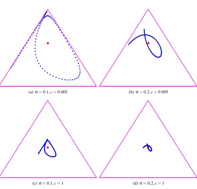
Figures 2-3 illustrate the curve resulting from the lowbow representation and its dependency on the kernel scale parameter and the smoothing coefficient. Notice how the curve shrinks asσ increases until it reaches the single point that is the bow model. Increasing c, on the other hand, pushes the geometric figure towards the center of the simplex.

0 0.1 0.2 0.3 0.4 0.5 0.6 0.7 0.8 0.9 1 0

0.1 0.2 0.3 0.4 0.5 0.6 0.7 0.8 0.9 1

(a)σ=0.1,c=0.005

0 0.1 0.2 0.3 0.4 0.5 0.6 0.7 0.8 0.9 1

0 0.1 0.2 0.3 0.4 0.5 0.6 0.7 0.8 0.9 1

(b) σ=0.2,c=0.005

0 0.1 0.2 0.3 0.4 0.5 0.6 0.7 0.8 0.9 1

0 0.1 0.2 0.3 0.4 0.5 0.6 0.7 0.8 0.9 1

(c)σ=0.1,c=1

0 0.1 0.2 0.3 0.4 0.5 0.6 0.7 0.8 0.9 1 0

0.1 0.2 0.3 0.4 0.5 0.6 0.7 0.8 0.9 1

(d) σ=0.2,c=1

Figure 2: The curve in P1 resulting from the lowbow representation of the word sequence h1 1

(a)σ=0.1,c=0.005 (b)σ=0.2,c=0.005

(c)σ=0.1,c=1 (d)σ=0.2,c=1

Figure 3: The curve inP2resulting from the lowbow representation of the word sequenceh1 3 3

3 2 2 1 3 3_i. In this caseP2 is visualized as a triangle inR2 (see Figure 15 for

visu-alizingP2). The figures illustrate the differences as the scale parameter of the Gaussian

kernelσincreases from 0.1 to 0.2 (left vs. right column) and the smoothing coefficient

c varies from 0.005 to 1 (first vs. second row). Increasing the kernel scale causes some local features to vanish, for example the tail in the bottom left corner ofP2. In addition,

Definition 7 Let Kµ,σ(t) be a kernel that is Lipschitz continuous1 in µ with a Lipschitz constant

CK(t). The kernel’s complexity is defined as

O

Z 1

0

CK(t)dt.

The theorem below proves that the lowbow curve is Lipschitz continuous with a Lipschitz constant

O

Theorem 3 The lowbow curveγ(y)satisfies

kγµ(y)−γτ(y)k2 ≤ |µ−τ|

O

|[γµ(y)]j−[γτ(y)]j| ≤

Z 1

0 ϕ

(δc(y))(t,j)|Kµ,σ(t)−Kτ,σ(t)|dt

≤

Z 1

0 |

Kµ,σ(t)−Kτ,σ(t)|dt

≤|µ₋τ_|

Z 1

0

CK(t)dt

and so_kγµ(y)−γτ(y)k2= q

∑j∈V|[γµ(y)]j−[γτ(y)]j|2≤ |µ−τ|

O

3. Modeling of Simplicial Curves

Modeling functional data such as lowbow curves is known in the statistics literature as functional data analysis (e.g., Ramsay and Dalzell, 1991; Ramsay and Silverman, 2005). Previous work in this area focused on low dimensional functional data such as one dimensional or two dimensional curves. In this section we discuss some issues concerning generative and conditional modeling of lowbow curves. Additional information regarding the practical use of lowbow curves in a number of text processing tasks may be found in Section 5.

Geometrically, a lowbow curve is a point in an infinite product of simplices P[V0₋,11] that is

nat-urally equipped with the product topology and geometry of the individual simplices. In practice, maintaining a continuous representation is often difficult and unnecessary. Sampling the path at rep-resentative points µ1, . . . ,µl∈[0,1]provides a finite dimensional lowbow representation equivalent to a point in the product spacePlV−1. Thus, even though we proceed below to consider continuous

curves and infinite dimensional spacesP[V0−,11], in practice we will typically discretize the curves and

replace integrals with appropriate summations.

Given a Riemannian metric g on the simplex, its product form

g0_θ(u,v) =

Z 1

0

g_θ(t)(u(t),v(t))dt

defines a corresponding metric on lowbow curves. As a result, geometric structures compatible with the base metric g, such as distance or curvature, give rise to analogous product versions. For

example, the distance between lowbow representations of two word sequencesγ(y),γ(z)_∈P[m0,1] is the average distance between the corresponding time coordinates

d(γ(y),γ(z)) =

Z 1

0

d(γµ(y),γµ(z))dµ (9)

where d(γµ(y),γµ(z)) depends on the simplex geometry under consideration, e.g. Equation (21) in the case of the Fisher geometry or d(γµ(y),γµ(z)) =kγµ(y)−γµ(z)k2 in the case of Euclidean

geometry.

Using the integrated distance formula (9) we can easily adapt distance-based algorithms to the lowbow representation. For example, k-nearest neighbor classifiers are adapted by replacing stan-dard distances such as the Euclidean distance or cosine similarity with the integrated distance (9) or its discretized version.

In contrast to the base distance onPV−1which is used in the bow representation, the integrated

distance (9) captures local differences in text sequences. For example, it compares the beginning of document y with the beginning of document z, the middle with the middle, and the end with the end. While it may be argued that the above is not expected to always accurately model differences between documents, it does hold in some cases. For example, news articles have a natural semantic progression starting with a brief summary at the beginning and delving into more detail later on, often in a chronological manner. Similarly, other documents such as web pages and emails share a similar sequential structure. Section 5.3 provides some experimental support for this line of thought and also describes some alternatives.

In a similar way, we can also apply kernel-based algorithms such as SVM to documents using the lowbow representation by considering a kernel overPV[0−,11]. For example, the product geometry

may be used to define a product diffusion process whose kernel can conveniently capture local relationships between documents. Assuming a base Fisher geometry we obtain the approximated diffusion kernel

Kt(γ(y),γ(z)) ∝ exp



−

1

t

Z 1

0

arccos

∑

j_∈V

q

[γµ(y)]j[γµ(z)]j

!

dµ !2

 (10)

using the parametrix expansion described in Berger et al. (1971). We omit the details as they are closely related to the derivations of Lafferty and Lebanon (2005). Alternative kernels can be ob-tained using the mechanism of Hilbertian metrics developed by Christensen et al. (1984) and Hein and Bousquet (2005).

The Fisher diffusion kernel of Lafferty and Lebanon (2005) achieves excellent performance in standard text classification experiments. We show in Section 5 that its lowbow version (10) further improves upon those results. In addition to classification, the lowbow diffusion kernel may prove useful for other tasks such as dimensionality reduction using kernel PCA, support vector regression, and semi-supervised learning.

The lowbow representation may also be used to construct generative models for text that gen-eralize the naive Bayes or multinomial model. By estimating the probability p(y)associated with a given text sequence y, such models serve an important role in machine translation, speech recog-nition and information retrieval. In contrast to the multinomial model which ignores the sequential progression in a document, lowbow curves γ may be considered as a semiparametric generative model assigning the probability vectorγµto the generation of words around the document location

Step 1 Draw a document length N from some distribution on positive integers.

Step 2 Generate the words y1, . . . ,yNaccording to

yi∼Mult(θi1, . . . ,θiV) where θi j ∝

Z i/N

(i−1)/N[γµ]jdµ.

The above model can also be used to describe situations in which the underlying document distribution changes with time (e.g., Forman, 2006). Lebanon and Zhao (2007) describe a local likelihood model that is essentially equivalent to the generative lowbow model described above. In contrast to the model of Blei and Lafferty (2006) the lowbow generative model is not based on latent topics and is inherently smooth.

The differential characteristics of the lowbow curve convey significant information and deserve closer inspection. As pointed out by Ramsay and Silverman (2005), applying linear differential operators L_α to functional data L_αf =∑_iαiDif (where Di is the i-th derivative operator) often reveals interesting features and properties that are normally difficult to detect. The simplest such operator is the first derivative or velocity Dγµ=γ˙µ(defined by[γ˙µ]j=d[γµ]j/dµ) which reveals the instantaneous direction of the curve at a certain time point as well as the current speed through its normkγ˙µk. More specifically, we can obtain a tangent vector field ˙γalong the curve that describes sequential topic trends and their change. Higher order differential operators such as the curvature reveal the amount of curve variation or deviation from a straight line. Integrating the norm of the curvature tensor over µ∈[0,1]provides a measure of the sequential topic complexity or variability throughout the document. We demonstrate such differential operators and their use in visualization and segmentation of documents in Section 5. Further details concerning differential operators and their role in visualizing lowbow curves may be found in Mao et al. (2007).

In general, it is fair to say that modeling curves is more complicated than modeling points. However, if done correctly it has the potential to capture information that otherwise would remain undetected. Keeping in mind that we can control the amount of variability by changingσ, thereby interpolating between _hy1, . . . ,yNi and (3), we are able to effectively model sequential trends in documents. The choice of σcontrols the amount of smoothing and as in non-parametric density estimation, an appropriate choice is crucial to the success of the model. This notion is explored in greater detail in the next section.

4. Kernel Smoothing, Bias-Variance Tradeoff and Generalization Error Bounds

4.1 Bias and Variance Tradeoff

We discuss the bias and variance of the lowbow modelγ(y)as an estimator for an underlying semi-parametric model _{θt : t ∈[0,1]} ⊂PV−1 which we assume generated the observed document y.

The model assigns a local multinomialθt to different locations t and proceeds to generate the words

yi,i=1, . . . ,N according to yi∼iidθi/N. Note that the iid sampling assumption simply implies that the sampling of the words from their respective multinomials are independent. It does not prevent the assumption of a higher order structure, Markovian or otherwise, on the relationship between the multinomials generating adjacent wordsθ_i/N,θ_(i+1)/N.

The bias and variance of the the lowbow estimatorγ(y) =θˆ(y), reveal the expected tradeoff by considering their dependence on the kernel scaleσ. We start by writing the components ofγ(y) =θˆ

as a weighted combination of the sampled words

ˆ

θµ j=

Z 1

0

y(t,j)Kµ,σ(t)dt= N

∑

y(i,j)

Z i/N

(i−1)/NKµ,σ(t)dt=_τ

∑

(i−1)/NKµ,σ(t)dt and J={µ−N, . . . ,µ−1}. It is relatively simple to show that ˆ

θµ jis a consistent estimator of θµ j under conditions that ensure the weight function w approaches a delta function at µ as the number of samples goes to infinity (e.g., Wand and Jones, 1995). In our case, the number of samples is fixed and is dictated by the number of words in the document. However, despite the lack of an asymptotic trend N_→∞we can still gain insight from analyzing the dependency of the bias and variance of the lowbow estimator as a function of the kernel scale parameterσ.

Using standard results concerning the expectation and variance of Bernoulli random variables we have

bias(θˆµ j) =E(θˆµ j−θµ j) =

∑

τ∈J

wµ−τE(y(µ−τ,j))−θµ j

=

∑

τ∈J

wµ₋τ(θµ₋τ,j−θµ j). (11)

Var(θˆµ j) =E(θˆµ j−Eθˆµ j)2=E

∑

τ∈J

wµ−τ(y(µ−τ,j)−θµ−τ,j)

!2

=

∑

τ∈Jτ

∑

wµ−τwµ−τ0E(y(µ−τ,j)−θ_µ−τ)(y(µ−τ0,j)−θ_µ−τ0_,j)

=

∑

τ∈J

w2_µ−τVar(y(µ₋τ,j)) =

∑

τ∈J

w2_µ−τθµ₋τ,j(1−θµ₋τ,j). (12)

0 10 20 30 40 50 60 70 80 90 100 0

0.01 0.02 0.03 0.04 0.05 0.06

s q u a r e d b ia s v a r ia n c e m s e

Kernel Support L

Figure 4: Squared bias, variance and mean squared error of the lowbow estimator ˆθi j as a function of a triangular kernel support, that is, L in (13). The curve was generated by averaging over synthetic dataθi j drawn from a bounded Wiener process on[0,1].

reduction depends on the modelθµ j and the functional form of the kernel. Figure 4 contains an illustration of the squared bias, variance and mean squared error for the discretized triangular kernel

wi= 1

Z

1−2 L|i|

i=₋L/2, . . . ,L/2 (13)

where L defines the kernel support and Z ensures normalization. In the figure, we used synthetic dataθi j,i=1, . . . ,100 generated from a bounded Wiener process on[0,1](i.e., a bounded random walk with Gaussian increments). To avoid phenomena that correspond to a particular sample path we averaged the bias and variance over 200 samples from the process.

The problem of selecting a particular weight vector w or kernel K for the lowbow estimator that minimizes the mean squared error is related to the problem of bandwidth kernel selection in local regression and density estimation. The simple estimate obtained from the plug-in rule for the bias and variance (i.e., θµ j 7→θˆµ j in Equations (11)-(12)) is usually not recommended due to the poor estimation performance of plug-in rules (e.g., Cleveland and Loader, 1996). More sophisticated estimates exist, including adaptive estimators that may select different bandwidths or kernels at different points. An alternative approach, which we adopted in our experiments, is to use cross validation or bootstrapping in the selection process.

4.2 Large Deviation Bounds and Covering Numbers

the difference between the empirical risk or training error and the expected risk uniformly over a class of functions L=_{fα:α_∈I_}. These bounds are expressed probabilistically and usually take the following form (Anthony and Bartlett, 1999)

P

sup

α∈I|

Ep(

L

L

≤C(

L

Above, Z represents any sequence of n examples - either X in the unsupervised scenario or(X,Y)

in the supervised scenario andEp,Ep˜represent the expectation over the sampling distribution and

the empirical distribution ˜p(z) = 1

n∑

n

i=1δz,zi.

L

Ep˜(

L

L

To obtain a model with a small expected risk we need to balance the following two goals. On the one hand, we need to minimize the empirical riskEp˜(

L

close to the empirical risk (by the uniform law of large numbers). On the other hand, we need to tighten the bound (14) by selecting a function class L that results in a small value of the function

C. This tradeoff, presented by Vapnik (1998) under the name structural risk minimization, is the

computational learning theory analog of the statistical bias-variance concept.

A lowbow representation with a small σ would lead to a low empirical risk since it results in a richer and more accurate expression of the data. Increasingσ forms a lossy transformation and hence leads to essential loss of data features and higher training error but would reduce C and therefore also the bound on the expected error.

The most frequent way to bound C is through the use of the covering number which measures the size of a function class (Dudley, 1984; Anthony and Bartlett, 1999). The covering number enables several ways of determining the rate of uniform convergence C in (14), for example see Theorem 1 and 2 in Zhang (2002).

Definition 8 Let x=x1, . . . ,xn∈

X

X

function. The covering number in p-norm

Np

v1, . . . ,vm∈Rnfor which

∀α∃vj such that 1

n

n

∑

|f_α(xi)−vji|p

!1/p

≤ε.

In other words, the set_{fα(x):α_∈I_{} ⊂}Rnis covered by mε-balls centered at v1, . . . ,vm.

Definition 9 The uniform covering number

Np

Np

Np

Theorem 4 For the class of continuous linear classifiers L=_{fα(γ(y)):kαk2≤a}operating on continuous lowbow representation

fα(γ(y)) =

∑

j_∈V

Z 1

0 αj

(µ)[γµ(y)]jdµ

we have the following bounds on the L2and L∞covering numbers

N

N

where b=min(1,_|||Kσ|||2).

Above,αrepresents a vector of weight functionsα= (α1, . . . ,αV),αi:[0,1]→Rthat parameterize linear operators on γ(y). The norm_kα_k2 is defined as

q

∑j Rα₂

j(t)dt. Kσ is an operator on f :

[0,1]_7→[0,1]such that Kσf(µ) =R

Kµ,σ(t)f(t)dt. The induced 2-norm of the operator is (e.g., Horn and Johnson, 1990)

|||K_σ|||2= sup

kf_k2=1

kK_σf_k2= sup

kf_k2=1

s

Z Z

Kµ,σ(t)f(t)dt

2

dµ (15)

where_kf_k2= pR

f2_(t)dt.

Proof First note that the L2norm of the lowbow representation can be bounded by the constant 1 kγ(y)_k2₂=

∑

j∈V

Z 1

0

([γµ(y)]j)2dµ=

∑

Z 1

0 _{Z 1}

0

x(t,j)Kµ,σ(t)dt

2 dµ

=

∑

j∈V

Z 1

0 ZZ

[0,1]2x(t,j)x(t 0_,j)K

µ,σ(t)Kµ,σ(t0)dtdt0

dµ

≤

ZZZ

[0,1]3

∑

x2(t,j) !1/2

∑

x2(t0,j) !1/2

Kµ,σ(t)Kµ,σ(t0)dtdt0dµ

≤

ZZZ

[0,1]3

∑

x(t,j) !1/2

∑

x(t0,j) !1/2

Kµ,σ(t)Kµ,σ(t0)dtdt0dµ

=

Z 1

0 Z 1

0 Kµ,σ (t)dt

2

dµ=1.

Alternatively, an occasionally tighter bound that depends on the operator norm and therefore on the kernel’s scale parameter is

kγ(y)_k2₂=

∑

j_∈V

Z 1

0

([γµ(y)]j)2dµ=

∑

Z 1

0 _{Z 1}

0

Kµ,σ(t)x(t,j)dt

2

dµ=

∑

j_∈V

kKσx(_·,j)_k2₂

≤

∑

j∈V

|||K_σ|||2_2kx(_·,j)_k2₂=_|||K_σ|||2₂

∑

j∈V

kx(_·,j)_k2₂ !

≤ |||K_σ|||2₂

∑

j∈V

kx(_·,j)_k1 !

=_|||K_σ|||2₂

Z 1

0 _j

∑

x(t,j)dt !

where the last two inequalities follow from the definition of the induced operator norm (Horn and Johnson, 1990) and the fact that_kx(_·,j)_k2

2=

R1

0x(t,j)2dt≤

R1

0 x(t,j)dt=kx(·,j)k1.

The proof is concluded by plugging in the above bound into Corollary 3 and Theorem 4 of Zhang (2002):

kx_k2≤b,kwk2≤a ⇒ log2

N

N

a2b2

ε2 log2(2d4ab/ε+2en+1). (17)

Note that since the bounds in (16)-(17) do not depend on the dimensionality of the data x they hold for any dimensionality, as well as in the limit of continuous data and continuous linear operators as above.

The theorem above remains true (and actually it is closer to the original statements in Zhang, 2002) for discretized lowbow representation_{γµ(y): µ∈T}where T is a finite set which reduces the lowbow representation and α to a matrix form and discretize the linear operator _hα,γ(y)_i=

∑j∈V∑µ∈Tαjµ[γµ(y)]j. The covering number bounds in Theorem 4 may be directly applied, using either the continuous or the discretized versions, to bound the classification expected error rate for linear classifiers such as support vector machines, Fisher’s linear discriminant, boosting, and logistic regression. We do not reproduce these results here since active research in this area frequently improves the precise form of the bound and the constants involved.

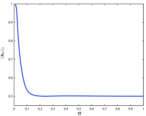
As the kernel scale parameterσdecreases, the kernel becomes less uniform thus increasing the possible variability in the data representation_kγ(y)_k2

2 and the covering number bound. In the case

of the bounded Gaussian kernel (6) we compute_|||Kσ|||2as a function of the kernel scale parameter

σwhich is illustrated in Figure 5.

5. Experiments

In this section, we demonstrate lowbow’s applicability to several text processing tasks, including text classification using nearest neighbor and support vector machines, text segmentation, and document visualization. All experiments use real world data.

5.1 Text Classification using Nearest Neighbor

We start by examining lowbow and its properties in the context of text classification using a nearest neighbor classifier. We report experimental results for the WebKB faculty vs. course task and the Reuters-21578 top ten categories (1 vs. all) using the standard mod-apte training-testing split. In the WebKB task we repeatedly sampled subsets for training and testing with equal positive and negative examples. In the Reuters task we randomly sampled subsets of the mod-apte split for training and testing data which resulted in unbalanced train and test sets containing more negative than positive examples. Sampling training sets of different sizes from the mod-apte split enabled us to examine the behavior of the classifiers as a function of the size of the training set.

0 0.1 0.2 0.3 0.4 0.5 0.6 0.7 0.8 0.9 1 0.5

0.6 0.7 0.8 0.9 1

PSfrag replacements

σ

|||

Kσ |||2

Figure 5: _|||Kσ|||2for the bounded Gaussian kernel (6) as a function of the kernel scale parameter

σ. The continuous 2-norm definition in (15) is approximated by 5 equally spaced samples for µ and 20 equally spaced samples for t.

points is rather arbitrary in our case and we did not find it critical to the nature of the experimental results. Throughout the experiments we used the bounded Gaussian kernel (6) and computed several alternatives for the kernel scale parameterσand chose the best one. While not entirely realistic, this setting enables us to examine lowbow’s behavior in the optimistic scenario of being able to find the best scale parameter. The next section includes similar text classification experiments using SVM that explore further the issue of automatically selecting the scale parameterσ.

Figure 6 (top) displays results for nearest neighbor classification using the Fisher geodesic dis-tance on the WebKB data. The left graph is a standard train-set size vs. test set error rate comparing the bow geodesic (lowbow withσ_→∞) (dashed) and the lowbow geodesic distance. The right graph displays the dependency of the test set error rate on the scale parameter indicating an opti-mal scale at aroundσ=0.2 (for repeated samplings of 500 training examples). In both cases, the performances of standard bow techniques such as tf cosine similarity or Euclidean distance were significantly inferior (20-40% higher error rate) than the Fisher geodesic distances and as a result are not displayed.

Figure 6 (bottom) displays test set error rates for the Reuters-21578 task. The 10 rows in the table indicate the classification task of identifying each of the 10 most popular classes in the Reuters collection. The columns represent varying training set sizes sampled from the mod-apte split. The lowbow geodesic distance for an intermediate scale is denoted by err1and forσ→∞is denoted by

err2. Tf-cosine similarity and Euclidean distance for bow are denoted by err3and err4.

The experiments indicate that lowbow geodesic clearly outperforms, for most values ofσ, the standard tf-cosine similarity and Euclidean distance for bow (represented by err3,err4). In addition

200 250 300 350 400 450 500 0.095

0.1 0.105 0.11 0.115 0.12 0.125 0.13

t siz e

t se

t e

rr

0 0.2 0.4 0.6 0.8 1 1.2 1.4 1.6 1.8 2

0.095 0.1 0.105 0.11 0.115 0.12 0.125

!#"$&%"'()*'",+*-$*./"10"$ 234

2

4

3

2

35

5

or r

6

23

Train Size=100 Train Size=200 Train Size=400

class err1 err2 err3 err4 err1 err2 err3 err4 err1 err2 err3 err4

1 9.9 10.6 11.2 11.0 8.1 9.7 8.2 10.7 6.7 7.3 11.2 9.0

2 11.6 12.8 17.6 22.4 9.4 9.7 17.6 19.9 7.9 7.8 17.2 17.9

3 6.8 7.6 6.9 12.9 5.8 7.2 7.8 16.9 5.4 5.3 10.2 12.6

4 5.6 6.5 6.5 5.5 4.8 4.8 7.1 7.0 4.5 4.7 8.5 7.5

5 6.6 6.2 9.0 11.4 5.7 6.8 6.7 10.3 5.0 5.6 5.8 7.4

6 5.7 5.8 5.8 10.8 5.2 5.3 5.3 10.0 4.8 5.4 5.6 11.3

7 4.2 5.1 7.0 12.9 4.2 4.3 7.9 9.0 3.9 4.3 5.8 7.5

8 3.0 3.2 4.7 7.6 3.0 3.3 3.4 3.4 2.6 2.9 3.2 3.9

9 2.8 4.0 4.9 7.9 3.1 3.0 6.4 2.8 2.9 3.2 4.7 5.1

10 2.7 2.9 3.6 2.6 2.6 3.0 5.8 3.1 2.3 2.6 3.7 2.2

Figure 6: Experimental test set error rates for WebKB course vs. faculty task (top) and Reuters top 10 classes using samples from mod-apte split (bottom). err1is obtained using the lowbow

geodesic distance with the optimal kernel scale. err2–err4denote using geodesic distance,

information using the lowbow framework to improve on global bow models. The next section describes similar experiments using SVM on the RCV1 data set which include automatic selection of the scale parameterσ.

5.2 Text Classification using Support Vector Machine

We extended our WebKB and Reuters-21578 text classification experiments to the more recently released and larger RCV1 data set (Lewis et al., 2004). In particular, we focused on the 1 vs. all classification tasks for topics that correspond to leaf nodes in the topic hierarchy and contain no less than 5000 documents. This results in a total of 43 topic codes displayed in Table 1. For further description of the topic hierarchy of the RCV1 data set refer to Lewis et al. (2004).

In our experiments we examined the classification performance of SVM with the Fisher diffu-sion kernel for bow (Lafferty and Lebanon, 2005) and its corresponding product verdiffu-sion for lowbow (10) (which reverts to the kernel of Lafferty and Lebanon (2005) forσ_→∞). Our experiments vali-date the findings in Lafferty and Lebanon (2005) which indicate a significantly poorer performance for linear or RBF kernels. We therefore omit these results and concentrate on comparing the SVM performance for the kernel (10) using various values ofσ.

We report the classification performance of SVM using the kernel (10) for three different values ofσ: (i)σ_→∞represents the standard bow diffusion kernel of Lafferty and Lebanon (2005) (ii)σopt

represents the best performing scale parameter in terms of test set error rate, and (iii) ˆσoptrepresents

an automatically selected scale parameter based on minimizing the leave-one-out cross validation (loocv) train-set error estimate computed by the SVM-light toolkit. In case of ties, we pick theσ with the smallest value, thus favoring less local smoothing. The loocv estimate is computed at no extra cost and is a convenient way to adaptively estimateσopt. In all of our experiments below we

ignore the role of the diffusion time t in (10) and simply try several different values and choose the best one.

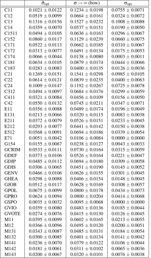
Table 1 reports the test set error rates and standard errors corresponding to the three scales ˆ

σopt,σ→∞,σopt for the selected RCV1 1 vs. all classification tasks. Notice that in general, the

lowbow ˆσoptsignificantly outperforms the standard bow approach. The performance ofσoptfurther

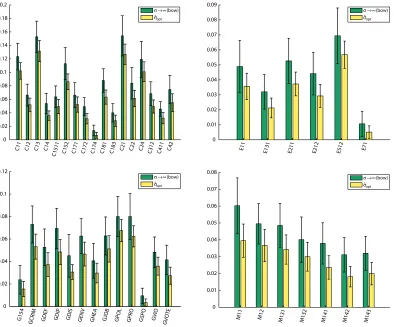
improves on that indicating that a more intelligent scale selection method could result in even lower error rates. Table 1 is also displayed graphically in Figure 8 for ˆσoptandσ→∞. Figure 7 shows the

corresponding train set loocv error rates and standard errors.

In our experiments, the sampling of the train and test sets were balanced, with equal number of positive and negative examples. Selections of the optimalσoptand the estimated ˆσoptwere done

based on the following set of possible values_{0.1,0.15,0.2,0.25,0.3,0.35,0.4,0.5,0.6,0.7,0.8,0.9, 1,2,4,10,100_}. In all the classification tasks, lowbow performs substantially better than bow. The error bars indicate one standard deviation from the mean, and support experimentally the assertion that lowbow has lower variance.

Figure 9 compares the performance of lowbow for ˆσopt, σ→∞, andσopt as a function of the

train set size (with the testing size being fixed as 200). As pointed out earlier, the performance of ˆ

σoptis consistently better than bow with some room for improvement represented by theσopt. 5.3 Dynamic Time Warping of Lowbow Curves

As presented in the previous sections, the lowbow framework normalizes the time interval[1,N]to

ˆ

σopt σ→∞(bow) σopt

C11 0.1021_±0.0122 0.1234_±0.0198 0.0755_±0.0071 C12 0.0519_±0.0099 0.0664_±0.0161 0.0324_±0.0072 C13 0.1316_±0.0156 0.1527_±0.0232 0.1008_±0.0088 C14 0.0359_±0.0070 0.0537_±0.0151 0.0190_±0.0050 C1511 0.0494_±0.0105 0.0636_±0.0163 0.0296_±0.0067 C152 0.0860_±0.0117 0.1129_±0.0239 0.0660_±0.0075 C171 0.0522_±0.0113 0.0662_±0.0185 0.0310_±0.0067 C172 0.0313_±0.0077 0.0491_±0.0134 0.0175_±0.0053 C174 0.0066_±0.0044 0.0138_±0.0080 0.0003_±0.0011 C181 0.0634_±0.0105 0.0879_±0.0174 0.0444_±0.0066 C183 0.0283_±0.0083 0.0400_±0.0135 0.0126_±0.0036 C21 0.1269_±0.0151 0.1541_±0.0298 0.0985_±0.0105 C22 0.0614_±0.0121 0.0839_±0.0235 0.0400_±0.0063 C24 0.1009_±0.0147 0.1192_±0.0267 0.0725_±0.0078 C312 0.0494_±0.0097 0.0684_±0.0176 0.0299_±0.0059 C411 0.0321_±0.0084 0.0456_±0.0109 0.0156_±0.0050 C42 0.0550_±0.0132 0.0745_±0.0211 0.0347_±0.0071 E11 0.0356_±0.0088 0.0489_±0.0174 0.0196_±0.0049 E131 0.0213_±0.0066 0.0320_±0.0115 0.0083_±0.0038 E211 0.0372_±0.0079 0.0526_±0.0151 0.0233_±0.0045 E212 0.0293_±0.0077 0.0441_±0.0142 0.0150_±0.0038 E512 0.0568_±0.0091 0.0694_±0.0186 0.0339_±0.0054 E71 0.0051_±0.0042 0.0106_±0.0084 0.0000_±0.0000 G154 0.0155_±0.0067 0.0238_±0.0127 0.0043_±0.0033 GCRIM 0.0533_±0.0111 0.0730_±0.0164 0.0315_±0.0059 GDEF 0.0373_±0.0106 0.0526_±0.0164 0.0221_±0.0047 GDIP 0.0485_±0.0112 0.0694_±0.0180 0.0309_±0.0058 GDIS 0.0306_±0.0065 0.0451_±0.0190 0.0145_±0.0052 GENV 0.0466_±0.0106 0.0626_±0.0155 0.0301_±0.0045 GHEA 0.0298_±0.0088 0.0406_±0.0154 0.0148_±0.0045 GJOB 0.0512_±0.0117 0.0628_±0.0169 0.0308_±0.0057 GPOL 0.0675_±0.0099 0.0800_±0.0178 0.0434_±0.0073 GPRO 0.0624_±0.0094 0.0800_±0.0204 0.0414_±0.0068 GSPO 0.0035_±0.0032 0.0095_±0.0068 0.0000_±0.0000 GVIO 0.0359_±0.0080 0.0483_±0.0136 0.0185_±0.0044 GVOTE 0.0274_±0.0076 0.0415_±0.0130 0.0126_±0.0045 M11 0.0395_±0.0099 0.0602_±0.0165 0.0213_±0.0055 M12 0.0366_±0.0096 0.0495_±0.0120 0.0200_±0.0051 M131 0.0343_±0.0087 0.0485_±0.0131 0.0184_±0.0054 M132 0.0300_±0.0085 0.0401_±0.0134 0.0141_±0.0042 M141 0.0236_±0.0070 0.0379_±0.0122 0.0106_±0.0044 M142 0.0181_±0.0061 0.0311_±0.0102 0.0065_±0.0036 M143 0.0200_±0.0067 0.0320_±0.0101 0.0076_±0.0038

0 0.02 0.04 0.06 0.08 0.1 0.1 2 0.1 4 0.1 6 0.1 8 0.2 C1 1 C1 2 C1 3 C1 4 C1 51 1 C1 52 C1 71 C1 72 C1 74 C1 81 C1 83 C2 1 C2 2 C2 4 C3 12 C4 11 C4 2

σ → ∞ (b o w ) σ^o p t

0 0.01 0.02 0.03 0.04 0.05 0.06 0.07 0.08 0.09

E11 _E131 _E211 _E212 _E512 E71

σ → ∞ (b o w ) σ^o p t

0 0.02 0.04 0.06 0.08 0.1 0.1 2 G1 54 GC RIM GD EF GD IP GD IS GE NV GH EA GJO B GP OL GP RO GS PO GV IO GV OT E

σ → ∞ (b o w )

σ^o p t

0 0.01 0.02 0.03 0.04 0.05 0.06 0.07 0.08 M1 1 M1 2 M1 31 M1 32 M1 41 M1 42 M1 43 σ → ∞ (b o w )

σ^ o p t

0 0.02 0.04 0.06 0.08 0.1 0.1 2 0.1 4 0.1 6 0.1 8 0.2 C1 1 C1 2 C1 3 C1 4 C1 511

C1 52 C1 71 C1 72 C1 74 C1 81 C1 83 C2 1 C2 2 C2 4 C3 12 C4 11 C4 2

σ → ∞ (b o w ) σ^o p t

0 0.01 0.02 0.03 0.04 0.05 0.06 0.07 0.08 0.09

E11 _E131 _E211 _E212 _E512 E71

σ → ∞ (b o w )

σ^o p t

0 0.02 0.04 0.06 0.08 0.1 0.1 2 G1 54 GC RIM GD EF GD IP GD IS GE NV GH EA GJO B GP OL GP RO GS PO GV IO GV OT E

σ → ∞ (b o w )

σ^o p t

0 0.01 0.02 0.03 0.04 0.05 0.06 0.07 0.08 M1 1 M1 2 M1 31 M1 32 M1 41 M1 42 M1 43 σ → ∞ (b o w )

σ^_{o p t}

100 150 200 250 300 350 400 450 500 550 600 0.08 0.1 0.12 0.14 0.16 0.18 0.2

0.22 C 21

σ → ∞ (b o w )

σ^_{o p t} σ

o p t

t r a in s e t s iz e

te st s e t e rr o r ra te

100 150 200 250 300 350 400 450 500 550 6 00

0.01 0.02 0.03 0.04 0.05 0.06 0.07

0.08 E 211

σ → ∞ (b o w ) σ^

o p t σ

o p t

t r a in s e t s iz e

te st s e t e rr o r ra te

100 150 200 250 300 350 400 450 500 550 600

0.02 0.03 0.04 0.05 0.06 0.07 0.08 0.09 0.1

0.11 G J O B

σ → ∞ (b o w )

σ^_{o p t}

σ_{o p t}

t r a in s e t s iz e

te st s e t e rr o r ra te

100 150 200 250 300 350 400 450 500 550 600

0 0.01 0.02 0.03 0.04 0.05 0.06

0.07 M 142

σ → ∞ (b o w )

σ^

o p t

σ_{o p t}

t r a in s e t s iz e

te st s e t e rr o r ra te

assumption of a product geometry, lowbow representations corresponding to different documents

y,z relate to each other by comparingγµ(y) toγµ(z) for all µ∈[0,1], for example as is the case in the integrated distance

d(γ(y),γ(z)) =

Z 1

0

d(γµ(y),γµ(z))dµ. (18)

This seems reasonable if the two documents y,z share a sequential progression of a similar

rate, after normalizing for document length. However, such an assumption seems too restrictive in general as documents of different nature such as news stories and personal webpages are unlikely to posses such similar sequential progression. This assumption also seems untrue to a lesser extent for two documents written by different authors who posses their own individual styles. Such cases can be modeled by introducing time-warping or re-parameterization functions that match the individual temporal domains of lowbow curves to a unique canonical parameterization. Before proceeding to discuss such re-parameterization in the context of lowbow curves we briefly review their use in speech recondition and functional data analysis.

In speech recognition such re-parameterization functions are used to align the time axes cor-responding to two speech signals uttered by different individuals or by the same individual under different circumstances. These techniques, commonly referred to as dynamic time warping (DTW) (Sakoe and Chiba, 1978), define the distance between two signals s,r as

d(s,r) = min

ι1,ι2∈I

Z

d(s(ι1(t)),r(ι2(t)))dt (19)

where I represent the class of smooth monotonic increasing bijectionsι:[0,1]_→[0,1]. Using dy-namic programming the discretized minimization problem corresponding to (19) can be efficiently computed, resulting in the wide spread use of DTW in the speech recognition community.

Similarly, such time parameterization techniques have been studied in functional data analysis under the name curve registration (Ramsay and Silverman, 2005). In contrast to dynamic time warping, curve registration is usually performed by an iterative procedure aimed at aligning salient features of the data and minimizing the post-alignment residual.

In contrast to the smoothness and monotonic nature of the re-parameterization class I in speech recognition and functional data analysis, it seems reasonable to allow some amount of discontinuity in lowbow re-parameterization. For example, while one document may posses a certain sequen-tial progression, a second document may reverse the appearance of some of the sequensequen-tial trends. Adjusting the original DTW definition of the re-parameterization family I we obtain the following modified characterization of the class of admissible re-parameterization.

Bijection Re-parameterizationι_∈I are a bijection from[0,1]onto itself.

Piecewise smoothness The re-parameterization functionsι_∈I are piecewise smooth and

mono-tonic, that is, given two partitions of[0,1]to sequences of disjoint intervals A1, . . . ,Ar with

∪Aj = [0,1] and B1, . . . ,Br with ∪Bj = [0,1]we have that for some permutation π over r items,ι: Aj→Bπ(j)is a smooth monotonic increasing bijection for all j=1, . . . ,r.

(Rubner et al., 2000) known as the Hungarian algorithm (Munkres, 1957), the minimization problem (19) over the class I described above may be computed efficiently.

We conducted a series of experiments examining the benefit in introducing dynamic time warp-ing or registration in text classification. Somewhat surpriswarp-ingly, addwarp-ing dynamic time warpwarp-ing or registration to lowbow classification resulted in only a marginal modification of the distances and consequently only a marginal improvement in classification performance. There are two reasons for this relatively minor effect introduced by the dynamic time warping. First, the RCV1 corpus for which these experiments were conducted consists of documents containing a fairly homogeneous semantic structure and presentation. As such, the curves can reasonably be compared by using in-tegrated distances or kernels without a need for re-parameterization. Second, the local smoothing inherent in the lowbow representation makes it fairly robust to some amount of temporal misalign-ment. In particular, by selecting the kernel scale parameter appropriately we are able to prevent unfortunate effects due to different sequential parameterizations. Although surprising, this is in-deed a positive result as it indicates that the lowbow representation is relatively robust to different time parameterization, at least when applied to documents sharing similar structure such as news stories in RCV1 corpus or webpages in the WebKB data set.

5.4 Text Segmentation

Text segmentation is the task of discovering topical boundaries inside documents, for example tran-scribed news-wire data. In general, this task is hard to accomplish using low order n-gram infor-mation. Most methods use a combination of longer range n-grams and other sequential features such as trigger pairs. Our approach in this section is not to carefully construct a state-of-the-art text segmentation system but rather to demonstrate the usefulness of the continuous lowbow representa-tion in this context. More informarepresenta-tion on text segmentarepresenta-tion and a recent exponential model-based approach may be found in Beeferman et al. (1999).

The boundaries between different text segments, by definition, separate document parts contain-ing different word distributions. In the context of lowbow curves, this would correspond to sudden dramatic shifts in the curve location. Due to the continuity of the lowbow curves, such sudden movements may be discovered by considering the gradient vector field ˙γµalong the lowbow curve. In addition to containing predictive information that can be used in segmentation models, the gra-dient enables effective visualization of the instantaneous change that is central to human-assisted segmentation techniques.

0 0.2 0.4 0.6 0.8 1 0.5

0.55 0.6 0.65 0.7 0.75 0.8 0.85

0

0.2

0.4

0.6

0.8

1.0

PSfrag replacements

.20

.40 0 0.2 0.4 0.6 0.8 1

0.85 0.9 0.95 1 1.05 1.1 1.15 1.2 1.25

0

0.19

0.41

0.65

0.75 0.91

PSfrag replacements

.20 .40

Figure 10: Velocity of the lowbow curve as a function of t. Left: five randomly sampled new stories of equal size (σ=0.08). Right: three successive RCV1 news articles of varying lengths (σ=0.065).

The first document was created by concatenating five randomly sampled news stories from the Wall Street Journal data set. To ensure that the different segments will be of equal length, we removed the final portions of the longer stories thus creating predetermined segment borders at

µ=0.2,0.4,0.6,0.8. The gradient norm_kγ˙µ(y)k2of this document is displayed in the the left panel

of Figure 10. Notice how the 4 equally spaced internal segment borders (displayed by the numbered circles in the figure), correspond almost precisely, to the local maxima of the gradient norm.

The second document, represents a more realistic scenario where the segments correspond to successive news stories of varying lengths. We created it by randomly picking three successive news articles from the RCV1 collection (document id: 18101, 18102 and 18103) and concatenating them into a single document. The two internal segment borders occur at µ=0.19 and µ=0.41 (the last story is obviously longer than the first two stories). The right panel of Figure 10 displays the gradient norm_kγ˙µk2 for the corresponding lowbow curve. The curve has five local maxima, with

the largest two local maxima corresponding almost precisely to the segment borders at µ=0.19 and µ=0.41. The three remaining local maxima correspond to internal segment boundaries within the third story. Indeed, the third news story begins with discussion of London shares and German stocks; it then switches to discuss French stocks at point µ=0.65 before switching again at µ=0.75 to talk about how the Bank of Japan’s quarterly corporate survey affects the foreign exchange. The story moves on at µ=0.95 to discuss statistics of today’s currencies and stock market. As with the different news story boundaries, the internal segment boundaries of the third story closely match the local maxima of the gradient norm.

−0.15 −0.1 −0.05 0 0.05 0.1 −0.15

−0.1 −0.05 0 0.05 0.1

0 0.19

0.41

1.0

−0.8 −0.6 −0.4 −0.2 0 0.2 0.4 0.6

−0.8 −0.6 −0.4 −0.2 0 0.2 0.4 0.6

0 0.19

0.41

1.0

Figure 11: 2D embeddings of the lowbow curve representing the three successive RCV1 stories (see text for more details) using PCA (left,σ=0.02) and MDS (right,σ=0.01).

text content. Such techniques for rapid document visualization and browsing are also illustrated in the next section.

Figure 11 shows the 2D projection of the lowbow curve for the three concatenated RCV1 stories mentioned above. To embed the high dimensional curve in two dimensions we used principal com-ponent analysis (PCA) (left panel) and multidimensional scaling using the Fisher geodesic distance (right). The blue crosses indicate the positions of the sampled points in the low dimensional em-bedding while the red circles correspond to the segment boundaries of the three RCV1 documents. In both figures,_{γµ1(y), . . . ,γµk(y)}are naturally grouped into three clusters, indicating the presence of three different segments. The distance between successive points near the segment boundaries is relatively large which demonstrates the high speed of the lowbow curve at these points (compare it with the gradient norm in right panel of Figure 10).

5.5 Text Visualization

We conclude the experiments with a text visualization demonstration based on the current journal article. Visualizing this document has the added benefit that the reader is already familiar with the text, hopefully having read it carefully thus far. Additional visualization applications of the lowbow framework may be found in Mao et al. (2007).

The gradient norm k˙γ(t)_k2 of the lowbow curve of this paper is displayed in Figure 12. The

0 0.2 0.4 0.6 0.8 1 0.7

0.8 0.9

1 1.1 1.2 1.3 1.4

0 (1)

0.085 (2)

0.23 5 (3 ) 0.3 7 (4)

0.46 (4.2)

0.5 45 (5 ) 0.665 (5 .3 ) 0.7 7 (5 .4)

0.865 (6)

0.9 5 5 (A p p e n d ix )

1.0 0.17

0.61 (5 .2)

0.9 2 (7 )

Figure 12: Velocity of the lowbow curve computed for this paper as a function of µ (σ=0.04). Abstract, references and Section 5.5 are excluded from curve generation. The marks indicate the beginning of each section that are identified by numbers in parentheses, for example, Section 2 begins at µ=0.085.

Figure 13 depicts 2D projections of the lowbow curve corresponding to Sections 5.1–5.4 (sec-tion boundaries occurring at µ=_{0.2,0.38,0.72_}) using PCA (left) and MDS (right) based on Fisher geodesic distance. As previously demonstrated, the lowbow curve nicely reveals three clus-ters corresponding to the different subsections with the exception of not distinguishing between the nearest neighbor and SVM experiments. Using interactive graphics it is possible to extract more information from the lowbow curves by examining the 3D PCA projection, displayed in Figure 14. The dense clustering of the points at the beginning of the 2D curve is separated in the 3D figure, however, there is no way to separate the crossing at the end of the curve in both 3D and 2D.

6. Related Work

The use of n-gram and bow has a long history in speech recognition, language modeling, informa-tion retrieval and text classificainforma-tion. Recent monographs surveying these areas are Jelinek (1998), Manning and Schutze (1999), and Baeza-Yates and Ribeiro-Neto (1999). In speech recognition and language modeling n-grams are used typically with n=1,2,3. In classification, on the other hand, 1-grams or bow are the preferred option. While some attempts have been made to use bi-grams and tri-grams in classification as well as to incorporate richer representations, the bow representation is still by far the most popular.