Manifold Regularization and Semi-supervised Learning: Some Theoretical Analyses

Manifold Regularization and Semi-supervised Learning:

Some Theoretical Analyses

Partha Niyogi∗

Departments of Computer Science, Statistics University of Chicago

1100 E. 58th Street, Ryerson 167 Hyde Park, Chicago, IL 60637, USA

Editor: Zoubin Ghahramani

Abstract

Manifold regularization (Belkin et al., 2006) is a geometrically motivated framework for machine learning within which several semi-supervised algorithms have been constructed. Here we try to provide some theoretical understanding of this approach. Our main result is to expose the natural structure of a class of problems on which manifold regularization methods are helpful. We show that for such problems, no supervised learner can learn effectively. On the other hand, a manifold based learner (that knows the manifold or “learns” it from unlabeled examples) can learn with relatively few labeled examples. Our analysis follows a minimax style with an emphasis on finite sample results (in terms of n: the number of labeled examples). These results allow us to properly interpret manifold regularization and related spectral and geometric algorithms in terms of their potential use in semi-supervised learning.

Keywords: semi-supervised learning, manifold regularization, graph Laplacian, minimax rates

1. Introduction

The last decade has seen a flurry of activity within machine learning on two topics that are the subject of this paper: manifold method and semi-supervised learning. While manifold methods are generally applicable to a variety of problems, the framework of manifold regularization (Belkin et al., 2006) is especially suitable for semi-supervised applications.

Manifold regularization provides a framework within which many graph based algorithms for semi-supervised learning have been derived (see Zhu, 2008, for a survey). There are many things that are poorly understood about this framework. First, manifold regularization is not a single algo-rithm but rather a collection of algoalgo-rithms. So what exactly is “manifold regularization”? Second, while many semi-supervised algorithms have been derived from this perspective and many have en-joyed empirical success, there are few theoretical analyses that characterize the class of problems on which manifold regularization approaches are likely to work. In particular, there is some confusion on a seemingly fundamental point. Even when the data might have a manifold structure, it is not clear whether learning the manifold is necessary for good performance. For example, recent results (Bickel and Li, 2007; Lafferty and Wasserman, 2007) suggest that when data lives on a low dimen-sional manifold, it may be possible to obtain good rates of learning using classical methods suitably

adapted without knowing very much about the manifold in question beyond its dimension. This has led some people (e.g., Lafferty and Wasserman, 2007) to suggest that manifold regularization does not provide any particular advantage.

What is particularly missing in the prior research so far is a crisp theoretical statement which shows the benefits of manifold regularization techniques quite clearly. This paper provides such a theoretical analysis, and explicates the nature of manifold regularization in the context of semi-supervised learning. Our main theorems (Theorems 2 and 4) show that there can be classes of learn-ing problems on which (i) a learner that knows the manifold (alternatively learns it from large (in-finite) unlabeled data via manifold regularization) obtains a fast rate of convergence (upper bound) while (ii) without knowledge of the manifold (via oracle access or manifold learning), no learning scheme exists that is guaranteed to converge to the target function (lower bound). This provides for the first time a clear separation between a manifold method and alternatives for a suitably chosen class of problems (problems that have intrinsic manifold structure). To illustrate this conceptual point, we have defined a simple class of problems where the support of the data is simply a one dimensional manifold (the circle) embedded in an ambient Euclidean space. Our result is the first of this kind. However, it is worth emphasizing that this conceptual point may also obtain in far more general manifold settings. The discussion of Section 2.3 and the theorems of Section 3.2 provide pointers to these more general results that may cover cases of greater practical relevance.

The plan of the paper: Against this backdrop, the rest of the paper is structured as follows. In Section 1.1, we develop the basic minimax framework of analysis that allows us to compare the rates of learning for manifold based semi-supervised learners and fully supervised learners. Following this in Section 2, we demonstrate a separation between the two kinds of learners by proving an upper bound on the manifold based learner and a lower bound on any alternative learner. In Section 3, we take a broader look at manifold learning and regularization in order to expose some subtle issues around these subjects that have not been carefully considered by the machine learning community. This section also includes generalizations of our main theorems of Section 2. In Section 4, we consider the general structure that learning problems must have for semi-supervised approaches to be viable. We show how both the classical results of Castelli and Cover (1996, one of the earliest known examples of the power of semi-supervised learning) and the recent results of manifold regularization relate to this general structure. Finally, in Section 5 we reiterate our main conclusions.

1.1 A Minimax Framework for Analysis

A learning problem is specified by a probability distribution p on X_×Y according to which labelled

examples zi= (xi,yi)pairs are drawn and presented to a learning algorithm (estimation procedure).

We are interested in an understanding of the case in which X =RD, Y _⊂Rbut pX (the marginal

distribution of p on X ) is supported on some submanifold

M

_⊂X . In particular, we are interested

in understanding how knowledge of this submanifold may potentially help a learning algorithm. To this end, we will consider two kinds of learning algorithms:

1. Algorithms that have no knowledge of the submanifold

M

_{but learn from(xi,yi) pairs in a}

purely supervised way.

2. Algorithms that have perfect knowledge of the submanifold. This knowledge may be acquired

essentially infinite number of them. Such a learner may be viewed as a semi-supervised learner.

Our main result is to elucidate the structure of a class of problems on which there is a difference in the performance of algorithms of Type 1 and 2.

Let

P

_{be a collection of probability distributions p and thus denote a class of learning problems.}

For simplicity and ease of comparison with other classical results, we place some regularity

con-ditions on

P

. Every p_∈

P

is such that its marginal pX has support on a k-dimensional manifold

M

_{⊂X . Different p’s may have different supports. For simplicity, we will consider the case where}

pX is uniform on

M

: this corresponds to a situation in which the marginal is the most regular.

Given such a

P

we can naturally define the class

P

_M to be

P

_M =_{p_∈P_|pX is uniform on

M

}.

Clearly, we have

P

_=∪M

P

_M.

Consider p∈

P

_{M. This denotes a learning problem and the regression function mpis defined as}

mp(x) =E[y|x]when x∈

M

.

Note that mp(x)is not defined outside of

M

. We will be interested in cases when mp belongs to

some restricted family of functions HM (for example, a Sobolev space). Thus assuming a family

HM is equivalent to assuming a restriction on the class of conditional probability distributions p(y|x)

where p_∈

P

_{. For simplicity, we will assume the noiseless case where p(y|x) is either 0 or 1 for every}

x and every y, that is, there is no noise in the Y space.

Since X_\

M

has measure zero (with respect to pX), we can define mp(x)to be anything we want

when x_∈X_\

M

_{. We define mp(x) =0 when x∈/}

M

_.

For a learning problem p, the learner is presented with a collection of labeled examples _{zi=

(xi,yi),i=1, . . . ,n}where each zi is drawn i.i.d. according to p. A learning algorithm A maps the

collection of data z= (z1, . . . ,zn)into a function A(z). Now we can define the following minimax

rate (for the class

P

) as

R(n,

P

) =inf

A sup_p∈PEz||A(z)−mp||L2(pX).

This is the best possible rate achieved by any learner that has no knowledge of the manifold

M

. We

will contrast it with a learner that has oracle access endowing it with knowledge of the manifold. To

begin, note that since

P

=_∪M

P

M, we see that

R(n,

P

) =inf

A sup_{M p}sup_∈P M

Ez||A(z)−mp||L2_(p

X).

Now a manifold based learner A′is given a collection of labeled examples z= (z1, . . . ,zn) just

like the supervised learner. However, in addition, it also has knowledge of

M

(the support of the

unlabeled data). It might acquire this knowledge through manifold learning or through oracle access

(the limit of infinite amounts of unlabeled data). Thus A′ maps(z,

M

)into a function denoted by

A′(z,

M

). The minimax rate for such a manifold based learner for the class

P

_M is given by

inf

A′ sup

p∈PM

Ez||A′(z,

M

)−mp||L2_(p

Taking the supremum over all possible manifolds (just as in the supervised case), we have

Q(n,

P

) =sup

M

inf

A′ _psup

∈P_M

Ez||A′−mp||L2_(p

X).

1.2 The Manifold Assumption for Semi-supervised Learning

So the question at hand is: for what class of problems

P

with the structure as described above, might

one expect a gap between R(n,

P

)and Q(n,

P

). This is a class of problems for which knowing the

manifold confers an advantage to the learner.

There are two main assumptions behind the manifold based approach to semi-supervised learn-ing. First, one assumes that the support of the probability distribution is on some low dimensional manifold. The motivation behind this assumption comes from the intuition that although natural data in its surface form lives in a high dimensional space (speech, image, text, etc.), they are often generated by systems with much fewer underlying degrees of freedom and therefore have lower intrinsic dimensionality. This assumption and its corresponding motivation has been articulated many times in papers on manifold methods (see Roweis and Saul, 2000, for example). Second, one assumes that the underlying target function one is trying to learn (for prediction) is smooth with respect to this underlying manifold. A smoothness assumption lies at the heart of many machine learning methods including especially splines (Wahba, 1990), regularization networks (Evgeniou et al., 2000), and kernel based methods (using regularization in reproducing kernel Hilbert spaces; Sch¨olkopf and Smola, 2002). However, smoothness in these approaches is typically measured in the ambient Euclidean space. In manifold regularization, a geometric smoothness penalty is instead imposed.

Thus, for a manifold M, letφ1,φ2, . . . ,be the eigenfunctions of the manifold Laplacian (ordered

by frequency). Then, mp(x)may be expressed in this basis as mp=∑iαiφior

mp=sign(

∑

i

αiφi)

where theαi’s have a sharp decay to zero.

Against this backdrop, one might now consider manifold regularization to get some better under-standing of when and why it might be expected to provide good semi-supervised learning. First off, it is worthwhile to clarify what is meant by manifold regularization. The term “manifold regulariza-tion” was introduced by Belkin et al. (2006) to describe a class of algorithms in which geometrically motivated regularization penalties were used. One unifying framework adopts a setting of Tikhonov regularization over a Reproducing Kernel Hilbert Space of functions to yield algorithms that arise as special cases of the following:

ˆ

f =arg min

f∈HK 1 n

n

∑

i=1

V(f(xi),yi) +γA||f||2K+γI||f||2I. (1)

Here K : X_×X_→Ris a p.d. kernel that defines a suitable RKHS (HK) of functions that are

ambi-ently defined. The ambient RKHS norm_||f_||K and an “intrinsic norm”||f||I are traded-off against

each other. Intuitively the intrinsic norm _||f_||I penalizes functions by considering only fM the

restriction of f to

M

and essentially considering various smoothness functionals. Since the

express fM =∑iαiφiin this basis and consider constraints on the coefficients.

Remarks:

1. Various choices of _||f_||2_I include: (i) iterated Laplacian given by R_M f(∆i_{f) =∑jα}2

jλij, (ii)

heat kernel given by∑jetλjα2j, and (iii)band limiting given by||f||2I =∑iµiα2i where µi=∞

for all i>p.

2. The loss function V can vary from squared loss to hinge loss to the 0–1 loss for classification giving rise to different kinds of algorithmic procedures.

3. While Equation 1 is regularization in the Tikhonov form, one could consider other kinds of model selection principles that are in the spirit of manifold regularization. For example, the method of Belkin and Niyogi (2003) is a version of the method of sieves that may be inter-preted as manifold regularization with bandlimited functions where one allows the bandwidth to grow as more and more data becomes available.

4. The formalism provides a class of algorithms A′ that have access to labeled examples z and

the manifold

M

from which all the terms in the optimization of Equation 1 can be computed.

Thus A′(z,

M

) =f .ˆ

5. Finally it is worth noting that in practice when the manifold is unknown, the quantity_{R ||}f_||2_I =

M f(∆if)is approximated by collecting unlabeled points xi∈

M

, making a suitable nearest

neighbor graph with the vertices identified with the unlabeled points, and regularizing the function using the graph Laplacian. The graph is viewed as a proxy for the manifold and in this sense, many graph based approaches to semi-supervised learning (see Zhu, 2008, for review) may be accommodated within the purview of manifold regularization.

The point of these remarks is that manifold regularization combines the perspective of kernel based methods with the perspective of manifold and graph based methods. It admits a variety of different algorithms that incorporate a geometrically motivated complexity penalty. We will later demonstrate (in Section 3) one such canonical algorithm for the class of learning problems considered in Section 2 of this paper.

2. A Prototypical Example: Embeddings of the Circle into Euclidean Space

In this section, we will construct a class of learning problems

P

_{that have manifold structure}

P

=

∪M

P

M and demonstrate a separation between R(n,

P

)and Q(n,

P

). For simplicity, we will show a

specific construction where every

M

considered is a different embedding of the circle into Euclidean

space. In particular, we will see that R(n) =Ω(1) while limn→∞Q(n) =0 at a fast rate. Thus the learner with knowledge of the manifold learns easily while the learner with no such knowledge cannot learn at all.

Letφ: S1_{→X be an isometric embedding of the circle into a Euclidean space. Now consider} the family of such isometric embeddings and let this be the family of one-dimensional submanifolds

that we will deal with. Thus each

M

_⊂X is of the form

M

=φ(S1)for someφ.

Let H_S1 be the set of functions defined on the circle that take the value+1 on half the circle and

−1 on the other half. Thus in local coordinates (θdenoting the coordinate of a point in S1), we can

HS1 ={hα: S1→R|hα(θ) =sign(sin(θ+α));α∈[0,2π)}.

Now for each

M

=θ(S1)we can define the class HM as

HM ={h :

M

→R|h(x) =hα(φ−1(x))for some hα∈HS1}. (2)

This defines a class of regression functions (also classification functions) for our setting.

Cor-respondingly, in our noiseless setting, we can now define

P

_M as follows. For each, h_∈HM, we

can define the probability distribution p(h)on X_×Y by letting the marginal p(_Xh)be uniform on

M

and the conditional p(h)(y_|x)be a probability mass function concentrated on two points y= +1 and

y=₋1 such that

p(h)(y= +1_|x) =1_⇐⇒h(x) = +1

Thus

P

_M =_{p(h)_|h_∈HM}

In our setting, we can therefore interpret the learning problem as an instantiation either of re-gression or of classification based on our interest.

Now that

P

_{M is defined, the set}

P

=_∪M

P

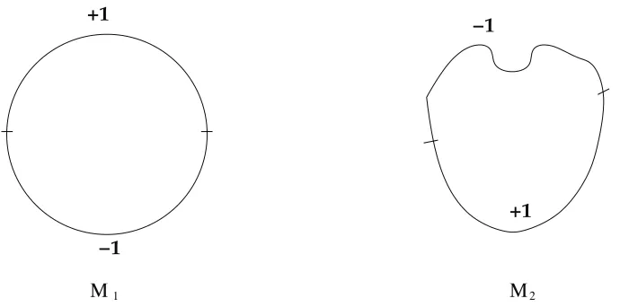
_{M follows naturally. A picture of the situation is}

shown in Figure 1.

Remark 1 Recall that many machine learning methods (notably splines and kernel methods)

con-struct classifiers from spaces of smooth functions. The Sobolev spaces (see Adams and Fournier, 2003) are spaces of functions whose derivatives up to a certain order are square integrable. These spaces arise in theoretical analysis of such machine learning methods and it is often the case that predictors are chosen from such spaces or regression functions are assumed to be in such spaces depending on the context of the work. For example, Lafferty and Wasserman (2007) make precisely such an assumption. In our setting, note that HS1 and correspondingly H_M as defined above is not

itself a Sobolev space. However, it is obtained by thresholding functions in a Sobolev space. In particular, we can write

HS1 ={sign(h)|h=αφ+βψ}

where φ(θ) =sin(θ) and ψ(θ) = cos(θ) are eigenfunctions of the Laplacian ∆_S1 on the circle.

These are the eigenfunctions corresponding toλ=1 and define the corresponding two dimensional eigenspace. More generally one could consider a family of functions obtained by thresholding functions in a Sobolev space of any chosen order and clearly H_S1 is contained in any such family.

+1

−1

+1 −1

Μ1 Μ2

Figure 1: Shown are two embeddings of M1 and M2of the circle in Euclidean space (the plane in

this case). The two functions, one from M1_→Rand the other from M2_→Rare denoted

by labelings+1,₋1 correspond to half circles shown.

2.1 Upper Bound on Q(n,

P

)

Let us begin by noting that if the manifold

M

is known, the learner knows the class

P

_M. The

learner merely needs to approximate one of the target functions in HM. It is clear that the space HM

is a family of 0 – 1 valued functions whose VC-dimension is 2. Therefore, an algorithm that does

empirical risk minimization over the class HM will yield an upperbound of O(

q

log(n)

n )by the usual

arguments. Therefore the following theorem is obtained.

Theorem 2 Following the notation of Section 1, let HM be the family of functions defined by

Equa-tion 2 and

P

_{be the corresponding family of learning problems. Then the learner with knowledge of}

the manifold converges at a fast rate given by

Q(n,

P

)_≤2

r

3 log(n)

n

and this rate is optimal. Thus every problem in this class P can be learned efficiently.

Remark 3 If the class HM is a a parametric family of the form∑ip=1αiφi where φi are the eigen-functions of the Laplacian, one obtains the same parametric rate. Similarly, if the class HM is a

ball in a Sobolev space of appropriate order, suitable rates on the family may be obtained by the usual arguments.

2.2 Lower Bound on R(n,

P

)

We now prove the following.

Theorem 4 Let

P

=_∪M

P

M where each

M

=φ(S1)is an isometric embedding of the circle into

given by the construction in the previous section. Then

R(n,

P

) =inf

A sup_p∈PEz||A(z)−mp||L2(pX)=Ω(1)

Thus, it is not the case that every problem in the class

P

_{can be learned efficiently. In other words,}

for every n, there exists a problem in

P

that requires more than n examples.

We provide the proof below. A specific role in the proof is played by a construction (Construc-tion 1 later in the proof) that is used to show the existence of a family of geometrically structured learning problems (probability measures) that will end up becoming unlearnable as a family. Proof Given n, choose a number d=2n. Following Construction 1, there exist a set (denoted

by

P

_{d ⊂}

P

) of 2d _{probability distributions that may be defined. Our proof uses the probabilistic}

method. We show that there exists a universal constant K (independent of n) such that

∀A, 1

2d

∑

p_∈Pd

Ez||A(z)−mp||L2_(p

X)≥K

from which we conclude that

∀A,sup

p∈Pd

Ez||A(z)−mp||L2_(p

X)≥K

Since

P

_d⊂

P

_{, the result follows.}

To begin, consider a p_∈

P

. Let z= (z1, . . . ,zn) be a set of i.i.d. examples drawn according to

p. Note that this is equivalent to drawing x= (x1, . . . ,xn) i.i.d. according to pX and for each xi,

drawing yi according to p(y|xi). Since the conditional p(y|x)is concentrated on one point, the yi’s

are deterministically assigned. Accordingly, we can denote this dependence by writing z=zp(x).

Now consider

Ez||A(z)−mp||L2_(p

X).

This is equal to Z

ZndP(z)||A(z)−mp||L

2_(p

X)= Z

Xnd p

n

X(x)||A(zp(x))−mp||L2_(p

X).

(To clarify notation, we observe that d pn_X is the singular measure on Xnwith support on

M

n_which

is the natural product measure corresponding to the distribution of n data points x1, . . . ,xn drawn

i.i.d. with each xidistributed according to pX.) The above in turn is lowerbounded by

≥

n

∑

l=0 Z

x∈Sl

d pn_X(x)_||A(zp(x))−mp||L2_(p

X)

where

Sl={x∈Xn|exactly l segments contain data and links do not}.

More formally,

Now we concentrate on lowerboundingR_x∈Sld pn_X(x)_||A(zp(x))−mp||L2_(p

X). Using the fact that

pX is uniform, we have that d pnX(x) =cd(x) (where c is a normalizing constant and d(x) is the

Lebesgue measure or volume form on the associated product space) and therefore Z

x_∈Sl

d pn_X(x)_||A(zp(x))−mp||L2_(p

X)= Z

x_∈Sl

cd(x)_||A(zp(x))−mp||L2_(p

X).

Thus, we have

Ez||A(z)−mp||L2_(p

X)≥

n

∑

l=0 Z

x∈Sl

cd(x)_||A(zp(x))−mp||L2_(p

X). (3)

Now we see that

[l]1

2d

∑

p∈Pd

Ez||A(zp(x))−mp||L2_(p

X)≥ 1

2d

∑

p∈Pd

n

∑

l=0 c

Z

x∈Sl

d(x)_||A₋mp||

≥

n

∑

l=0 c

Z

x∈Sl 1

2d

∑

p

||A₋mp|| !

d(x).

By Lemma 5, we see that for each x_∈Sl, we have

1

2d

∑

p

||A₋mp|| ≥(1−α−β)

d₋n 4d

from which we conclude that

1

2d

∑

p

Ez||A(z)−mp||L2_(p

X)≥(1−α−β)

d₋n 4d

n

∑

l=0 Z

x∈Sl

cd(x).

Now we note that

n

∑

l=0 Z

x∈Sl

cd(x) =Prob(x_∩B=/0)_≥(1₋β)n.

Therefore,

sup

p

Ez||A(z)−mp||L2_(p

X)≥(1−α−β)

d−n

4d (1−β)

n

≥(1₋α₋β)1 8(1−β)

n_{. (4)}

Sinceαandβ(and for that matter, d) are in our control, we can choose them to make the

right-hand side of Inequality 4 greater than some constant. This proves our theorem.

We now construct a family of intersecting manifolds such that given two points on any manifold in this family, it is difficult to judge (without knowing the manifold) whether these points are near or far in geodesic distance. The class of learning problems consists of probability distributions p

such that pX is supported on some manifold in this class. This construction plays a central role in

the proof of the lower bound.

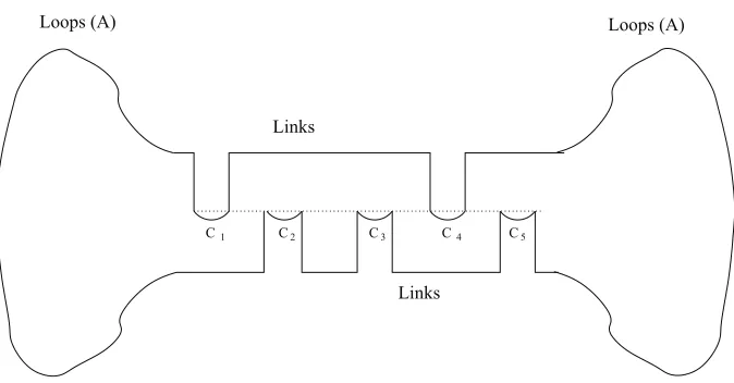
Construction 1. Consider a set of 2d manifolds where each manifold has a structure shown in Figure 2. Each manifold has three disjoint subsets: A (loops), B (links), and C (chain) such that

Loops (A) Loops (A)

C1 C2 C3 C4 C5

Links

Links

Figure 2: Figure accompanying Construction 1.

The chain C consists of d segments denoted by C1,C2, . . . ,Cdsuch that C=∪Ci. The links connect

the loops to the segments as shown in Figure 2 so that one obtains a closed curve corresponding to

an embedding of the circle intoRD. For each choice S_{⊂ {}1, . . . ,d_}one constructs a manifold (we

can denote this by

M

_S) such that the links connect Ci (for i∈S) to the “upper half” of the loop and

they connect Cj (for j∈ {1, . . . ,d} \S) to the “bottom half” of the loop as indicated in the figure.

Thus there are 2d manifolds altogether where each

M

_S differs from the others in the link structure

but the loops and chain are common to all, that is,

A_∪C_{⊂ ∩}S

M

S.

For manifold

M

_S, let

l(A)

l(

M

_S) = Z

A

p(_XS)(x)dx=αS

where p(_XS)is the probability density function on the manifold

M

_S. Similarly

l(B)

l(

M

_S) = Z

B

p(_XS)(x)dx=βS

and

l(C)

l(

M

_S)=

Z

C

p(_XS)(x)dx=γS.

It is easy to check that one can construct these manifolds so that

βS≤β;γS≥γ.

Thus for each manifold

M

_S, we have the associated class of probability distributions

P

_M

S. These

are used in the construction of the lower bound. Now for each such manifold

M

_S, we pick one

probability distribution p(S)_∈

P

_M

S such that for every k∈S, we have

and for every k∈ {1, . . . ,d} \S, we have

For all k_{∈ {}1, . . . ,d_{} \}S,p(S)(y=₋1_|x) =1 for all x_∈Ck.

Furthermore, the p(S)_{are all chosen so that the associated conditionals p}(S)_{(y= +1|x)agree on}

the loops, that is, for any S,S_{′ ∈ {}1, . . . ,d_},

p(S)(y= +1_|x) =p(S′)(y= +1_|x)for all x_∈A

This defines 2d different probability distributions that satisfy for each p: (i) the support of the

marginal pX includes A∪C, (ii) the support of pX for different p have different link structures (iii)

the conditionals p(y_|x)disagree on the the chain. We now prove the following technical lemma that

proves an inequality that holds when the data only lives on the segments and not on the links that constitute the embedded circle of Construction 1. This inequality is used in the proof of Theorem 4.

Lemma 5 Let x_∈Sl be a collection of n points such that no point belongs to the links and exactly

l segments contain at least one point.

1

2d

∑

p∈Pd

||A(zp(x))−mp||L2_(p

X)≥(1−α−β)

d₋n

4d .

Proof Since x_∈Sl, there are d−l segments of the chain C such that no data is seen from them.

We let A(zp(x))be the function hypothesized by the learner on receiving the data set zp(x). We

begin by noting that the family

P

_d may be naturally divided into 2l subsets in the following way.

Following the notation of Construction 1, recall that every element of

P

_d may be identified with

a set S_{⊂ {}1, . . . ,d_}. We denote this element by p(S)_{. Now let L denote the set of indices of the}

segments Ci that contain data, that is,

L=_{i_|Ci∩x6=/0}.

Then for every subset D_⊂L, we have

P

_D=_{p(S)_∈

P

_d|S_∩L=D_}.

Thus all the elements of

P

_{Dagree in their labelling of the segments containing data but disagree}

in their labelling of segments not containing data. Clearly there are 2l possible choices for D and

each such choice leads to a family containing 2dl probability distributions. Let us denote these 2l

families by

P

_1through

P

₂l.

Consider

P

_i. By construction, for all probability distributions p,q_∈

P

_i, we have that zp(x) =

zq(x). Let us denote this by zi(x), that is, zi(x) =zp(x)for all p∈

P

i.

Now f =A(zi(x))is the function hypothesized by the learner on receiving the data set zi(x).

For any p_∈

P

and any segment ck, we say that p “disagrees” with f on ck if|f(x)mp(x)| ≥1 on a

majority of ck, that is, Z

A

pX(x)≥

Z

ck\A

pX(x)

where A=_{x_∈ck||f(x)mp(x)| ≥1}. Therefore, if f and p disagree on ck, we have

Z

ck

(f(x)₋mp(x))2pX(x)≥

1 2 Z

ck

pX(x)≥

1

It is easy to check that for every choice of j unseen segments, there exists a p∈

P

_{i such that p}

disagrees with f on each of the chosen segments. Therefore, for such a p, we have

||(A(zp(x))−mp||2_L2_(p

X)≥ 1 2 j

d(1−α−β).

Counting all the 2dl elements of

P

_{i based on the combinatorics of unseen segments, we see (using}

the fact that||A(zp(x))−mp|| ≥ q

1 2

j

d(1−α−β)≥

1 2

j

d(1−α−β))

∑

p∈Pi

||A(xp(x)−mp|| ≥ d₋l

∑

j=0

d₋l j

1 2 j

d(1−α−β) =2

d−l₍₁

−α−β)d−l

4d .

Therefore, since l_≤n, we have

2l

∑

i=1p

∑

∈Pi

||A(xp(x))−mp|| ≥2d(1−α−β)

d₋n

4d .

2.3 Discussion

Thus we see that knowledge of the manifold can have profound consequences for learning. The proof of the lower bound reflects the intuition that has always been at the root of manifold based methods for semi-supervised learning. Following Figure 2, if one knows the manifold, one sees that

C1 and C4 are “close” while C1 and C3 are “far.” But this is only one step of the argument. We

must further have the prior knowledge that the target function varies smoothly along the manifold and so “closeness on the manifold” translates to similarity in function values (or label probabilities). However, this closeness is not obvious from the ambient distances alone. This makes the task of the learner who does not know the manifold difficult: in fact impossible in the sense described in Theorem 4.

Some further remarks are in order. These provide an idea of the ways in which our main the-orems can be extended. Thus we may appreciate the more general circumstances under which we might see a separation between manifold methods and alternative methods.

1. While we provide a detailed construction for the case of different embeddings of the circle

into RN_{, it is clear that the argument is general and similar constructions can be made for}

many different classes of k-manifolds. Thus if

M

is taken to be a k-dimensional submanifold

ofRN, then one could let

M

be a family of k-dimensional submanifolds ofRN and let

P

be

the naturally associated family of probability distributions that define a collection of learning problems. Our proof of Theorem 4 can be naturally adapted to such a setting.

2. Our example explicitly considers a class HM that consists of a one-parameter family of

func-tions. It is important to reiterate that many different choices of H_M would provide the same

result. For one, thresholding is not necessary, and if the class HM was simply defined as

bandlimited functions, that is, consisting of functions of the form ∑p_i=1αiφi (where φi are

the eigenfunctions of the Laplacian of

M

), the result of Theorem 4 holds as well. Similarly

Sobolev spaces (constructed from functions f =∑iαiφiwhereα2_iλs_i<∞) also work with and

3. We have considered the simplest case where there is no noise in the Y -direction, that is, the conditional p(y_|x)is concentrated at one point mp(x)for each x. Considering a more general

setting with noise does not change the import of our results. The upper bound of Theorem 2

makes use of the fact that mp belongs to a restricted (uniformly Glivenko-Cantelli) family

HM. With a 0 – 1 loss function defined as V(h,z) =1[y6=h(x)], the rate may be as good as

O∗(1

n) in the noise-free case but drops to O∗(

1

√_n) in the noisy case. The lower bound of

Theorem 4 for the noiseless case also holds for the noisy case by immediate implication.

Both upper and lower bounds are valid also for arbitrary marginal distributions pX (not just

uniform) that have support on some manifold

M

_.

4. Finally, one can consider a variety of loss functions other than the L2loss function considered

here. The natural 0 – 1-valued loss function (which for the special case of binary valued

functions coincides with the the L2 loss) can be interpreted as the probability of error of the

classifier in the classification setting.

3. Manifold Learning and Manifold Regularization

3.1 Knowing the Manifold and Learning It

In the discussion so far, we have implicitly assumed that an oracle can provide perfect information about the manifold in whatever form we choose. We see that access to such an oracle can provide great power in learning from labeled examples for classes of problems that have a suitable structure. Yet, the whole issue of knowing the manifold is considerably more subtle than appears at first blush and in fact has never been carefully considered by the machine learning community. For example, consider the following oracles that all provide knowledge of the manifold but in different forms.

1. One could know

M

as a set through some kind of set-membership oracle. For example, a

membership oracle that makes sense is of the following sort: given a point x and a number r>

0, the oracle tells us whether x is in a tubular neighborhood of radius r around the manifold.

2. One could know a system of coordinate charts on the manifold. For example, maps of the

formψi: Ui→RDwhere Ui⊂Rkis an open set.

3. One could know in some explicit form the harmonic functions on the manifold, the Laplacian

∆M, and the Heat Kernel Ht(p,q)on the manifold.

4. One could know the manifold up to some geometric or topological invariants. For exam-ple, one might know just the dimension of the manifold. Alternatively, one might know the homology, the homeomorphism or diffeomorphism type, etc. of the manifold.

5. One could have metric information on the manifold. One might know the metric tensor at points on the manifold, one might know the geodesic distances between points on the mani-fold, or one might know the heat kernel from which various derived distances (such as diffu-sion distance) are obtained.

algorithm that realizes the upper bound of Theorem 2 performs empirical risk minimization over the

class HM. To do this it needs, of course, to be able to represent HM in a computationally efficient

manner. In order to do this, it needs to know the eigenfunctions (in the specific example, only the

first two, but in general some arbitrary number depending on the choice of HM) of the Laplacian on

the

M

. This is immediately accessible from Oracle 3. It can be computed from Oracles 1, 2, and 5

but this computation is intractable in general. From Oracle 4, it cannot be computed at all.

The next question one needs to address is: In the absence of an oracle but given random samples of example points on the manifold, can one learn the manifold? In particular, can one learn it in a form that is suitable for further processing. In the context of this paper, the answer is yes.

Let us recall the following fundamental fact from Belkin and Niyogi (2005) that has some significance for the problem in this paper.

Let

M

be a compact, Riemannian submanifold (without boundary) ofRN and let ∆M be the

Laplace operator (on functions) on this manifold. Let x=_{x1, . . . ,xm}be a collection of m points

sampled in i.i.d. fashion according to the uniform probability distribution on

M

. Then one may

define the point cloud Laplace operator Lt_mas follows:

Lt_mf(x) =1

t 1 (4πt)d/2

1 m

m

∑

i=1

(f(x)₋f(xi))e−

||x−xi||2 4t

The point cloud Laplacian is a random operator that is the natural extension of the graph

Lapla-cian operator to the whole space. For any thrice differentiable function f :

M

_→R, we have

Theorem 6

lim

t→0,m→∞L

t

mf(x) =∆M f(x).

Some remarks are in order:

1. Given x_∈

M

as above, consider the graph with vertices (let V be the vertex set) identified

with the points in x and adjacency matrix Wi j = _mt1 _(4πt1₎d/2e−

||x−xi||2

4t .Given f :

M

→R, the

restriction fV : x→Ris a function defined on the vertices of this graph. Correspondingly, the

graph Laplacian L= (D₋W)acts on fV and it is easy to check that

(Lt_mf)_|xi = (L fV)|xi.

In other words, the point cloud Laplacian and graph Laplacian agree on the data. However, the point cloud Laplacian is defined everywhere while the graph Laplacian is only defined on the data.

2. The quantity t (similar to a bandwidth) needs to go to zero at a suitable rate (tmd+2_→∞)

so there exists a sequence tmsuch that the point cloud Laplacian converges to the manifold

Laplacian as m→∞.

4. While the above convergence is pointwise, it also holds uniformly over classes of functions with suitable conditions on their derivatives (Belkin and Niyogi, 2008; Gin´e and Koltchinskii, 2006).

5. Finally, and most crucially (see Belkin and Niyogi, 2006), ifλ(mi) andφ(mi) are the ith (in

in-creasing order) eigenvalue and corresponding eigenfunction respectively of the operator Ltm

m,

then with probability 1, as m goes to infinity,

limm→∞|λi−λ(mi)|=0

and

limm→∞|φ(mi)−φi|L2(M)=0.

In other words, the eigenvalues and eigenfunctions of the point cloud Laplacian converge to those of the manifold Laplacian as the number of data points m go to infinity.

These results enable us to present a semi-supervised algorithm that learns the manifold from unlabeled data and uses this knowledge to realize the upper bound of Theorem 2.

3.2 A Manifold Regularization Algorithm For Semi-supervised Learning

Let z= (z1, . . . ,zn)be a set of n i.i.d. labeled examples drawn according to p and x= (x1, . . . ,xm)

be a set of m i.i.d. unlabeled examples drawn according to pX. Then a semi-supervised learner’s

estimate may be denoted by A(z,x). Let us consider the following kind of manifold regularization

based semi-supervised learner.

1. Construct the point cloud Laplacian operator Ltm

m from the unlabeled data x.

2. Solve for the eigenfunctions of Ltm

m and take the first two (orthogonal to the constant unction).

Let these beφmandψmrespectively.

3. Perform empirical risk minimization with the empirical eigenfunctions by minimizing

ˆ

fm=arg min f=αφm+βψm

1 n

n

∑

i=1

V(f(xi),yi)

subject toα2_i +β2

i =1. Here V(f(x),y) =41|y− sign(f(x))|

2_{is the 0−1 loss. This is} equiva-lent to Ivanov regularization with an intrinsic norm that forces candidate hypothesis functions to be bandlimited.

Note that if the empirical risk minimization was performed with the true eigenfunctions (φand

ψrespectively), then the resulting algorithm achieves the rate of Theorem 2. Since for large m, the

empirical eigenfunctions are close to the true ones by the result in Belkin and Niyogi (2006), we may expect the above algorithm to perform well. Thus we may compare the two manifold regularization algorithms (an empirical one with unlabeled data and an oracle one that knows the manifold):

A(z,x) = sign(fˆm) = sign(αmφmˆ +βmψmˆ )

and

Aoracle(z,

M

) = sign(fˆ) = sign(αφˆ +βψˆ ).

Theorem 7 For anyε>0, we have

sup

p∈PM

Ez||mp−A||2L2_(p

X)≤ 4

2π(arcsin(ε)) + 1

ε2(||φ−φm|| 2₊

||ψ−ψm||2) +3

r

3 log(n)

n .

Proof Consider p_∈

P

and let mp= sign(αpφ+βpψ). Let gm=αpφm+βpψm. Now, first note that

by the fact of empirical risk minimization, we have

1

n_z

∑

_∈zV(A(x),y)≤ 1

n

∑

_z∈zV(sign(gm(x)),y).

Second, note that the set of functions

F

=_{sign(f)_|f =αφm+βψm_}has VC dimension equal

to 2. Therefore the empirical risk converges to the true risk uniformly over this class so that with probability>1₋δ, we have

[l]Ez[V(A(x),y)]− r

2 log(n) +log(1/δ)

n ≤

1

n

∑

_z∈zV(A(x),y)

≤1

n

∑

_z∈zV(sign(gm(x)),y)≤Ez[V(sign(gm(x)),y)] +

r

2 log(n) +log(1/δ)

n .

Using the fact that V(h(x),y) =1 4(y−h)

2_{, we have in general for any h}

Ez[V(h(x),y)] =

1

4Ez(y−mp) 2₊1

4||mp−h|| 2

L(pX)

from which we obtain with probability>1₋δover choices of labeled training sets z,

||mp−A||2≤ ||mp− sign(gm)||2+2 r

2 log(n) +log(1/δ)

n .

Settingδ=1

n and noting that||mp−A||

2_{≤1, we have after some straightforward manipulations,}

Ez||mp−A||2≤ ||mp− sign(gm)||2+3 r

3 log(n)

n .

Using Lemma 8, we get for anyε>0,

sup

p_∈PM

Ez||mp−A||2≤

4

2π(arcsin(ε)) + 1

ε2(||φ−φm|| 2₊

||ψ−ψm||2) +3

r

3 log(n)

n .

Lemma 8 Let f,g be any two functions. Then for anyε>0,

||sign(f)₋sign(g)_||2_L2_(p

X)≤µ(Xε,f) + 1

ε2||f−g|| 2

L2_(p

where Xε,f ={x| |f(x)| ≤ε}and µ is the measure corresponding the the marginal distribution pX.

Further, if f =αφ+βψ(α2_+β2_{=1) and g=αφm+βψm where φ,ψ are eigenfunctions of} the Laplacian on

M

while φm,ψm are eigenfunctions of point cloud Laplacian as defined in the previous developments. Then for anyε>0

||sign(f)₋sign(g)_||2_L2_(p

X)≤ 4

2π(arcsin(ε)) + 1

ε2(||φ−φm|| 2₊

||ψ−ψm||2). Proof We see that

||sign(f)−sign(g)||2L2_(p

X)= Z

X_ε,f

|sign(f(x))−sign(g(x))|2+ Z

M_\X_ε,f

|sign(f(x))−sign(g(x))|2 ≤4µ(Xε,f) +

Z

M_\X_ε,f

|sign(f(x))−sign(g(x))|2_. Note that if x_∈

M

_\Xε,f, we have that

|sign(f(x))₋sign(g(x))_{| ≤} 2_ε|f(x)₋g(x)_|.

Therefore, Z

M_\Xε,f

|sign(f(x))₋sign(g(x))_|2_≤ 4

ε2 Z

M_\Xε,f

|f(x)₋g(x)_|2_≤ 4

ε2||f−g|| 2

L2_(p

X).

This proves the first part. The second part follows by a straightforward calculation on the circle.

Some remarks:

1. While we have stated the above theorem for our running example of embeddings of the circle

into RD, it is clear that the results can be generalized to cover arbitrary k-manifolds, more

general classes of functions HM, noise, and loss functions V . Many of these extensions are

already implicit in the proof and associated technical discussions.

2. A corollary of the above theorem is relevant for the (m=∞) case that has been covered in

Castelli and Cover (1996). We will discuss this in the next section. The corollary is

Corollary 9 Let

P

=_∪M

P

M be a collection of learning problems with the structure

de-scribed in Section 2, that is, each p_∈

P

is such that the marginal pX has support on a

submanifold

M

ofRDwhich corresponds to a particular isometric embedding of the circle into Euclidean space. For each such p, the regression function mp=E[p(y|x)] belongs to

a class of functions HM which consists of thresholding bandlimited functions on

M

. Then

no supervised learning algorithm exists that is guaranteed to converge for every problem in

P

(Theorem 4). Yet the semi-supervised manifold regularization algorithm described above (with infinite amount of unlabeled data) converges at a fast rate as a function of labelled data. In other words,

sup

M

lim

m→∞supPM

||mp−A(z,x)||2_L2_(p

X)=3

r

3 log(n)

3. It is natural to ask what it would take to move the limit m→∞outside. In order to do this,

one will need to put additional constraints on the class of possible manifolds

M

that we

are allowed to consider. But putting such constraints we can construct classes of learning problems where for any realistic number of labeled examples n, there is a gap between the performance of a supervised learner and the manifold based semi-supervised learner. An example of such a theorem is:

Theorem 10 Fix any number N. Then there exists a class of learning problems

P

_N such that for all n<N

R(n,

P

_N) =inf

A _psup_∈P

N

Ez||mp−A(z)|| ≥1/100

while

Q(n,

P

_N) = lim

m→∞_psup_∈PN

||mp−Amanreg(z,x)||2≤ r

3 log(n)

n .

Proof We provide only a sketch of the argument and avoid technical details. We begin by

choosing a family of submanifolds of[₋M,M]D_{with a uniform bound on their curvature. One}

form such a bound can take is the following: Letτbe the largest number such that the open

normal bundle of radius r about

M

is an imbedding for any r<τ. This provides a bound on

the norm of the second fundamental form (curvature) and nearness to self intersection of the

submanifold. Now

P

_N will contain probability distributions p such that pX is supported on

some

M

with aτcurvature bound and p(y_|x)is 0 or 1 for every x,y such that the regression

function mp=E[y|x]belongs to HM. As before, we choose HM to be the span of the first K

eigenfunctions of the Laplacian∆on

M

. For a lower bound R(n), we follow Construction

1 and choose d=2N (from the proof of the lower bound of Theorem 4). Following

Con-struction 1, the circle can be embedded in[₋M,M]D _{by twisting in all directions. Let l be}

the length of a single segment of the chain. Since theτcondition needs to be respected for

every embedding, the circle cannot twist too much and come too close to self intersection. In

particular, this will imply that 2NlV_τ<MDwhere V_τis the volume of the D₋1 dimensional

ball of radiusτ. For an upper bound Q(n), we follow the the manifold regularization

algo-rithm of the previous section and note that eigenfunctions of the Laplacian can be estimated for compact manifolds with a curvature bound.

However, asymptotically, R(n) and Q(n) have the same rate for n>>N. Since N can be

arbitrarily chosen to be astronomically large, this asymptotic rate is of little consequence in practical learning situations. This suggests the limitations of asymptotic analysis without a careful consideration of the finite sample situation.

4. The Structure of Semi-supervised Learning

It is worthwhile to reflect on why the manifold regularization algorithm is able to display improved performance in semi-supervised learning. The manifold assumption is a device that allows us to link

the marginal pX with the conditional p(y|x). Through unlabeled data x, we can learn the manifold

generally, semi-supervised learning will be feasible only if such a link is made. To clarify the structure of problems on which semi-supervised learning is likely to be meaningful, let us define a

mapπ: p_→pX that takes any probability distribution p on X×Y and maps it to the marginal pX.

Given any collection of learning problems

P

_{, we have}

π:

P

_→

P

_X

where

P

_X =_{pX|p∈P}. Consider the case in which the structure of

P

is such that for any q∈

P

X,

the family of conditionalsπ−1_{(q) ={p∈}

_P

_|p

X =q}is “small.” For a situation like this, knowing

the marginal tells us a lot about the conditional and therefore unlabeled data can be useful.

4.1 Castelli and Cover Interpreted

Let us consider the structure of the class of learning problems considered by Castelli and Cover (1996). They consider a two-class problem with the following structure. The class of learning

problems

P

is such that for each p_∈

P

, the marginal q=pX can be uniquely expressed as

q=µ f+ (1₋µ)g

where 0_≤µ_≤1 and f,g belong to some class G of possible probability distributions. In other

words, the marginal is always a mixture (identifiable) of two distributions. Furthermore, the class

P

_{of possible probability distributions is such that there are precisely two probability distributions}

p1,p2∈

P

such that their marginals are equal to q. In other words,

π−1_{(q) =}

{p1,p2} where p1(y=1_|x) =µ f_q((_xx₎)and p2(y=1_|x) =(1−_qµ₍)_xg₎(x).

In this setting, unlabeled data allows the learner to estimate the marginal q. Once the marginal is obtained, the class of possible conditionals is reduced to exactly two functions. Castelli and Cover (1996) show that the risk now converges to the Bayes’ risk exponentially as a function of

labeled data (i.e., the analog of an upper bound on Q(n,

P

)is approximately e−n). The reason

semi-supervised learning is successful in this setting is that the marginal q tells us a great deal about the class of possible conditionals. It seems that a precise lower bound on purely supervised learning (the analog of R(n,

P

)) has never been clearly stated in that setting.

4.2 Manifold Regularization Interpreted

In its most general form, manifold regularization encompasses a class of geometrically motivated approaches to learning. Spectral geometry provides the unifying point of view and the spectral analysis of a suitable geometrically motivated operator yields a “distinguished basis.” Since (i) only unlabeled examples are needed for the spectral analysis and the learning of this basis, and (ii) the target function is assumed to be compactly representable in this basis, the idea has the possibility to succeed in semi-supervised learning. Indeed, the previous theorems clarify the theoretical basis of this approach. This, together with the empirical success of algorithms based on these intuitions suggest there is some merit in this point of view.

In general, let q be a probability density function on X =RD_{. The support of q may be a}

is, it has a “shape,” one may consider the following “weighted Laplacian” (see Grigoryan, 2006) defined as

∆qf(x) = 1

q(x)div(qgrad f)

where the gradient (grad) and divergence (div) are with respect to the support of q (which may simply be all of X ).

The heat kernel associated with this weighted Laplacian (essentially the Fokker-Planck operator)

is given by e−t∆q . Laplacian eigenmaps and Diffusion maps are thus defined in this more general

setting.

If φ1,φ2, . . . represent an eigenbasis for this operator, then, one may consider the regression function mqto belong to the family (parameterized by s= (s1,s2, . . .)) where each si∈R∪ {∞}.

H_qS=_{h : X_→Rsuch that h=

∑

i

αiφiand

∑

i α2

isi<∞}.

Some natural choices of s are (i)_∀i>p,si=∞: this gives us bandlimited functions (ii) si=λti

is the ith eigenvalue of∆q: this gives us spaces of Sobolev type (iii)_∀i_∈A,si=1, else si=∞where

A is a finite set: this gives us functions that are sparse in that basis.

The class of learning problems

P

(s)may then be factored as

P(s)=_∪q

P

q(s)

where

P

_q(s)=_{p_|px=q and mp∈HqS}.

The logic of the geometric approach to semi-supervised learning is as follows:

1. Unlabeled data allow us to approximate q, the eigenvalues and eigenfunctions of ∆q, and

therefore the space Hs.

2. If s is such thatπ−1(q)is “small” for every q, then a small number of labeled examples suffice to learn the regression function mq.

In problems that have this general structure, we expect manifold regularization and related al-gorithms (that use the graph Laplacian or a suitable spectral approximation) to work well. Precise theorems showing the correctness of these algorithms for a variety of choices of s remains part of future work. The theorems in this paper establish results for some choices of s and are a step in a broader understanding of this question.

5. Conclusions

We have considered a minimax style framework within which we have investigated the potential role of manifold learning in learning from labeled and unlabeled examples. We demonstrated the natural structure of a class of problems on which knowing the manifold makes a big difference. On such problems, we see that manifold regularization is provably better than any supervised learning algorithm.

of possible smooth manifolds, it is possible that supervised learning (classification and regression problems) may be ineffective, even impossible. In contrast, if the manifold is fixed though unknown, it may be possible to (e.g., Bickel and Li, 2007) learn effectively by a classical method suitably modified. In between these two cases lie various situations that need to be properly explored for a greater understanding of the potential benefits and limitations of manifold methods and the need for manifold learning.

Our analysis allows us to see the role of manifold regularization in semi-supervised learning in a clear way. Several algorithms using manifold and associated graph-based methods have seen some empirical success recently. Our paper provides a framework within which we may be able to analyze and possibly motivate or justify such algorithms.

Acknowledgments

I would like to thank Misha Belkin for wide ranging discussions on the themes of this paper and Andrea Caponnetto for discussions leading to the proof of Theorem 4.

References

Robert A. Adams and John J.F. Fournier. Sobolev Spaces, volume 140. Academic press, 2003.

Mikhail Belkin and Partha Niyogi. Laplacian eigenmaps for dimensionality reduction and data representation. Neural Computation, 15(6):1373–1396, 2003.

Mikhail Belkin and Partha Niyogi. Towards a theoretical foundation for Laplacian-based mani-fold methods. In Eighteenth Annual Conference on Learning Theory, pages 486–500. Springer, Bertinoro, Italy, 2005.

Mikhail Belkin and Partha Niyogi. Convergence of Laplacian eigenmaps. In NIPS, pages 129–136, 2006.

Mikhail Belkin and Partha Niyogi. Towards a theoretical foundation for Laplacian-based manifold methods. Journal of Computer and System Sciences, 74(8):1289–1308, 2008.

Mikhail Belkin, Partha Niyogi, and Vikas Sindhwani. Manifold regularization: A geometric frame-work for learning from labeled and unlabeled examples. Journal of Machine Learning Research, 7:2399–2434, 2006.

Peter J Bickel and Bo Li. Local polynomial regression on unknown manifolds. IMS Lecture Notes-Monograph Series, pages 177–186, 2007.

Vittorio Castelli and Thomas M. Cover. The relative value of labeled and unlabeled samples in pattern recognition with an unknown mixing parameter. Information Theory, IEEE Transactions on, 42(6):2102–2117, 1996.

Theodoros Evgeniou, Massimiliano Pontil, and Tomaso Poggio. Regularization networks and sup-port vector machines. Advances in Computational Mathematics, 13(1):1–50, 2000.

Evarist Gin´e and Vladimir Koltchinskii. Empirical graph Laplacian approximation of Laplace-Beltrami operators: Large sample results. Lecture Notes-Monograph Series, pages 238–259, 2006.

Alexander Grigoryan. Heat kernels on weighted manifolds and applications. Contemporary Math-ematics, 398:93–191, 2006.

Matthias Hein, Jean-Yves Audibert, and Ulrike von Luxburg. From graphs to manifolds - weak and strong pointwise consistency of graph Laplacians. In COLT, pages 470–485, 2005.

John Lafferty and Larry Wasserman. Statistical analysis of semi-supervised regression. In Advances in Neural Information Processing Systems. NIPS Foundation, 2007.

Sam T Roweis and Lawrence K Saul. Nonlinear dimensionality reduction by locally linear embed-ding. Science, 290(5500):2323–2326, 2000.

Bernhard Sch¨olkopf and Alexander J Smola. Learning with Kernels: Support Vector Machines, Regularization, Optimization and Beyond. the MIT Press, 2002.

Grace Wahba. Spline Models for Observational Data, volume 59. Society for industrial and applied mathematics, 1990.