Semi-Supervised Eigenvectors for Large-Scale Locally-Biased Learning

(1)

Semi-Supervised Eigenvectors for Large-Scale

Locally-Biased Learning

Toke J. Hansen [email protected]

Department of Applied Mathematics and Computer Science Technical University of Denmark

Richard Petersens Plads, 2800 Lyngby, Denmark

Michael W. Mahoney [email protected]

International Computer Science Institute and Dept. of Statistics University of California

Berkeley, CA 94720-1776, USA

Editor:Mikhail Belkin

Abstract

In many applications, one has side information, e.g., labels that are provided in a semi-supervised manner, about a specific target region of a large data set, and one wants to perform machine learning and data analysis tasks “nearby” that prespecified target region. For example, one might be interested in the clustering structure of a data graph near a prespecified “seed set” of nodes, or one might be interested in finding partitions in an image that are near a prespecified “ground truth” set of pixels. Locally-biased problems of this sort are particularly challenging for popular eigenvector-based machine learning and data analysis tools. At root, the reason is that eigenvectors are inherently global quantities, thus limiting the applicability of eigenvector-based methods in situations where one is interested in very local properties of the data.

In this paper, we address this issue by providing a methodology to construct semi-supervised eigenvectors of a graph Laplacian, and we illustrate how these locally-biased eigenvectors can be used to performlocally-biased machine learning. These semi-supervised eigenvectors capture successively-orthogonalized directions of maximum variance, condi-tioned on being well-correlated with an input seed set of nodes that is assumed to be provided in a semi-supervised manner. We show that these semi-supervised eigenvectors can be computed quickly as the solution to a system of linear equations; and we also de-scribe several variants of our basic method that have improved scaling properties. We provide several empirical examples demonstrating how these semi-supervised eigenvectors can be used to perform locally-biased learning; and we discuss the relationship between our results and recent machine learning algorithms that use global eigenvectors of the graph Laplacian.

Keywords: semi-supervised learning, spectral clustering, kernel methods, large-scale machine learning, local spectral methods, locally-biased learning

1. Introduction

(2)

that have been popular in machine learning in recent years tend to have serious difficulties. At root, the reason is that eigenvectors, e.g., of Laplacian matrices of data graphs, are inherentlyglobal quantities, and thus they might not be sensitive to verylocal information. Motivated by this, we consider the problem of finding a set of locally-biased vectors—we will call themsemi-supervised eigenvectors—that inherit many of the “nice” properties that the leading nontrivial global eigenvectors of a graph Laplacian have—for example, that capture “slowly varying” modes in the data, that are fairly-efficiently computable, that can be used for common machine learning and data analysis tasks such as kernel-based and semi-supervised learning, etc.—so that we can perform what we will call locally-biased machine learning in a principled manner.

1.1 Locally-Biased Learning

By locally-biased machine learning, we mean that we have a data set, e.g., represented as a graph, and that we have information, e.g., given in a semi-supervised manner, that certain “regions” of the data graph are of particular interest. In this case, we may want to focus predominantly on those regions and perform data analysis and machine learning, e.g., classification, clustering, ranking, etc., that is “biased toward” those pre-specified regions. Examples of this include the following.

• Locally-biased community identification. In social and information network analysis, one might have a small “seed set” of nodes that belong to a cluster or community of interest (Andersen and Lang, 2006; Leskovec et al., 2008); in this case, one might want to perform link or edge prediction, or one might want to “refine” the seed set in order to find other nearby members.

• Locally-biased image segmentation. In computer vision, one might have a large corpus of images along with a “ground truth” set of pixels as provided by a face detection algorithm (Eriksson et al., 2007; Mahoney et al., 2012; Maji et al., 2011); in this case, one might want to segment entire heads from the background for all the images in the corpus in an automated manner.

• Locally-biased neural connectivity analysis. In functional magnetic resonance imag-ing applications, one might have small sets of neurons that “fire” in response to some external experimental stimulus (Norman et al., 2006); in this case, one might want to analyze the subsequent temporal dynamics of stimulation of neurons that are “nearby,” either in terms of connectivity topology or functional response, members of the original set.

In each of these examples, the data are modeled by a graph—which is either “given” from the application domain or is “constructed” from feature vectors obtained from the application domain—and one has information that can be viewed as semi-supervised in the sense that it consists of exogeneously-specified “labels” for the nodes of the graph. In addition, there are typically a relatively-small number of labels and one is interested in obtaining insight about the data graph nearby those labels.

(3)

years. They have been useful, for example, in non-linear dimensionality reduction Belkin and Niyogi 2003; Coifman et al. 2005; in kernel-based machine learning Sch¨olkopf and Smola 2001; in Nystr¨om-based learning methods Williams and Seeger 2001; Talwalkar and Ros-tamizadeh 2010; spectral partitioning Pothen et al. 1990; Shi and Malik 2000; Ng et al. 2001, and so on.) At root, the reason is that eigenvectors are inherently global quantities, thus limiting their applicability in situations where one is interested in very local properties of the data. That is, very local information can be “washed out” and essentially invisible to these globally-optimal vectors. For example, a sparse cut in a graph may be poorly correlated with the second eigenvector and thus invisible to a method based only on eigen-vector analysis. Similarly, if one has semi-supervised information about a specific target region in the graph, as in the above examples, one might be interested in finding clusters near this prespecified local region in a semi-supervised manner; but this local region might be essentially invisible to a method that uses only global eigenvectors. Finally, one might be interested in using kernel-based methods to find “local correlations” or to regularize with respect to a “local dimensionality” in the data, but this local information might be destroyed in the process of constructing kernels with traditional kernel-based methods.

1.2 Semi-Supervised Eigenvectors

In this paper, we provide a methodology to construct what we will call semi-supervised eigenvectors of a graph Laplacian; and we illustrate how these locally-biased eigenvectors (locally-biased in the sense that they will be well-correlated with the input seed set of nodes or that most of their “mass” will be on nodes that are “near” that seed set) inherit many of the properties that make the leading nontrivial global eigenvectors of the graph Laplacian so useful in applications. In order to make this method useful, there should ideally be a “knob” that allows us to interpolate between very local and the usual global eigenvectors, depending on the application at hand; we should be able to use these vectors in common machine learning pipelines to perform common machine learning tasks; and the intuitions that make the leading k nontrivial global eigenvectors of the graph Laplacian useful should, to the extent possible, extend to the locally-biased setting. To achieve this, we will formulate an optimization ansatz that is a variant of the usual global spectral graph partitioning optimization problem that includes a natural locality constraint as well as an orthogonality constraint, and we will iteratively solve this problem.

In more detail, assume that we are given as input a (possibly weighted) data graph

G = (V, E), an indicator vector s of a small “seed set” of nodes, a correlation parameter

(4)

main theoretical result, described in Section 3, states that these vectors define successively-orthogonalized directions of maximum variance, conditioned on being κ/k-well-correlated with an input seed set s; and that each of these k semi-supervised eigenvectors can be computed quickly as the solution to a system of linear equations. To extend the practical applicability of this basic result, we will in Section 4 describe several heuristic extensions of our basic framework that will make it easier to apply the method of semi-supervised eigenvectors at larger size scales. These extensions involve using the so-called Nystr¨om method, computing one locally-biased eigenvector and iteratively “peeling off” successive components of interest, as well as performing random walks that are “local” in a stronger sense than our basic method considers.

Finally, in order to illustrate how the method of semi-supervised eigenvectors performs in practice, we also provide a detailed empirical evaluation using a wide range of both small-scale as well as larger-scale data.

1.3 Related Work

From a technical perspective, the work most closely related to ours is the recently-developed “local spectral method” of Mahoney et al. (2012). The original algorithm of Mahoney et al. (2012) introduced a methodology to construct a locally-biased version of the leading non-trivial eigenvector of a graph Laplacian and also showed (theoretically and empirically in a social network analysis application) that that the resulting vector could be used to parti-tion a graph in a locally-biased manner. From this perspective, our extension incorporates a natural orthogonality constraint that successive vectors need to be orthogonal to previous vectors. Subsequent to the work of Mahoney et al. (2012), Maji et al. (2011) applied the algorithm of Mahoney et al. (2012) to the problem of finding locally-biased cuts in a com-puter vision application. Similar ideas have also been applied somewhat differently. For example, Andersen and Lang (2006) use locally-biased random walks, e.g., short random walks starting from a small seed set of nodes, to find clusters and communities in graphs arising in Internet advertising applications; Leskovec et al. (2008) used locally-biased ran-dom walks to characterize the local and global clustering structure of a wide range of social and information networks; and Joachims (2003) developed the Spectral Graph Transducer, which performs transductive learning via spectral graph partitioning.

The objectives in both (Joachims, 2003) and (Mahoney et al., 2012) are constrained eigenvalue problems that can be solved by finding the smallest eigenvalue of an asymmetric generalized eigenvalue problem; but in practice this procedure can be highly unstable (Gan-der et al., 1989). The algorithm of Joachims (2003) reduces the instabilities by performing all calculations in a subspace spanned by the d smallest eigenvectors of the graph Lapla-cian; whereas the algorithm of Mahoney et al. (2012) performs a binary search, exploiting the monotonic relationship between a control parameter and the corresponding Lagrange multiplier. The form of our optimization problem also has similarities to other work in computer vision applications: e.g., (Yu and Shi, 2002) and (Eriksson et al., 2007) find good conductance clusters subject to a set of linear constraints.

(5)

settings (Tenenbaum et al., 2000; Roweis and Saul, 2000; Zhou et al., 2004). Typically, these methods construct some sort of local neighborhood structure around each data point, and they optimize some sort of global objective function to go “from local to global” (Saul et al., 2006). In some cases, these methods can be understood in terms of data drawn from an hypothesized manifold (Belkin and Niyogi, 2008), and more generally they have proven use-ful for denoising and learning in semi-supervised settings (Belkin and Niyogi, 2004; Belkin et al., 2006). These methods are based on spectral graph theory (Chung, 1997); and thus many of these methods have a natural interpretation in terms of diffusions and kernel-based learning (Sch¨olkopf and Smola, 2001; Kondor and Lafferty, 2002; Szummer and Jaakkola, 2002; Chapelle et al., 2003; Ham et al., 2004). These interpretations are important for the usefulness of these global eigenvector methods in a wide range of applications. As we will see, many (but not all) of these interpretations can be ported to the “local” setting, an observation that was made previously in a different context (Cucuringu and Mahoney, 2011).

Many of these diffusion-based spectral methods also have a natural interpretation in terms of spectral ranking (Vigna, 2009). “Topic sensitive” and “personalized” versions of these spectral ranking methods have also been studied (Haveliwala, 2003; Jeh and Widom, 2003); and these were the motivation for diffusion-based methods to find locally-biased clusters in large graphs (Spielman and Teng, 2004; Andersen et al., 2006; Mahoney et al., 2012). Our optimization ansatz is a generalization of the linear equation formulation of the PageRank procedure (Page et al., 1999; Mahoney et al., 2012; Vigna, 2009); and its solution involves Laplacian-based linear equation solving, which has been suggested as a primitive is of more general interest in large-scale data analysis (Teng, 2010).

1.4 Outline of the Paper

In the next section, Section 2, we will provide notation and some background and discuss related work. Then, in Section 3 we will present our main algorithm and our main theoretical result justifying the algorithm; and in Section 4 we will present several extensions of our basic method that will help for certain larger-scale applications of the method of semi-supervised eigenvectors. In Section 5, we present an empirical analysis, including both toy data to illustrate how the “knobs” of our method work, as well as applications to realistic machine learning and data analysis problems.

2. Background and Notation

Let G = (V, E, w) be a connected undirected graph with n = |V| vertices and m = |E|

edges, in which edge _{i, j_} has weight wij. For a set of vertices S ⊆ V in a graph, the

volume of S is vol(S) def= P

i∈Sdi, in which case the volume of the graph G is vol(G) def= vol(V) = 2m. In the following, AG ∈ RV×V will denote the adjacency matrix ofG, while

DG∈RV×V will denote the diagonal degree matrix ofG, i.e., DG(i, i) =di =P_{i,j}∈Ewij,

the weighted degree of vertex i. The Laplacian of G is defined asLG def= DG−AG. (This is also called the combinatorial Laplacian, in which case the normalized Laplacian of G is

LG

def

(6)

The Laplacian is the symmetric matrix having quadratic formxT_L

Gx=Pij∈Ewij(xi−

xj)2, for x∈RV. This implies that LG is positive semidefinite and that the all-one vector 1 ∈ RV is the eigenvector corresponding to the smallest eigenvalue 0. The generalized eigenvalues of LGx = λiDGx are 0 = λ1 < λ2 ≤ · · · ≤ λN. We will use v2 to denote smallest non-trivial eigenvector, i.e., the eigenvector corresponding toλ2;v3 to denote the next eigenvector; and so on. We will overload notation to useλ2(A) to denote the smallest non-zero generalized eigenvalue of A with respect to DG. Finally, for a matrix A, let A+ denote its (uniquely defined) Moore-Penrose pseudoinverse. For two vectors x, y _∈ Rn, and the degree matrix DG for a graph G, we define the degree-weighted inner product as

xT_D

Gy def

= Pn

i=1xiyidi. In particular, if a vectorx has unit norm, then xTDGx= 1. Given a subset of vertices S ⊆V, we denote by 1S the indicator vector ofS inRV and by 1 the vector inRV having all entries set equal to 1.

3. Optimization Approach to Semi-Supervised Eigenvectors

In this section, we provide our main technical results: a motivation and statement of our optimization ansatz; our main algorithm for computing semi-supervised eigenvectors; and an analysis that our algorithm computes solutions of our optimization ansatz.

3.1 Motivation for the Program

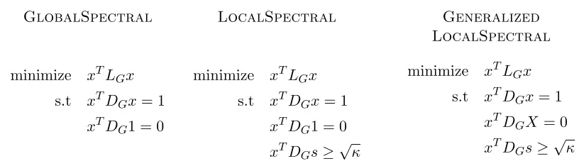
Recall the optimization perspective on how one computes the leading nontrivial global eigenvectors of the normalized Laplacian _LG or, equivalently, of the leading nontrivial gen-eralized eigenvectors ofLG. The first nontrivial eigenvectorv2is the solution to the problem GlobalSpectralthat is presented on the left of Figure 1. Equivalently, although Glob-alSpectral is a non-convex optimization problem, strong duality holds for it and it’s solution may be computed as v2, the leading nontrivial generalized eigenvector of LG. (In this case, the value of the objective isλ2, and global spectral partitioning involves then doing a “sweep cut” over this vector and appealing to Cheeger’s inequality.) The next eigenvector

v3 is the solution toGlobalSpectral, augmented with the constraint thatxTDGv2 = 0; and in general the tth _{generalized eigenvector of}_L

G is the solution to GlobalSpectral, augmented with the constraints that xT_D

Gvi = 0, for i ∈ {2, . . . , t−1}. Clearly, this set of constraints and the constraint xT_D

G1 = 0 can be written as xTDGX = 0, where 0 is a (t−1)-dimensional all-zeros vector, and where X is ann×(t−1) orthogonal matrix whose

ith _{column equals} _v

i (where v1= 1, the all-ones vector, is the first column of X).

Also presented in Figure 1 is LocalSpectral, which includes a constraint that the solution be well-correlated with an input seed set. This LocalSpectral optimization problem was introduced in Mahoney et al. (2012), where it was shown that the solution to LocalSpectralmay be interpreted as a locally-biased version of the second eigenvector of the Laplacian.1 In particular, althoughLocalSpectralis not convex, it’s solution can be computed efficiently as the solution to a set of linear equations that generalize the popular

1. In Mahoney et al. (2012), the locality constraint was actually a quadratic constraint, and thus a somewhat involved analysis was required. In retrospect, given the form of the solution, and in light of the discussion below, it is clear that the quadratic part was not “real,” and thus we present this simpler form of

LocalSpectral here. This should make the connections with our Generalized LocalSpectral

(7)

GlobalSpectral

minimize xTLGx

s.t xTDGx= 1

xTDG1 = 0

LocalSpectral

minimize xTLGx

s.t xTDGx= 1

xTDG1 = 0

xTDGs≥√κ

Generalized LocalSpectral

minimize xT_L Gx s.t xT_D

Gx= 1

xT_D

GX= 0

xT_D

Gs≥

√ κ

Figure 1: Left: The usualGlobalSpectralpartitioning optimization problem; the vector achieving the optimal solution isv2, the leading nontrivial generalized eigenvector ofLG with respect toDG. Middle: TheLocalSpectraloptimization problem, which was originally introduced in Mahoney et al. (2012); for κ = 0, this co-incides with the usual global spectral objective, while for κ > 0, this produces solutions that are biased toward the seed vectors. Right: TheGeneralized Lo-calSpectraloptimization problem we introduce that includes both the locality constraint and a more general orthogonality constraint. Our main algorithm for computing semi-supervised eigenvectors will iteratively compute the solution to Generalized LocalSpectralfor a sequence ofXmatrices. In all three cases, the optimization variable isx_∈Rn.

Personalized PageRank procedure; in addition, by performing a sweep cut and appealing to a variant of Cheeger’s inequality, this locally-biased eigenvector can be used to perform locally-biased spectral graph partitioning (Mahoney et al., 2012).

3.2 Our Main Algorithm

We will formulate the problem of computing semi-supervised vectors in terms of a primitive optimization problem of independent interest. Consider the Generalized LocalSpec-tral optimization problem, as shown in Figure 1. For this problem, we are given a graph

G = (V, E), with associated Laplacian matrix LG and diagonal degree matrix DG; an in-dicator vector s of a small “seed set” of nodes; a correlation parameter κ _∈[0,1]; and an

n_×ν constraint matrix X that may be assumed to be an orthogonal matrix. We will as-sume (without loss of generality) that sis properly normalized and orthogonalized so that

sT_D

Gs= 1 and sTDG1 = 0. While scan be a general unit vector orthogonal to 1, it may be helpful to think ofsas the indicator vector of one or more vertices inV, corresponding to the target region of the graph.

In words, the problemGeneralized LocalSpectralasks us to find a vectorx∈Rn that minimizes the variance xT_L

(8)

n-dimensional all-ones vector, which is the trivial eigenvector LG, in which case X is an

n×1 matrix; and to compute each subsequent semi-supervised eigenvector, we let the columns of X consist of 1 and the other semi-supervised eigenvectors found in each of the previous iterations.

To show that Generalized LocalSpectral is efficiently-solvable, note that it is a quadratic program with only one quadratic constraint and one linear equality constraint.2 In order to remove the equality constraint, which will simplify the problem, let’s change variables by defining the n_×(n₋ν) matrixF as

{x:XTDGx= 0}={x:x=Fxˆ}.

That is, F is a span for the null space of XT_{; and we will take} _F _{to be an orthogonal} matrix. In particular, this implies thatFT_F _{is an (}_n₋_ν₎_×₍_n₋_ν_{) Identity and}_{F F}T _{is an}

n_×n Projection. Then, with respect to the ˆx variable, Generalized LocalSpectral becomes

minimize

y xˆ

T_FT_L GF y

subject to ˆxT_FT_D

GFxˆ= 1, ˆ

xT_FT_D

Gs≥

√ κ.

(1)

In terms of the variablex, the solution to this optimization problem is of the form

x∗ = cF FT ₍_L

G−γDG)F

+

FT_D

Gs

= c F FT (LG−γDG)F FT

+

DGs, (2)

for a normalization constant c _∈(0,_∞) and for some γ that depends on √κ. The second line follows from the first since F is an n×(n−ν) orthogonal matrix. This so-called “S-procedure” is described in greater detail in Chapter 5 and Appendix B of (Boyd and Vandenberghe, 2004). The significance of this is that, although it is a non-convex opti-mization problem, the Generalized LocalSpectral problem can be solved by solving a linear equation, in the form given in Eqn. (2).

Returning to our problem of computing semi-supervised eigenvectors, recall that, in addition to the input for theGeneralized LocalSpectralproblem, we need to specify a positive integer k that indicates the number of vectors to be computed. In the simplest case, we would assume that we would like the correlation to be “evenly distributed” across allkvectors, in which case we will require that each vector ispκ/k-well-correlated with the input seed set vectors; but this assumption can easily be relaxed, and thus Algorithm 1 is formulated more generally as taking ak-dimensional vectorκ= [κ1, . . . , κk]T of correlation coefficients as input.

To compute the first semi-supervised eigenvector, we will letX= 1, the all-ones vector, in which case the first nontrivial semi-supervised eigenvector is

x∗₁ =c(LG−γ1DG)+DGs, (3)

(9)

whereγ1is chosen to saturate the part of the correlation constraint along the first direction. (Note that the projections F FT _{from Eqn. 2 are not present in Eqn. 3 since by design}

sT_D

G1 = 0.) That is, to find the correct setting of γ1, it suffices to perform a binary search over the possible values of γ1 in the interval (−vol(G), λ2(G)) until the correlation constraint is satisfied, that is, until (sT_D

Gx1)2 is sufficiently close to κ1.

To compute subsequent semi-supervised eigenvectors, i.e., at steps t = 2, . . . , k if one ultimately wants a total of k semi-supervised eigenvectors, then one lets X be the n_×t

matrix of the form

X = [1, x∗₁, . . . , x∗_t₋₁], (4)

where x∗₁, . . . , x∗_t₋₁ are successive semi-supervised eigenvectors; and the projection matrix

F FT _{is of the form}

F FT =I−DGX(XTDGDGX)−1XTDG,

due to the the degree-weighted inner norm.

Then, by Eqn. (2), the tth _{semi-supervised eigenvector takes the form}

x∗_t = c F FT₍_L

G−γtDG)F FT

+

DGs.

Algorithm 1 Main algorithm to compute semi-supervised eigenvectors Require: LG, DG, s, κ= [κ1, . . . , κk]T, such thatsTDG1 = 0,sTDGs= 1,κT1≤1

1: X= [1]

2: fort= 1 tokdo

3: F FT_←_I₋_D

GX(XTDGDGX)−1XTDG

4: > ←λ2whereF FTLGF FTv2=λ2F FTDGF FTv2

5: ⊥ ← −vol(G) 6: repeat

7: γt←(⊥+>)/2 (Binary search overγt)

8: xt←(F FT(LG−γtDG)F FT)+F FTDGs

9: Normalizextsuch thatxTtDGxt= 1

10: if(xT

tDGs)2> κtthen⊥ ←γtelse> ←γtend if

11: untilk(xT

tDGs)2−κtk ≤ork(⊥+>)/2−γtk ≤

12: AugmentX withx∗t by lettingX= [X, x∗t].

13: end for

In more detail, Algorithm 1 presents pseudo-code for our main algorithm for computing semi-supervised eigenvectors. The algorithm takes as input a graph G = (V, E), a seed set s (which could be a general vector s_∈Rn, subject for simplicity to the normalization constraintssT_D

G1 = 0 andsTDGs= 1, but which is most easily thought of as an indicator vector for the local “seed set” of nodes), a number k of vectors we want to compute, and a vector of locality parameters (κ1, . . . , κk), where κi ∈ [0,1] and Pk_i=1κi = 1 (where, in the simplest case, one could chooseκi=κ/k,∀i, for someκ∈[0,1]). Several things should be noted about our implementation of our main algorithm. First, as we will discuss in more detail below, we compute the projection matrixF FT _only_implicitly_{. Second, a na¨ıve} approach to Eqn. (2) does not immediately lead to an efficient solution, since DGswill not be in the span of (F FT₍_L

G−γDG)F FT), thus leading to a large residual. By changing variables so thatx=F FT_y_{, the solution becomes}

(10)

Since F FT _{is a projection matrix, this expression is equivalent to}

x∗_t ∝ F FT(LG−γtDG)F FT

+

F FTDGs. (5)

Third, regarding the solutionxi, we exploit thatF FT(LG−γiDG)F FT is an SPSD matrix, and we apply the conjugate gradient method, rather than computing the explicit pseudoin-verse. That is, in the implementation we never explicitly represent the dense matrixF FT_, but instead we treat it as an operator and we simply evaluate the result of applying a vector to it on either side. Fourth, we use that λ2 can never decrease (here we refer toλ2 as the smallest non-zero eigenvalue of the modified matrix), so we only recalculate the upper bound for the binary search when an iteration saturates without satisfying _k(xT

tDGs)2−κtk ≤. Estimating the bound is critical for the semi-supervised eigenvectors to be able to inter-polate all the way to the global eigenvectors of the graph, so in Section 3.4 we return to a discussion on efficient strategies for computing the leading nontrivial eigenvalue of LG projected down onto the space perpendicular to the previously computed solutions.

From this discussion, it should be clear that Algorithm 1 solves the semi-supervised eigenvector problem by solving in an iterative manner optimization problems of the form of Generalized LocalSpectral; and that the running time of Algorithm 1 boils down to solving a sequence of linear equations.

3.3 Discussion of Our Main Algorithm

There is a natural “regularization” interpretation underlying our construction of semi-supervised eigenvectors. To see this, recall that the first step of our algorithm can be computed as the solution of a set of linear equations

x∗ =c(LG−γDG)+DGs, (6)

for some normalization constant c and someγ that can be determined by a binary search over (₋vol(G), λ2(G)); and that subsequent steps compute the analogous quantity, sub-ject to additional constraints that the solution be orthogonal to the previously-computed vectors. The quantity (LG−γDG)+ can be interpreted as a “regularized” version of the pseudoinverse of L, where γ _∈ (_−∞, λ2(G)) serves as the regularization parameter. This interpretation has recently been made precise: Mahoney and Orecchia (2011) show that running a PageRank computation—as well as running other diffusion-based procedures— exactly optimizes a regularized version of the GlobalSpectral (or LocalSpectral, depending on the input seed vector) problem; and (Perry and Mahoney, 2011) provide a precise statistical framework justifying this.

The usual interpretation of PageRank involves “random walkers” who uniformly (or non-uniformly, in the case of Personalized PageRank) “teleport” with a probability α _∈

(0,1). As described in (Mahoney et al., 2012), choosingα∈(0,1) corresponds to choosing

γ _∈(_−∞,0). By rearranging Eqn. (6) as

x∗ = c((DG−AG)−γDG)+DGs

= c

1₋γ

DG−

1 1₋γAG

+

DGs

= c

1₋γD −1 G

I− 1

1₋γAGD −1 G

+

(11)

we recognize AGD_G−1 as the standard random walk matrix, and it becomes immediate that the solution based on random walkers,

x∗= c

1−γD −1

G I+

∞ X

i=1

1 1−γD

−1 G AG

i!

DGs,

is divergent for γ > 0. Since γ = λ2(G) corresponds to no regularization and γ → −∞ corresponds to heavy regularization, viewing this problem in terms of solving a linear equa-tion is formally more powerful than viewing it in terms of random walkers. That is, while all possible values of the regularization parameter—and in particular the (positive) value

λ2(·)—are achievable algorithmically by solving a linear equation, only values in (−∞,0) are achievable by running a PageRank diffusion. In particular, if the optimal value of γ

that saturates theκ-dependent locality constraint is negative, then running the PageRank diffusion could find it; otherwise, the “best” one could do will still not saturate the locality constraint, in which case some of the intended correlation is “unused.”

An important technical and practical point has to do with the precise manner in which the ith _{vector is well-correlated with the seed set} _s_{. In our formulation, this is captured} by alocality parameter γi that is chosen (via a binary search) to “saturate” the correlation condition, i.e., so that the ith _{vector is} _κ/k_{-well-correlated with the input seed set. As a} general rule, successiveγis need to be chosen that successive vectors are less well-localized around the input seed set. (Alternatively, depending on the application, one could choose this parameter so that successive γis are equal; but this will involve “sacrificing” some amount of the κ/k correlation, which will lead to the last or last few eigenvectors being very poorly-correlated with the input seed set. These tradeoffs will be described in more detail below.) Informally, if s is a seed set consisting of a small number of nodes that are “nearby” each other, then to maintain a given amount of correlation, we must “view” the graph over larger and larger size scales as we compute more and more semi-supervised eigenvectors. More formally, we need to let the value of the regularization parameter γ at theith _{round, we call it}_γ

i, vary for eachi∈ {1, . . . , k}. That is,γi is not pre-specified, but it is chosen via a binary search over the region (₋vol(G), λ2(·)), whereλ2(·) is the leading nontrivial eigenvalue ofLG projected down onto the space perpendicular to the previously-computed vectors (which is in general larger thanλ2(G)). In this sense, our semi-supervised eigenvectors are both “locally-biased”, in a manner that depends on the input seed vector and correlation parameter, and “regularized”, in a manner that depends on the local graph structure.

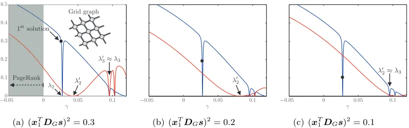
To illustrate the previous discussion, Figure 2 considers the two-dimensional grid. In each subfigure, the blue curve shows the correlation with a single seed node as a function of γ for the leading semi-supervised eigenvector, and the black dot illustrates the value of

γ for three different values of the locality parameterκ. This relationship between κ and γ

is in general non-convex, but it is monotonic for γ _∈ (₋vol(G), λ2(G)). The red curve in each subfigure shows the decay for the second semi-supervised eigenvector. Recall that it is perpendicular to the first semi-supervised eigenvector, that the decay is monotonic for

(12)

κ

γ

−00.05 0 0.05 0.1

0.1 0.2 0.3 0.4 0.5

Grid graph

λ2 λ

′

2

1st_solution

PageRank

3λ′3≈λ3

(a) (xT1DGs)2= 0.3

γ

−0.05 0 0.05 0.1

λ′2

(b) (xT1DGs)2= 0.2

γ

−0.05 0 0.05 0.1

λ′ 2≈λ3

(c) (xT1DGs)2= 0.1

Figure 2: Interplay between the γ parameter and the correlationκ that a semi-supervised eigenvector has with a seed s on a two-dimensional grid. In Figure 2(a)-2(c), we vary the locality parameter for the leading semi-supervised eigenvector, which in each case leads to a value of γ which is marked by the black dot on the blue curve. This allows us to illustrate the influence on the relationship betweenγ and

κ on the next semi-supervised eigenvector. Figure 2(a) also highlights the range

(γ <0) in which Personalized PageRank can be used for computing solutions to

semi-supervised eigenvectors.

parameter that leads to a value of γ that is closer to λ2, thereby increasing the value of

λ0₂. Finally, in Figure 2(c), the locality parameter is such that the leading semi-supervised eigenvector almost coincides with v2; this results in λ02 ≈ λ3, as required if we were to compute the global eigenvectors.

3.4 Bounding the Binary Search

For the following derivations it is more convenient to consider the normalized graph Lapla-cian, in which case we define the first solution as

y1=c(LG−γ1I)+D1/2_G s, (7)

where x∗₁ =D−_G1/2y1. This approach is convenient since the projection operator with null space defined by previous solutions can be expressed as F FT ₌_I ₋_{Y Y}T_{, assuming that}

YT_Y _{= 1. That is,}_Y _{is of the form}

Y = [D_G1/2, y₁∗, . . . , y_t∗₋₁],

wherey∗_i are successive solutions to Eqn. (7). In the following the type of projection opera-tor will be implicit from the context, i.e., when working with the combinaopera-torial graph Lapla-cianF FT ₌_I₋_D

GX(XTDGDGX)−1XTDG, whereas for the normalized graph Laplacian

F FT ₌_I₋_{Y Y}T_.

(13)

correlation with the seedxT_D

Gs, that can be deduced from the KKT-conditions (Mahoney et al., 2012). Note, that if the upper bound for the binary search > = λ2(F FTLGF FT) is not determined with sufficient precision, the search will (if we underestimate _>) fail to satisfy the constraint, or (if we overestimate _>) fail to converge because the monotonic relationship no longer hold.

By Lemma 1 in Appendix A it follows that λ2(F FTLGF FT) =λ2(LG+ωY YT) when

ω_{→ ∞}. Since the latter term is a sum of two PSD matrices, the value of the upper bound can only increase as stated by Lemma 2 in Appendix A. This is an important property, because if we do not recalculate_>, the previous value is guaranteed to be an underestimate, meaning that the objective will remain convex. Thus, it may be more efficient to first recompute> when the binary search fails to satisfy (xT_D

Gs)2 =κ, meaning that > must be recomputed to increase the search range.

We compute the value for the upper bound of the binary search by transforming the problem in such a way that we can determine the greatest eigenvalue of a new system (fast and robust), and from that, deduce the new value of _>=λ2(F FTLGF FT). We do so by expanding the expression as

F FT_L

GF FT =F FT

I₋D−_G1/2AGD−_G1/2

F FT

=F FT −F FTD_G−1/2AGD_G−1/2F FT =I₋F FT_D−1/2

G AGD

−1/2 G F F

T ₊_{Y Y}T_.

Since all columns of Y will be eigenvectors of F FT_L

GF FT with zero eigenvalue, these will all be eigenvectors of F FT_D−1/2

G AGD

−1/2

G F FT +Y YT with eigenvalue 1. Hence, the largest algebraic eigenvalue λLA(F FTD−G1/2AGD

−1/2

G F FT) can be used to compute the upper bound for the binary search as

>=λ2(F FTLGF FT) = 1−λLA(F FTDG−1/2AGD

−1/2 G F F

T₎_. ₍₈₎

The reason for not considering the largest magnitude eigenvalue, is that AG may be in-definite. Finally, with respect to our implementation we emphasize that F FT _{is used as a} projection operator, and not represented explicitly.

4. Extension of Our Main Algorithm And Implementation Details

(14)

4.1 A Nystr¨om-Based Low-rank Approach

Here we describe the use of the recently-popular Nystr¨om method to speed up the compu-tation of semi-supervised eigenvectors. We do so by considering how a low-rank decompo-sition can be exploited to yield solutions to the Generalized LocalSpectralobjective in Figure 1, where the running time largely depends on a matrix-vector product. These methods are most appropriate when the kernel matrix is reasonably well-approximated by a low-rank matrix (Drineas and Mahoney, 2005; Gittens and Mahoney, 2012; Williams and Seeger, 2000).

Given some low-rank approximation LG ≈I−VΛVT, we apply the Woodbury matrix identity, and we derive an explicit solution for the leading semi-supervised eigenvector

y1 ≈c (1−γ)I −VΛVT

+

D1/2_G s

≈c 1

1−γI+

1 (1−γ)2V

Λ−1− 1

1−γI −1

VT

!

D_G1/2s

≈ ₁ c

−γ I+VΣV

T

D1/2_G s,

where Σii= 1−γ1

λi −1

. In order to compute efficiently the subsequent semi-supervised

eigen-vectors we must accommodate for the projection operator F FT ₌ _I ₋_{Y Y}T_{, while yet} exploiting the explicit closed-form inverse (_LG−γI)+ ≈ ₁₋1_γ I+VΣVT

. However, the projection operator complicates the expression, since the previous solution can be spanned by multiple global eigenvectors, so leveraging from the low-rank decomposition is more difficult for the inverse (F FT₍_L

G−γI)F FT)+.

Conveniently, we can decouple the projection operator by treating the orthogonality constraint using a Lagrangian approach, such that the solution can be expressed as

yt=c LG−γI+ωY YT

+

D1/2_G s,

where ω ≥ 0 denotes the associated Lagrange multiplier, and where the sign is deduced from the KKT conditions. Applying the Woodbury matrix identity is now straightforward

Pγ+ωY YT

+

=Pγ+−ωPγ+Y I+ωYTPγ+Y

+

YTPγ+,

where for notational convenience we have introduced Pγ = LG−γI. By decomposing

YT_P

γ+Y with an eigendecompositionU SUT the equation simplifies as follows

Pγ+ωY YT

+

=Pγ+−ωPγ+Y I+ωU SUT

+

YTPγ+

=Pγ+−Pγ+Y UΩUTYTPγ+, where Ωii= 1 1

ω+Sii

. Note how this result gives a well defined way of controlling the amount of “orthogonality”, and by Lemma 1 in Appendix A, we get exact orthogonality in the limit of ω→ ∞, in which case the expression simplifies to

Pγ+ωY YT

+

(15)

Using the explicit expression forPγ+, the solution now only involves matrix-vector products and the inverse of a small matrix

yt=c Pγ+−Pγ+Y(YTPγ+Y)+YTPγ+

D1/2_G s. (9)

To conclude this section, let us also consider how we can optimize the efficiency of the cal-culation ofλ2(F FTLGF FT) used for bounding the binary search in Algorithm 1. According to Eqn. (8) the bound can be calculated efficiently as_>= 1₋λLA(F FTD_G−1/2AGD_G−1/2F FT). However, by substituting withD−_G1/2AGD_G−1/2≈VΛVT, we can exploit low-rankness since

>= 1−λLA(F FTVΛVTF FT) = 1−λLA(Λ1/2VTF FTVΛ1/2), where the latter is a much smaller system.

4.2 A Push-Peeling Heuristic

Here we present a variant of our main algorithm that exploits the connections between diffusion-based procedures and eigenvectors, allowing semi-supervised eigenvectors to be efficiently computed for large networks. This is most well-known for the leading nontrivial eigenvectors of the graph Laplacian (Chung, 1997); but recent work has exploited these connections in the context of performing locally-biased spectral graph partitioning (Spiel-man and Teng, 2004; Andersen et al., 2006; Mahoney et al., 2012). In particular, we can compute the locally-biased vector using the first step of Algorithm 1, or alternatively we can compute it using a locally-biased random walk of the form used in (Spielman and Teng, 2004; Andersen et al., 2006). Here we present a heuristic that works by peeling off com-ponents from a solution to the PageRank problem, and by exploiting the regularization interpretation of γ, we can from these components obtain the subsequent semi-supervised eigenvectors.

Specifically, we focus on the Push algorithm by Andersen et al. (2006). This algorithm approximates the solution to PageRank very efficiently, by exploiting the local modifications that occur when the seed is highly concentrated. This makes our algorithm very scalable and applicable for large-scale data, since only the local neighborhood near the seed set will be touched by the algorithm. In comparison, by solving the linear system of equations we explicitly touch all nodes in the graph, even though most spectral rankings will be below the computational precision (Boldi and Vigna, 2011).

We adapt a similar notation as in Andersen et al. (2006) and start by defining the usual PageRank vector pr(α, spr) as the unique solution of the linear system

pr(α, spr) =αspr+ (1−α)AGDG−1pr(α, spr), (10) whereαis the teleportation parameter, andspris the sparse starting vector. For comparison, the push algorithm by Andersen et al. (2006) computes an approximate PageRank vector pr(α0, spr) for a slightly different system

pr(α0, spr) =α0spr+ (1−α0)Wpr(α0, spr),

(16)

of the respective teleportation parameter. Thus, it is straightforward to verify that these teleportation parameters and the γ parameter of Eqn. (6) are related as

α= 2α0

1 +α0 ⇔α0 = α

2₋α ⇔α

0₌ γ

γ₋2,

and that the leading semi-supervised eigenvector for γ_∈(_−∞,0) can be approximated as

x∗₁ _≈ c

−γD

−1 G pr

γ

γ−2, DGs

.

To generalize subsequent semi-supervised eigenvectors to this diffusion based framework, we need to accommodate for the projection operator such that subsequent solutions can be expressed in terms of graph diffusions. By requiring distinct values of γ for all semi-supervised eigenvectors, we may use the solution for the leading semi-semi-supervised eigenvector and then systematically “peel off” components, thereby obtaining the solution of one of the consecutive semi-supervised eigenvectors. By Lemma 5, in Appendix A the general solution in Eqn. (5) can be approximated by

x∗_t _≈c I₋XXTDG

(LG−γtDG)+DGs, (11) under the assumption that all γk for 1 < k ≤ t are sufficiently apart. If we think about

γk as being distinct eigenvalues of the generalized eigenvalue problem LGxk = γkDGxk, then it is clear that Eqn. (11), correctly computes the sequence of generalized eigenvectors. This is explained by the fact that (LG−γtDG)+DGs can be interpreted as the first step of the Rayleigh quotient iteration, where γt is the estimate of the eigenvalue, and DGs is the estimate of the eigenvector. Given that the estimate of the eigenvalue is right, this algorithm will in the initial step compute the corresponding eigenvector, and the operator

I −XXT_D

G

will be superfluous, as the global eigenvectors are already orthogonal in the degree-weighted norm. To quantify the failure modes of the approximation, let us consider what happens when γ2 starts to approach γ1. What constitutes the second solution for a particular value of γ2 is the perpendicular component with respect to the projection onto the solution given by γ1. As γ2 approaches γ1, this perpendicular part diminishes and the solution becomes ill-posed. Fortunately, we can easily detect such issues during the binary search in Algorithm 1, and in general the approximation has turned out to work very well in practice as our experimental results in Section 5 show.

In terms of the approximate PageRank vector pr(α0, spr) , the general approximate solution takes the following form

D−_G1pr

γt

γt−2

, DGs

. (12)

(17)

Lemma 3 in Appendix A, because the leading ones will then span the entire space of the seed set. As the choice of is important for the applicability of our algorithm, we will in Section 5 investigate the influence of this parameter on large data graphs.

To conclude this section, we consider an important implementation detail that have been omitted so far. In the work of Mahoney et al. (2012) the seed vector was defined to be perpendicular to the all-ones vector, and for the sake of consistency we have chosen to define it in the same way. The impact of projecting the seed set to a space that is perpendicular to the all-ones vector is that the resulting seed vector is no longer sparse, making the use of the Push algorithm in Eqn. (12) inefficient. The seed vector can, however, without loss of generality, be defined as s _∝ D_G−1/2 I₋v0v0T

s0 where s0 is the sparse seed, and v0 ∝ diag

D1/2_G is the leading eigenvector of the normalized graph Laplacian (corresponding to the all-ones vector of the combinatorial graph Laplacian). If we substitute with this expression for the seed in Eqn. (12), it follows by plain algebra (see Appendix B) that

D−_G1pr

γt

γt−2

, D1/2_G s0

−D_G−1/2v0v0Ts0

. (13)

Now the Push algorithm is only defined on the sparse seed set making the the expression very scalable. Finally, the Push algorithm maintains a queue of high residual nodes that are yet to be processed. The order in which nodes are processed influences the overall running time, and in Boldi and Vigna (2011) preliminary experiments showed that a FIFO queue resulted in the best performance for large values of γ, as compared to a priority queue that scales logarithmically. For this reason we have chosen to use a FIFO queue in our implementation.

5. Empirical Results

In this section, we provide a detailed empirical evaluation of the method of semi-supervised eigenvectors and how it can be used for locally-biased machine learning. Our goal is two-fold: first, to illustrate how the “knobs” of the method work; and second, to illustrate the usefulness of the method in real applications. To do this, we consider several classes of data.

• Toy data. In Section 5.1, we consider one-dimensional examples of the popular “small world” model (Watts and Strogatz, 1998). This is a parameterized family of models that interpolates between low-dimensional grids and random graphs; and, as such, it allows us to illustrate the behavior of the method and its various parameters in a controlled setting.

• Congressional voting data. In Section 5.2, we consider roll call voting data from the United States Congress that are based on (Poole and Rosenthal, 1991). This is an example of realistic data set that has relatively-simple global structure but nontrivial local structure that varies with time (Cucuringu and Mahoney, 2011); and thus it allows us to illustrate the method in a realistic but relatively-clean setting.

(18)

data allow us to illustrate how the method may be used to perform locally-biased versions of common machine learning tasks such as smoothing, clustering, and kernel construction.

• Large-scale network data. In Section 5.4, we consider large-scale network data, and demonstrate significant performance improvements of the push-peeling heuris-tic compared to solving the same equations using a conjugate gradient solver. These improvements are demonstrated on data sets from the DIMACS implementation chal-lenge, as well as on large web-crawls with more then 3 billion non-zeros in the adja-cency matrix (Paolo et al., 2004, 2011; Paolo and Sebastiano, 2004).

5.1 Small-World Data

The first data sets we consider are networks constructed from the so-called small-world model. This model can be used to demonstrate how semi-supervised eigenvectors focus on specific target regions of a large data graph to capture slowest modes of local variation; and it can also be used to illustrate how the “knobs” of the method work, e.g., how κ and γ

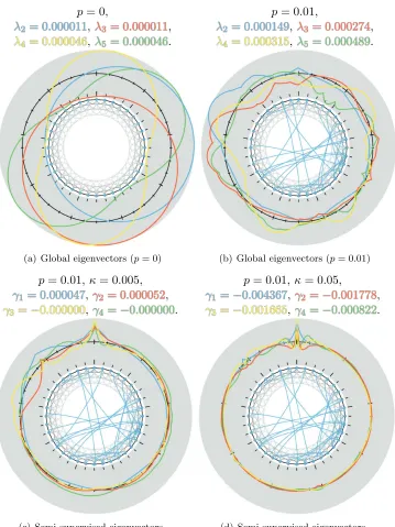
interplay, in a practical setting. In Figure 3, we plot the usual global eigenvectors, as well as locally-biased semi-supervised eigenvectors, around illustrations of non-rewired and rewired realizations of the small-world graph, i.e., for different values of the rewiring probability p

and for different values of the locality parameterκ.

To start, in Figure 3(a) that we show a graph with no randomly-rewired edges (p= 0) and a parameterκ such that the global eigenvectors are obtained. This yields a symmetric graph with eigenvectors corresponding to orthogonal sinusoids, i.e., the first two capture the slowest mode of variation and correspond to a sine and cosine with equal random phase-shift (up to a rotational ambiguity). In Figure 3(b), random edges have been added with probabilityp= 0.01 and the parameter κis still chosen such that the global eigenvectors— now of the rewired graph—are obtained. Note the many small kinks in the eigenvectors at the location of the randomly added edges. Note also the slow mode of variation in the interval on the top left; a normalized-cut based on the leading global eigenvector would extract this region, since the remainder of the ring is more well-connected due to the random rewiring.

(19)

p= 0,

λ2 = 0.000011

λ2= 0.000011

λ2 = 0.000011

λ2= 0.000011

λ2 = 0.000011

λλ22 = 0= 0..000011000011,λ3λλλλλλ3λ3λ3λλλλλλλλ3333333333333= 0= 0= 0= 0= 0= 0= 0= 0= 0= 0= 0= 0= 0= 0= 0= 0= 0...000011000011000011000011000011000011000011000011000011000011000011000011000011000011000011000011000011,

λ4 = 0.000046

λ4= 0.000046

λ4 = 0.000046

λ4= 0.000046

λ4 = 0.000046

λλ44 = 0= 0..000046000046,λλ5λλλλλλλλ5λλλλλλλ555555555555555= 0= 0= 0= 0= 0= 0= 0= 0= 0= 0= 0= 0= 0= 0= 0= 0= 0...000046000046000046000046000046000046000046000046000046000046000046000046000046000046000046000046000046.

(a) Global eigenvectors (p= 0)

p= 0.01,

λ2= 0.000149

λλλ2λ2λλ2222 = 0= 0= 0= 0= 0= 0...000149000149000149000149000149000149

λ2 = 0.000149

λ2= 0.000149

λ2 = 0.000149

λ2= 0.000149

λ2= 0.000149,λ3λλ3λλλλλλλλ3λ3λλλλλ3333333333333= 0= 0= 0= 0= 0= 0= 0= 0= 0= 0= 0= 0= 0= 0= 0= 0= 0...000274000274000274000274000274000274000274000274000274000274000274000274000274000274000274000274000274,

λ4= 0.000315

λλλλλ4λ44444 = 0= 0= 0= 0= 0= 0...000315000315000315000315000315000315

λ4 = 0.000315

λ4= 0.000315

λ4 = 0.000315

λ4= 0.000315

λ4= 0.000315,λλλλλ5λλλλλλλλ5λλλλ555555555555555= 0= 0= 0= 0= 0= 0= 0= 0= 0= 0= 0= 0= 0= 0= 0= 0= 0...000489000489000489000489000489000489000489000489000489000489000489000489000489000489000489000489000489.

(b) Global eigenvectors (p= 0.01)

p= 0.01, κ= 0.005,

γ1 = 0.000047 γ1= 0.000047 γ1= 0.000047 γγ11 = 0= 0..000047000047

γ1 = 0.000047

γ1= 0.000047

γ1= 0.000047 γ1 = 0.000047 γ1 = 0.000047

γ1 = 0.000047

γ1 = 0.000047 γ1 = 0.000047 γ1 = 0.000047 γ1 = 0.000047

γ1 = 0.000047,γγγγγγγ2γ2γγγγγγ2γγ2γ2222222222222= 0= 0= 0= 0= 0= 0= 0= 0= 0= 0= 0= 0= 0= 0= 0= 0= 0...000052000052000052000052000052000052000052000052000052000052000052000052000052000052000052000052000052,

γ3=−0.000000

γγγγ3γγ33333 ======−−−−−−000000...000000000000000000000000000000000000

γ3 =−0.000000

γ3=−0.000000

γ3 =−0.000000

γ3=−0.000000

γ3=−0.000000,γγγγγ4γγγγγγγγγ4γγγ444444444444444=================−−−−−−−−−−−−−−−−−00000000000000000...000000000000000000000000000000000000000000000000000000000000000000000000000000000000000000000000000000.

(c) Semi-supervised eigenvectors

p= 0.01,κ= 0.05,

γ1 =−0.004367

γ1=−0.004367

γ1 =−0.004367

γ1=−0.004367

γ1 =−0.004367

γγγ111 ===−−−000...004367004367004367,γγγγ2γ2γ2γ2γγγγγγγγγγ2222222222222=================−−−−−−−−−−−−−−−−−00000000000000000...001778001778001778001778001778001778001778001778001778001778001778001778001778001778001778001778001778,

γ3 =−0.001665

γ3=−0.001665

γ3 =−0.001665

γ3=−0.001665

γ3 =−0.001665

γγγ333 ===−−−000...001665001665001665,γγγ4γγγγγγγγγγ4γγγγ444444444444444=================−−−−−−−−−−−−−−−−−00000000000000000...000822000822000822000822000822000822000822000822000822000822000822000822000822000822000822000822000822.

(d) Semi-supervised eigenvectors

(20)

has the effect of decreasing the value ofγt), making the semi-supervised eigenvectors more localized in the neighborhood of the seed. It should be clear that, in addition to being determined by the locality parameter, we can think ofγ as a regularizer biasing the global eigenvectors towards the region near the seed set. That is, variation in eigenvectors that are near the initial seed (in the modified graph topology) are most important, while variation that is far away from the initial seed matters much less.

5.2 Congressional Voting Data

The next data set we consider is a network constructed from a time series of roll call voting patterns from the United States Congress that are based on Poole and Rosenthal (1991). This is a particularly well-structured social network for which there is a great deal of meta-information, and it has been studied recently with graph-based methods (Mucha et al., 2010; Waugh et al., 2009; Cucuringu and Mahoney, 2011). Thus, it permits a good illustration of the method of semi-supervised eigenvectors in a real application (Poole, Fall 2005). This data set is known to have nontrivial time-varying structure at different time steps, and we will illustrate how the method of semi-supervised eigenvectors can perform locally-biased classification with a traditional kernel-based algorithm.

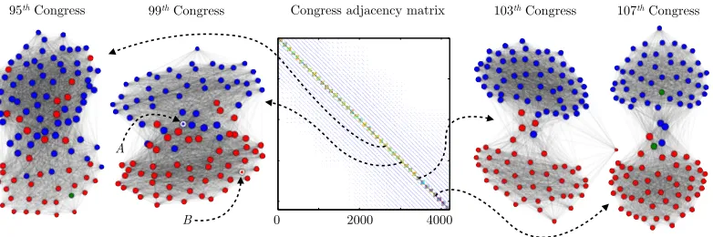
In more detail, we evaluate our method by considering the known Congress data-set containing the roll call voting patterns in the U.S Senate across time. We considered Senates in the 70th _{Congress through the 110}th _{Congress, thus covering the years 1927 to 2008.} During this time, the U.S went from 48 to 50 states, hence the number of senators in each of these 41 Congresses was roughly the same. We constructed anN×N adjacency matrix, with N = 4196 (41 Congresses each with _≈ 100 Senators) where Aij ∈ [0,1] represents the extent of voting agreement between legislatorsiand j, and where identical senators in adjacent Congresses are connected with an inter-Congress connection strength. We then considered the Laplacian matrix of this graph, constructed in the usual way (Cucuringu and Mahoney, 2011).

95th_Congress ₉₉th_Congress _{Congress adjacency matrix} ₁₀₃th_Congress ₁₀₇th_Congress

A

B 0 2000 4000

(21)

Figure 4 visualizes the adjacency matrix, along with four of the individual Congresses, color coded by party. This illustrates that these data should be viewed—informally—as a structure (depending on the specific voting patterns of each Congress) evolving along a one-dimensional temporal axis, confirming the results of Cucuringu and Mahoney (2011). Note that the latter two Congresses are significantly better described by a simple two-clustering than the former two Congresses, and an examination of the two-clustering properties of each of the 40 Congresses reveals significant variation in the local structure of individual Congresses, in a manner broadly consistent with Poole (Fall 2005) and Poole and Rosenthal (1991). In particular, the more recent Congresses are significantly more polarized.

v2

0 2000 4000

x1,κ= 0.001

0 2000 4000

x1,κ= 0.1

0 2000 4000

x1,κ= 0.1

0 2000 4000

v3

0 2000 4000

x2,κ= 0.001

0 2000 4000

x2,κ= 0.1

0 2000 4000

x2,κ= 0.1

0 2000 4000

v4

0 2000 4000

x3,κ= 0.001

0 2000 4000

x3,κ= 0.1

0 2000 4000

x3,κ= 0.1

0 2000 4000

Figure 5: First column: The leading three nontrivial global eigenvectors. Second column: The leading three semi-supervised eigenvectors seeded (circled node) in an artic-ulation point between the two parties in the 99th _{Congress (see Figure 4), for} correlation κ = 0.001. Third column: Same seed as previous column, but for a correlation of κ = 0.1. Notice the localization on the third semi-supervised eigenvector. Fourth column: Same correlation as the previous column, but for another seed node well within the cluster of Republicans. Notice the localization on all three semi-supervised eigenvectors.

(22)

one-dimensional temporal scaffolding. Also shown in the first column are the values of that eigenfunction for the members of the 99th _{Congress, illustrating that there is} _not _{a good} separation based on party affiliations. The next three vertical columns of Figure 5 illus-trate various localized eigenvectors computed by starting with a seed node in the 99th Congress. For the second column, we visualize the semi-supervised eigenvectors for a very low correlation (κ= 0.001), which corresponds to only a weak localization—in this case one sees eigenvectors that look very similar to the global eigenvectors, and the elements of the eigenvector on that Congress do not reveal partitions based on the party cuts.

The third and fourth column of Figure 5 illustrate the semi-supervised eigenvectors for a much higher correlation (κ = 0.1), meaning a much stronger amount of locality. In particular, the third column starts with the seed node marked A in Figure 4, which is at the articulation point between the two parties, while the fourth column starts with the seed node marked B, which is located well within the cluster of Republicans. In both cases the eigenvectors are much more strongly localized on the 99th _{Congress near the seed node,} and in both cases one observes the partition into two parties based on the elements of the localized eigenvectors. Note, however, that when the initial seed is at the articulation point between two parties then the situation is much noisier: in this case, this “partitionability” is seen only on the third semi-supervised eigenvector, while when the initial seed is well within one party then this is seen on all three eigenvectors. Intuitively, when the seed set is strongly within a good cluster, then that cluster tends to be found with semi-supervised eigenvectors (and we will observe this again below). This is consistent with the diffusion interpretation of eigenvectors. This is also consistent with Cucuringu and Mahoney (2011), who observed that the properties of eigenvector localization depended on the local structure of the data around the seed node, as well as the larger scale structure around that local cluster.

Nt h

Congr e s s

C la s s ifi c a t io n a c c u r a c y Global eigenvectors

70 80 90 100 110 0 1 4 1 2 3 4 1

Nt h

Congr e s s

C la s s ifi c a t io n a c c u r a c y

Global eigenvectors, single Congress

70 80 90 100 110

0 1 4 1 2 3 4 1

Nt h

Congr e s s

C la s s ifi c a t io n a c c u r a c y

Semi-sup ervised eigenvectors

70 80 90 100 110

0 1 4 1 2 3 4 1

(23)

To illustrate how these structural properties manifest themselves in a more traditional machine learning task, we also consider the classification task of discriminating between Democrats and Republicans in single Congresses, i.e., we measure to what extent we can ex-tract local discriminative features. To do so, we applyL2-regularizedL2-loss support vector classification with a linear kernel, where features are extracted using the global eigenvec-tors of the entire data set, global eigenveceigenvec-tors from a single Congress (best case measure), and our semi-supervised eigenvectors. Figure 6 illustrates the classification accuracy for 1, 2, and 3 eigenvectors. As reported by Cucuringu and Mahoney (2011), locations that exhibit discriminative information are best found on low-order eigenvectors of this data, explaining why the classifier based global eigenvectors performs poorly. In the classifier based on global eigenvectors in the single Congress we exploita priori knowledge to extract the relevant data, that in a usual situation would be impossible. Hence, this is simply to define a baseline point of reference for the best case classification accuracy. The classifier based on semi-supervised eigenvectors is seeded using a few training samples and performs in-between the two other approaches. Compared to our point of reference, Congresses in the range 88 to 96 do worse with the semi-supervised eigenvectors; whereas for Congresses after 100 the semi-supervised approach almost performs on par, even for a single single eigenvec-tor. This is consistent with the visualization in Figure 4 illustrating that earlier Congresses are less cleanly separable, as well as with empirical evidence indicating heterogeneity due to Southern Democrats in earlier Congresses and the recent increase in party polarization in more recent Congresses, as described in Poole (Fall 2005) and Poole and Rosenthal (1991).

5.3 MNIST Digit Data

The next data set we consider is the well-studied MNIST data set containing 60,000 training digits and 10,000 test digits ranging from 0 to 9; and, with these data, we demonstrate the use of semi-supervised eigenvectors as a feature extraction preprocessing step in a traditional machine learning setting. We construct the full 70,000_×70,000k-NN graph, withk= 10 and with edge weights given by wij = exp(−_σ42

ikxi−xjk

2_{), where} _σ2

i is the Euclidean distance of theith_{node to it’s nearest neighbor; and from this we define the graph Laplacian} in the usual way. We then evaluate the semi-supervised eigenvectors in a transductive learning setting by disregarding the majority of labels in the entire training data. We use a few samples from each class to seed our semi-supervised eigenvectors as well as a few others to train a downstream classification algorithm. For this evaluation, we use the Spectral Graph Transducer (SGT) of Joachims (2003); and we choose to use it for two main reasons. First, the transductive classifier is inherently designed to work on a subset of global eigenvectors of the graph Laplacian, making it ideal for validating that the localized basis constructed by the semi-supervised eigenvectors can be more informative when we are solely interested in the “local heterogeneity” near a seed set. Second, using the SGT based on global eigenvectors is a good point of comparison, because we are only interested in the effect of our subspace representation. (If we used one type of classifier in the local setting, and another in the global, the classification accuracy that we measure would obviously be confounded.) As in Joachims (2003), we normalize the spectrum of both global and semi-supervised eigenvectors by replacing the eigenvalues with some monotonically increasing function. We use λi = i

2

(24)

et al., 2003). Furthermore, we fix the regularization parameter of the SGT to c = 3200, and for simplicity we fixγ = 0 for all semi-supervised eigenvectors, implicitly defining the effective κ = [κ1, . . . , κk]T. Clearly, other correlation distributions κ and other values of

γ parameter may yield subspaces with even better discriminative properties (which is an issue to which we will return in Section 5.3.2 in greater detail).

#Semi-supervised eigenvectors for SGT #Global eigenvectors for SGT

Labeled points 1 2 4 6 8 10 1 5 10 15 20 25

1 : 1 0.39 0.39 0.38 0.38 0.38 0.36 0.50 0.48 0.36 0.27 0.27 0.19 1 : 10 0.30 0.31 0.25 0.23 0.19 0.15 0.49 0.36 0.09 0.08 0.06 0.06 5 : 50 0.12 0.15 0.09 0.08 0.07 0.06 0.49 0.09 0.08 0.07 0.05 0.04 10 : 100 0.09 0.10 0.07 0.06 0.05 0.05 0.49 0.08 0.07 0.06 0.04 0.04 50 : 500 0.03 0.03 0.03 0.03 0.03 0.03 0.49 0.10 0.07 0.06 0.04 0.04 Table 1: Classification error for discriminating between 4s and 9s for the SGT based on,

respectively, semi-supervised eigenvectors and global eigenvectors. The first col-umn from the left encodes the configuration, e.g., 1:10 interprets as 1 seed and 10 training samples from each class (total of 22 samples—for the global approach these are all used for training). When the seed is well-determined and the number of training samples moderate (50:500), then a single semi-supervised eigenvector is sufficient; whereas for less data, we benefit from using multiple semi-supervised eigenvectors. All experiments have been repeated 10 times.

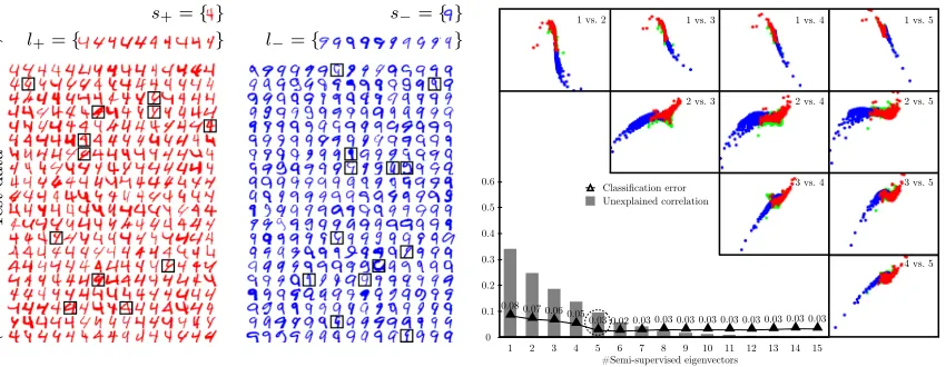
5.3.1 Discriminating Between Pairs of Digits

Here, we consider the task of discriminating between two digits; and, in order to address a particularly challenging task, we work with 4s and 9s. (This is particularly challenging since these two classes tend to overlap more than other combinations since, e.g., a closed 4 can resemble a 9 more than an open 4.) Hence, we expect that the class separation axis will not be evident in the leading global eigenvector, but instead it will be “buried” further down the spectrum; and we hope to find a “locally-biased class separation axis” with locally-biased semi-supervised eigenvectors. Thus, this example will illustrate how semi-supervised eigenvectors can represent relevant heterogeneities in a local subspace of low dimensionality. See Table 1, which summarizes our classification results based on, respectively, semi-supervised eigenvectors and global eigenvectors, when we use the SGT. See also Figure 7 and Figure 8, which illustrate two realizations for the 1:10 configuration. In these two figures, the training samples are fixed; and, to demonstrate the influence of the seed, we have varied the seed nodes. In particular, in Figure 7 the seed nodess+ands−are

located well-within the respective classes; while in Figure 8, they are located much closer to the boundary between the two classes. As intuitively expected, when the seed nodes fall well within the classes to be differentiated, the classification is much better than when the seed nodes are located closer to the boundary between the two classes. See the caption in these figures for further details.

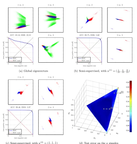
5.3.2 Effect of Choosing The κ Correlation/Locality Parameter

(25)

s+={ }

←

−

−−

T

est

data

−−

−

−→ l+={ }

s−={ }

l−={ }

1 2 3 4 5 6 7 8 9 10 11 12 13 14 15 0.08 0.07 0.06 0.05_{0.03 0.02 0.03 0.03 0.03 0.03 0.03 0.03 0.03 0.03 0.03}

Classification error Unexplained correlation

1 vs. 2 1 vs. 3 1 vs. 4 1 vs. 5

2 vs. 3 2 vs. 4 2 vs. 5

3 vs. 4 3 vs. 5

4 vs. 5

#Semi-supervised eigenvectors 0.6

0.5

0.4

0.3

0.2

0.1

0

Figure 7: Discrimination between 4s and 9s. Left: Shows a subset of the classification re-sults for the SGT based on 5 semi-supervised eigenvectors seeded ins+ and s−,

and trained using samples l+ and l−. Misclassifications are marked with black

frames. Right: Visualizes all test data spanned by the first 5 semi-supervised eigenvectors, by plotting each component as a function of the others. Red (blue) points correspond to 4 (9), whereas green points correspond to remaining digits. As the seed nodes are good representatives, we note that the eigenvectors provide a good class separation. We also plot the error as a function of local dimen-sionality, as well as the unexplained correlation, i.e., initial components explain the majority of the correlation with the seed (effect of γ = 0). The particular realization based on the leading 5 semi-supervised eigenvectors yields an error of

≈0.03 (dashed circle).

For example, will the downstream classifier benefit the most from a uniform distribution or will there exist some other nonuniform distribution that is better? Although this will be highly problem specific, one might hope that in realistic applications the classification performance is not too sensitive to the actual choice of distribution. To investigate the effect in our example of discriminating between 4s and 9s, we consider 3 semi-supervised eigenvectors for various κdistributions. Our results are summarized in Figure 9.