Bayesian Entropy Estimation for Countable Discrete Distributions

Bayesian Entropy Estimation for Countable Discrete

Distributions

Evan Archer∗ [email protected]

Center for Perceptual Systems

The University of Texas at Austin, Austin, TX 78712, USA

Max Planck Institute for Biological Cybernetics Spemannstrasse 41

72076 T¨ubingen, Germany

Il Memming Park∗ [email protected]

Center for Perceptual Systems

The University of Texas at Austin, Austin, TX 78712, USA

Jonathan W. Pillow _{[email protected]}

Department of Psychology, Section of Neurobiology,

Division of Statistics and Scientific Computation, and Center for Perceptual Systems The University of Texas at Austin, Austin, TX 78712, USA

Editor:Lawrence Carin

Abstract

We consider the problem of estimating Shannon’s entropyH from discrete data, in cases where the number of possible symbols is unknown or even countably infinite. The Pitman-Yor process, a generalization of Dirichlet process, provides a tractable prior distribution over the space of countably infinite discrete distributions, and has found major applications in Bayesian non-parametric statistics and machine learning. Here we show that it provides a natural family of priors for Bayesian entropy estimation, due to the fact that moments of the induced posterior distribution overH can be computed analytically. We derive formulas for the posterior mean (Bayes’ least squares estimate) and variance under Dirichlet and Pitman-Yor process priors. Moreover, we show that a fixed Dirichlet or Pitman-Yor process prior implies a narrow prior distribution overH, meaning the prior strongly determines the entropy estimate in the under-sampled regime. We derive a family of continuous measures for mixing Pitman-Yor processes to produce an approximately flat prior over

H. We show that the resulting “Pitman-Yor Mixture” (PYM) entropy estimator is consistent for a large class of distributions. Finally, we explore the theoretical properties of the resulting estimator, and show that it performs well both in simulation and in application to real data.

Keywords: entropy, information theory, Bayesian estimation, Bayesian nonparametrics, Dirichlet process, Pitman–Yor process, neural coding

1. Introduction

Shannon’s discrete entropy appears as an important quantity in many fields, from probability theory to engineering, ecology, and neuroscience. While entropy may be best known for its role in information theory, the practical problem of estimating entropy from samples arises in many applied settings. For example, entropy provides an important tool for quantifying the information carried by neural signals, and there is an extensive literature in neuroscience devoted to estimating the entropy of neural spike trains (Strong et al., 1998; Barbieri et al., 2004; Shlens et al., 2007; Rolls et al., 1999;

Knudson and Pillow, 2013). Entropy is also used for estimating dependency structure and inferring causal relations in statistics and machine learning (Chow and Liu, 1968; Schindler et al., 2007), as well as in molecular biology (Hausser and Strimmer, 2009). Entropy also arises in the study of complexity and dynamics in physics (Letellier, 2006), and as a measure of diversity in ecology (Chao and Shen, 2003) and genetics (Farach et al., 1995).

In these settings, researchers are confronted with data arising from an unknown discrete dis-tribution, and seek to estimate its entropy. One reason for estimating the entropy, as opposed to estimating the full distribution, is that it may be infeasible to collect enough data to estimate the full distribution reliably. The problem is not just that we may not have enough data to estimate the probability of an event accurately. In the so-called “undersampled regime” we may not even observe all events that have non-zero probability. In general, estimating a distribution in this setting is a hopeless endeavor. Estimating the entropy, by contrast, is much easier. In fact, in many cases, entropy can be accurately estimated with fewer samples than the number of distinct

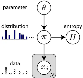
Nonetheless, entropy estimation remains a difficult problem. There is no unbiased estimator for entropy, and the maximum likelihood estimator is severely biased for small data sets (Paninski, 2003). Many previous studies have taken a frequentist approach and focused on methods for computing and reducing this bias (Miller, 1955; Panzeri and Treves, 1996; Strong et al., 1998; Paninski, 2003; Grassberger, 2008). Here, we instead take a Bayesian approach to entropy estimation, building upon an approach introduced by Nemenman and colleagues (Nemenman et al., 2002). Our basic strategy is to place a prior over the space of discrete probability distributions and then perform inference using the induced posterior distribution over entropy. Figure 1 shows a graphical model illustrating the dependencies between the basic quantities of interest.

When there are few samples relative to the total number of symbols, entropy estimation is especially difficult. We refer to this informally as the “under-sampled” regime. In this regime, it is common for many symbols with non-zero probability to remain unobserved, and often we can only bound or estimate thesupport of the distribution (i.e., the number of symbols with non-zero probability). Previous Bayesian approaches to entropy estimation (Nemenman et al., 2002) required

a priori knowledge of the support. Here we overcome this limitation by formulating a prior over the space of countably-infinite discrete distributions. As we will show, the resulting estimator is consistent even when the support of the true distribution is finite.

Our approach relies on Pitman-Yor process (PYP), a two-parameter generalization of the Dirichlet process (DP) (Pitman and Yor, 1997; Ishwaran and James, 2003; Goldwater et al., 2006), which provides a prior distribution over the space of countably infinite discrete distributions. The PYP provides an attractive family of priors in this setting because: (1) the induced posterior distribution over entropy given data has analytically tractable moments; and (2) distributions sampled from a PYP can exhibit power-law tails, a feature commonly observed in data from social, biological and physical systems (Zipf, 1949; Dudok de Wit, 1999; Newman, 2005).

However, we show that a PYP prior with fixed hyperparameters imposes a narrow prior distribution over entropy, leading to severe bias and overly narrow posterior credible intervals given a small data set. Our approach, inspired by Nemenman and colleagues (Nemenman et al., 2002), is to introduce a family of mixing measures over Pitman-Yor processes such that the resulting Pitman-Yor Mixture (PYM) prior provides an approximately non-informative (i.e., flat) prior over entropy.

parameter

distribution

data

entropy

...

Figure 1: Graphical model illustrating the ingredients for Bayesian entropy estimation. Arrows indicate conditional dependencies between variables, and the gray “plate” denotes multiple copies of a random variable (with the number of copiesN indicated at bottom). For entropy estimation, the joint probability distribution over entropyH, datax={xj}, discrete distri-butionπ={πi}, and parameterθ factorizes as: p(H,x,π, θ) =p(H|π)p(x|π)p(π|θ)p(θ). Entropy is a deterministic function ofπ, sop(H|π) =δ(H−P

iπilogπi).The Bayes least squares estimator corresponds to the posterior mean: _E[H|x] =RR

p(H|π)p(π, θ|x)dπdθ.

2. Entropy Estimation

Consider samples x := {xj} N

j=1 drawn iid from an unknown discrete distribution π := {πi} A i=1, p(xj=i) =πi, on a finite or (countably) infinite alphabetXwith cardinalityA. We wish to estimate the entropy ofπ

H(π) =− A X

i=1

πilogπi. (1)

We are interested in the so-called “under-sampled regime,”N A, where many of the symbols remain unobserved. We will see that a naive approach to entropy estimation in this regime results in severely biased estimators and briefly review approaches for correcting this bias. We then consider Bayesian techniques for entropy estimation in general before introducing the Nemenman–Shafee–Bialek (NSB) method upon which the remainder of the article will build.

2.1 Plugin Estimator and Bias-Correction Methods

Perhaps the most straightforward entropy estimation technique is to estimate the distributionπand then use the plugin formula (1) to evaluate its entropy. The empirical distribution ˆπ= (ˆπ1, . . . ,πˆ_A) is computed by normalizing the observed countsn:= (n1, . . . , nA) of each symbol

ˆ

πk=nk/N, nk = N X

i=1

1_{xi=k}, (2)

for eachk∈X. Plugging this estimate forπ into (1), we obtain the so-called “plugin” estimator ˆ

Hplugin=− X

ˆ

πilog ˆπi, (3)

much of which considers the setting in whichAis known and finite. One popular and well-studied method involves taking a series expansion of the bias (Miller, 1955; Treves and Panzeri, 1995; Panzeri and Treves, 1996; Grassberger, 2008) and then subtracting it from the plugin estimate. Other recent proposals include minimizing an upper bound over a class of linear estimators (Paninski, 2003), and a James-Stein estimator (Hausser and Strimmer, 2009). Recently, Wolpert and colleagues have considered entropy estimation in the case of unknown alphabet size (Wolpert and DeDeo, 2013). In that paper, the authors infer entropy under a (finite) Dirichlet prior, but treat the alphabet size itself as a random variable that can be either inferred from the data or integrated out.

Other recent work considers countably infinite alphabets. The coverage-adjusted estimator (CAE) (Chao and Shen, 2003; Vu et al., 2007) addresses bias by combining the Horvitz-Thompson estimator with a nonparametric estimate of the proportion of total probability mass (the “coverage”) accounted for by the observed datax. In a similar spirit, Zhang proposed an estimator based on the Good-Turing estimate of population size (Zhang, 2012).

2.2 Bayesian Entropy Estimation

The Bayesian approach to entropy estimation involves formulating a prior over distributionsπ, and then turning the crank of Bayesian inference to inferH using the posterior distribution. Bayes’ least squares (BLS) estimators take the form

ˆ

H(x) =E[H|x] =

Z

H(π)p(H|π)p(π|x) dπ,

where p(π|x) is the posterior overπ under some prior p(π) and discrete likelihoodp(x|π), and

p(H|π) =δ(H+X i

πilogπi),

sinceH is deterministically related toπ. To the extent thatp(π) expresses our true prior uncertainty over the unknown distribution that generated the data, this estimate is optimal (in a least-squares sense), and the corresponding credible intervals capture our uncertainty aboutH given the data.

For distributions with known finite alphabet sizeA, the Dirichlet distribution provides an obvious choice of prior due to its conjugacy with the categorical distribution. It takes the form

pDir(π)∝ A Y

i=1 πa_i−1,

forπon theA-dimensional simplex (πi≥1, P_{πi = 1), wherea >0 is a “concentration” parameter} (Hutter, 2002). Many previously proposed estimators can be viewed as Bayesian under a Dirichlet

prior with particular fixed choice ofa(Hausser and Strimmer, 2009).

2.3 Nemenman-Shafee-Bialek (NSB) Estimator

In a seminal paper, Nemenman and colleagues showed that for finite distributions with knownA, Dirichlet priors with fixed a impose a narrow prior distribution over entropy (Nemenman et al., 2002). In the under-sampled regime, Bayesian estimates based on such highly informative priors are essentially determined by the value of a. Moreover, they have undesirably narrow posterior credible intervals, reflecting narrow prior uncertainty rather than strong evidence from the data. (These estimators generally give incorrect answers with high confidence!). To address this problem,

Nemenman and colleagues suggested a mixture-of-Dirichlets prior

p(π) = Z

where pDir(π|a) denotes a Dir(a) prior onπ, andp(a) denotes a set of mixing weights, given by p(a)∝ d

daE[H|a] =Aψ1(Aa+ 1)−ψ1(a+ 1), (5) where _E[H|a] denotes the expected value ofH under a Dir(a) prior, andψ1(·) denotes the tri-gamma function. To the extent thatp(H|a) resembles a delta function, (4) and (5) imply a uniform prior for H on [0,logA]. The BLS estimator under the NSB prior can be written

ˆ

Hnsb=E[H|x] =

Z Z

H(π)p(π|x, a)p(a|x) dπda

= Z

E[H|x, a]

p(x|a)p(a) p(x) da,

whereE[H|x, a] is the posterior mean under a Dir(a) prior, andp(x|a) denotes the evidence, which has a P´olya distribution (Minka, 2003)

p(x|a) = Z

p(x|π)p(π|a) dπ

= (N!)Γ(Aa) Γ(a)AΓ(N+Aa)

A Y

i=1

Γ(ni+a) ni! .

The NSB estimate ˆHnsb and its posterior variance are easily computable via 1D numerical integration inausing closed-form expressions for the first two moments of the posterior distribution ofH given a. The forms for these moments are discussed in previous work (Wolpert and Wolf, 1995; Nemenman et al., 2002), but the full formulae have to our knowledge never been explicitly shown. Here we state the results,

E[H|x, a] =ψ0( ˜N+ 1)− X

i ˜ ni

˜

Nψ0(˜ni+ 1) (6)

E[H2|x, a] =

X

i6=k ˜ ni˜nk

( ˜N+ 1) ˜NIi,k+ X

i

(˜ni+ 1)˜ni

( ˜N+ 1) ˜NJi (7)

Ii,k=

ψ0(˜nk+ 1)−ψ0( ˜N+ 2) ψ0(˜ni+ 1)−ψ0( ˜N+ 2)

−ψ1( ˜N+ 2) Ji= (ψ0(˜ni+ 2)−ψ0( ˜N+ 2))2+ψ1(˜ni+ 2)−ψ1( ˜N+ 2),

where ˜ni = ni+a are counts plus prior “pseudocount” a, ˜N =Pn˜i is the total of counts plus pseudocounts, andψn is the polygamma ofn-th order (i.e.,ψ0 is the digamma function). Finally, var[H|n, a] =_E[H2_{|n, a]−}

E[H|n, a]2. We derive these formulae in the Appendix, and in addition

provide an alternative derivation using a size-biased sampling formulae discussed in Section 3.

2.4 Asymptotic NSB Estimator

Nemenman and colleagues have proposed an extension of the NSB estimator to countably infinite distributions (or distributions with unknown cardinality), using a zeroth order approximation to

ˆ

Hnsb in the limitA→ ∞ which we refer to as asymptotic-NSB (ANSB) (Nemenman et al., 2004; Nemenman, 2011),

ˆ

2007) is therefore consistent with its design. In our experiments with ANSB in subsequent sections, we follow the work of Nemenman (2011) to define the ANSB approximation regime to be that region such thatE[KN]/N >0.9, whereKN is the number of unique symbols appearing in a sample of size N.

3. Dirichlet and Pitman-Yor Process Priors

To construct a prior over unknown or countably-infinite discrete distributions, we borrow tools from nonparametric Bayesian statistics. The Dirichlet Process (DP) and Pitman-Yor process (PYP) define stochastic processes whose samples are countably infinite discrete distributions (Ferguson, 1973; Pitman and Yor, 1997). A sample from a DP or PYP may be written asP∞

i=1πiδφi, where now π={πi}denotes a countably infinite set of ‘weights’ on a set of atoms{φi}drawn from some base probability measure, whereδφ_i is a delta function on the atomφi.1 _{We use DP and PYP to define a} prior distribution on the infinite-dimensional simplex. The prior distribution overπ under the DP or PYP is technically called the GEM2 distribution or the two-parameter Poisson-Dirichlet distribution, but we will abuse terminology by referring to both the process and its associated weight distribution by the same symbol, DP or PY (Ishwaran and Zarepour, 2002).

The DP distribution over π results from a limit of the (finite) Dirichlet distribution where alphabet size grows and concentration parameter shrinks: A→ ∞anda →0 s.t.aA→α. The PYP distribution overπ generalizes the DP to allow power-law tails, and includes DP as a special case (Kingman, 1975; Pitman and Yor, 1997). For PY(d, α) with d6= 0, the tails approximately follow a power-law: πi∝(i)−1d _{(pp. 867, Pitman and Yor (1997)).}3 _{Many natural phenomena such}

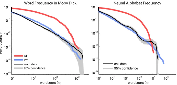
as city size, language, spike responses, etc., also exhibit power-law tails (Zipf, 1949; Newman, 2005). Figure 2 shows two such examples, along with a sample drawn from the best-fitting DP and PYP distributions.

Let PY(d, α) denote the PYP with discountparameterdandconcentrationparameterα(also called the “Dirichlet parameter”), ford∈[0,1), α >−d. Whend= 0, this reduces to the Dirichlet process, DP(α). To gain intuition for the DP and PYP, it is useful to consider typical samplesπ with weights {πi}sorted in decreasing order of probability, so that π(1)> π(2)>· · ·. The concentration parameterαcontrols how much of the probability mass is concentrated in the first few samples, that is, in the head instead of the tail of the sorted distribution. For smallαthe first few weights carry most of the probability mass whereas, for largeα, the probability mass is more spread out so thatπ is more uniform. As noted above the discount parameterdcontrols the shape of the tail. Largerd gives heavier power-law tails, whiled= 0 yields exponential tails.

We can draw samples π ∼PY(d, α) using an infinite sequence of independent Beta random variables in a process known as “stick-breaking” (Ishwaran and James, 2001)

βi∼Beta(1−d, α+id), ˜πi= i−1 Y

j=1

(1−βj)βi, (9)

where ˜πi is known as thei’thsize-biased permutationfromπ (Pitman, 1996). The ˜πisampled in this manner are not strictly decreasing, but decrease on average such thatP∞

i=1˜πi= 1 with probability 1 (Pitman and Yor, 1997).

1. Here, we will assume the base measure is non-atomic, so that the atomsφi’s are distinct with probability one.

This allows us to ignore the base measure, making entropy of the distribution equal to the entropy of the weights

π.

2. GEM stands for “Griffiths, Engen and McCloskey”, after three researchers who considered these ideas early on (Ewens, 1990).

Word Frequency in Moby Dick

100 101 102 103

10−5

10−4

10−3

10−2

10−1

100

P[wordcount > n]

word data 95% confidence DP

PY

wordcount (n) 10

0 ₁₀1 ₁₀2 ₁₀3 ₁₀4 ₁₀5

10−5

10−4

10−3

10−2

10−1

100

wordcount (n) cell data

95% confidence

Neural Alphabet Frequency

Figure 2: Empirical cumulative distribution functions of words in natural language (left) and neural spike patterns (right). We compare samples from the DP (red) and PYP (blue) priors for two data sets with heavy tails (black). In both cases, we compare the empirical CDF estimated from data to distributions drawn from DP and PYP using the ML values of αand (d, α) respectively. For both data sets, PYP better captures the heavy-tailed behavior of the data. (left)Frequency ofN= 217826 words in the novel Moby Dick by Herman Melville. (right)Frequencies amongN = 1.2×106 _{neural spike words from 27} simultaneously-recorded retinal ganglion cells, binarized and binned at 10ms.

3.1 Expectations over DP and PYP Priors

For our purposes, a key virtue of PYP priors is a mathematical property calledinvariance under size-biased sampling. This property allows us to convert expectations overπ on the infinite-dimensional simplex (which are required for computing the mean and variance of H given data) into one- or two-dimensional integrals with respect to the distribution of the first two size-biased samples (Perman et al., 1992; Pitman, 1996).

Proposition 1 (Expectations with first two size-biased samples) Forπ∼PY(d, α),

E(π|d,α) "∞

X

i=1 f(πi)

#

=_E(˜π1|d,α)

_f(˜π 1) ˜ π1

, (10)

E(π|d,α) 

 X

i,j6=i

g(πi, πj) 

=E(˜π1,π˜2|d,α)

_g(˜π 1,˜π2) ˜ π1˜π2

(1−π˜1)

, (11)

whereπ˜1 andπ˜2 are the first two size-biased samples from π.

The first result (10) appears in (Pitman and Yor, 1997), and an analogous proof can be constructed for (11) (see Appendix).

The direct consequence of this proposition is that the first two moments ofH(π) under the PYP and DP priors have closed forms4

E[H|d, α] =ψ0(α+ 1)−ψ0(1−d), (12)

var[H|d, α] = α+d (α+ 1)2_(1−d)+

1−d

α+ 1ψ1(2−d)−ψ1(2 +α). (13)

The derivation can be found in the Appendix.

3.2 Expectations over DP and PYP Posteriors

A useful property of PYP priors (for multinomial observations) is that the posterior p(π|x, d, α) takes the form of a mixture of a Dirichlet distribution (over the observed symbols) and a Pitman-Yor process (over the unobserved symbols) (Ishwaran and James, 2003). This makes the integrals over the infinite-dimensional simplex tractable and, as a result, we obtain closed-form solutions for the posterior mean and variance ofH. LetK be the number of unique symbols observed inN samples, i.e.,K=PA

i=11{ni>0}.

5 _{Further, letαi=ni−d,N =}P

ni, andA=P

αi=P

ini−Kd=N−Kd. Now, following Ishwaran and colleagues (Ishwaran and Zarepour, 2002), we write the posterior as an infinite random vectorπ|x, d, α= (p1, p2, p3, . . . , pK, p∗π0), where

(p1, p2, . . . , pK, p∗)∼Dir(n1−d, . . . , nK−d, α+Kd) (14) π0 := (π1, π2, π3, . . .)∼PY(d, α+Kd).

The posterior mean E[H|x, d, α] is given by

E[H|α, d,x] =ψ0(α+N+ 1)−

α+Kd

α+N ψ0(1−d)− 1 α+N

"K X

i=1

(ni−d)ψ0(ni−d+ 1) #

. (15)

The variance, var[H|x, d, α], may also be expressed in an easily-computable closed-form. As we discuss in detail in Appendix A.4, var[H|x, d, α] may be expressed in terms of the first two moments ofp∗,π, andp= (p1, . . . , pK) appearing in the posterior (14). Applying the law of total variance and using the independence properties of the posterior, we find

var[H|d, α] =Ep∗[(1−p∗)

2_{] var}

p [H(p)] +Ep∗[p 2

∗] var_π [H(π)] +_Ep∗[Ω

2_(p

∗)]−Ep∗[Ω(p∗)]

2_,

where Ω(p∗) = (1−p∗)Ep[H(p)]+p∗Eπ[H(π)]+H(p∗), andH(p∗) =−p∗log(p∗)−(1−p∗) log(1−p∗). To specify Ω(p∗), we letA=Ep[H(p)],B=Eπ[H(π)] so that

E[Ω] =Ep∗[1−p∗]Ep[H(p)] +Ep∗[p∗]Eπ[H(π)] +H(p∗),

E[Ω2] = 2Ep∗[p∗H(p∗)][B−A] + 2AEp∗[H(p∗)] +Ep∗[h

2_(p

∗)] +_Ep∗[p

2

∗]

B2−2AB

+ 2_Ep∗[p∗]AB+Ep∗[(1−p∗)

2_]A2_.

4. Entropy Inference under DP and PYP priors

The posterior expectations computed in Section 3.2 provide a class of entropy estimators for distribu-tions with countably-infinite support. For each choice of (d, α),E[H|α, d,x] is the posterior mean

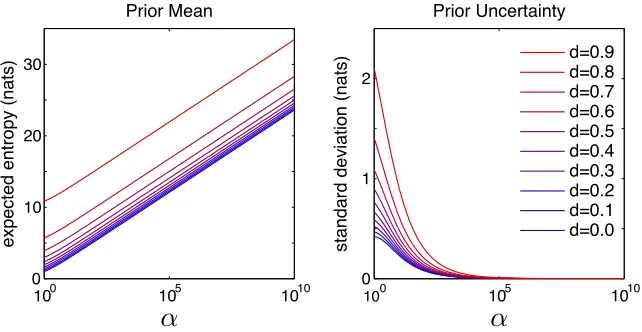
under aP Y(d, α) prior, analogous to the fixed-αDirichlet priors discussed in Section 2.2. Unfortu-nately, fixedP Y(d, α) priors carry the same difficulties as fixed Dirichlet priors. A fixed-parameter PY(d, α) prior onπ results in a highly concentrated prior distribution on entropy (Figure 3).

We address this problem by introducing a mixture prior p(d, α) on PY(d, α) under which the implied prior on entropy is flat.6 _{We then define the BLS entropy estimator under this mixture prior,}

5. We note that the quantityKhas been studied in Bayesian nonparametrics in its own right, for instance to study species diversity in ecological applications (Favaro et al., 2009).

6. Notice, however, that by constructing a flat prior on entropy, we do not obtain an objective prior. Here, we are not interested in estimating the underlying high-dimensional probabilities{πi}, but rather in estimating a single

100 105 1010 0

10 20 30

Prior Mean

expected entropy (nats)

100 105 1010

0 1 2

Prior Uncertainty

standard deviation (nats)

d=0.9 d=0.8 d=0.7 d=0.6 d=0.5 d=0.4 d=0.3 d=0.2 d=0.1 d=0.0

Figure 3: Prior entropy mean and variance (12) and 13 as a function ofαandd. Note that entropy is approximately linear in logα. For large values ofα,p(H(π)|d, α) is highly concentrated around the mean.

the Pitman-Yor Mixture (PYM) estimator, and discuss some of its theoretical properties. Finally, we turn to the computation of PYM, discussing methods for sampling, and numerical quadrature integration.

4.1 Pitman-Yor Process Mixture (PYM) Prior

One way of constructing a flat mixture prior is to follow the approach of Nemenman and colleagues (Nemenman et al., 2002), settingp(d, α) proportional to the derivative of the expected entropy (12).

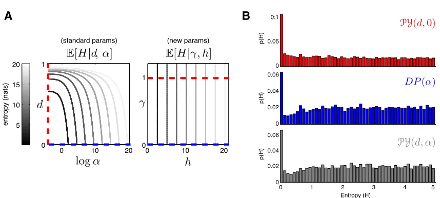
Unlike NSB, we have two parameters through which to control the prior expected entropy. For instance, large prior (expected) entropies can arise either from large values ofα(as in the DP) or from values ofdnear 1 (see Figure 3A). We can explicitly control this trade-off by reparameterizing PYP as follows

h=ψ0(α+ 1)−ψ0(1−d), γ=

ψ0(1)−ψ0(1−d) ψ0(α+ 1)−ψ0(1−d)

,

whereh >0 is equal to the expected prior entropy (12), andγ∈[0,∞) captures prior beliefs about tail behavior (Figure 4A). Forγ= 0, we have the DP (i.e.,d= 0, givingπ with exponential tails), while for γ= 1 we have a PY(d,0) process (i.e., α= 0, yieldingπ with power-law tails). In the limit whereα→ −1 andd→1, γ→ ∞. Where required, the inverse transformation to standard PY parameters is given by: α=ψ0−1(h(1−γ) +ψ0(1))−1,d= 1−ψ0−1(ψ0(1)−hγ),whereψ0−1(·) denotes the inverse digamma function.

We can construct an approximately flat improper distribution over H on [0,∞] by setting p(h, γ) =q(γ) for allh, whereqis any density on [0,∞). We call this the Pitman-Yor process mixture (PYM) prior. The induced prior on entropy is thus

p(H) = Z Z

p(H|π)p(π|γ, h)p(γ, h) dγdh,

0 10 20 0

1

entropy (nats) 5 10 15 20

0 10 20

0 1

(standard params) (new params)

0 0.05

0.1

p(H)

0 0.02 0.04 0.06

p(H)

0 1 2 3 4

0 0.02 0.04 0.06

Entropy (H)

p(H)

A

B

5

Figure 4: Prior over expected entropy under Pitman-Yor process prior. (A) Left: expected entropy as a function of the natural parameters (d, α). Right: expected entropy as a function of transformed parameters (h, γ). The dotted red and blue lines indicate the contours on which the PY(d,0) and DP(α) priors are defined, respectively. (B) Sampled prior distributions (N = 5e3) over entropy implied by three different PYM priors, each with a different mixing density over α andd. We formulate each prior in the transformed parametersγ andh. We place a uniform prior onhand show three different choices of prior q(γ). Each resulting PYM prior is a mixture of Pitman-Yor processes: PY(d,0) (red) uses a mixing density overd: q(γ) =δγ−1; PY(0, α) = DP(α) (blue) uses a mixing density over α: q(γ) =δγ; and PY(d, α) (grey) uses a mixture over both hyperparameters: q(γ) = exp(− 10

1−γ)1{γ<1}. Note that for all of these examples, the “true” p(H) is an improper prior supported on [0,∞). We visualize the sampled distributions only on the range from 0 to 5 nats, since sampling from PY becomes prohibitively expensive with increasing expected entropy (especially asd→1).

intervals and higher estimates of entropy. PYM mixture priors resulting from different choices of q(γ) are all approximately flat onH, but each favors distributions with different tail behavior; the ability to selectq(γ) greatly enhances the flexibility of PYM, allowing the practitioner to adapt it to her own data.

Figure 4B shows samples from this prior under three different choices of q(γ), forh uniform on [0,3]. For the experiments, we use q(γ) = exp(− 10

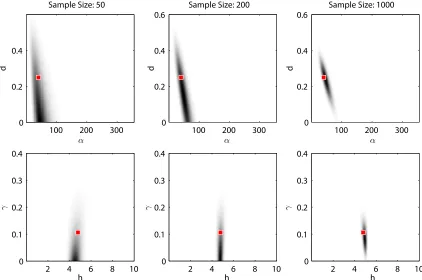
1−γ)1{γ<1} which yields good results by weighting less on extremely heavy-tailed distributions.7 _{Combined with the likelihood, the posterior} p(d, α|x)∝p(x|d, α)p(d, α) quickly concentrates as more data are given (see Figure 5).

4.2 The Pitman-Yor Mixture Entropy Estimator

Now that we have determined a prior on the infinite simplex, we turn to the problem of inference given observationsx. The Bayes least squares entropy estimator under the mixture priorp(d, α), the

d

Sample Size: 50

100 200 300 0

0.2 0.4

h

2 4 6 8 10

0 0.1 0.2 0.3 0.4

d

Sample Size: 200

100 200 300 0

0.2 0.4 0.6

2 4 6 8 10

0 0.1 0.2 0.3 0.4

d

Sample Size: 1000

100 200 300 0

0.2 0.4 0.6

2 4 6 8 10

0 0.1 0.2 0.3 0.4

h h

Figure 5: Convergence ofp(d, α|x) for increasing sample size. Both parameterization (d, α) and (γ, h) are shown. Data are simulated from a PY(0.25,40) whose parameters are indicated by the red dot.

Pitman-Yor Mixture (PYM) estimator, takes the form

ˆ

HPYM=E[H|x] =

Z

E[H|x, d, α]

p(x|d, α)p(d, α)

p(x) d(d, α), (16)

where E[H|x, d, α] is the expected posterior entropy for a fixed (d, α) (see Section 3.2). The quantity

p(x|d, α) is the evidence, given by

p(x|d, α) =

_QK−1

l=1 (α+ld) QK

i=1Γ(ni−d)

Γ(1 +α)

Γ(1−d)K_Γ(α+N) . (17)

We can obtain posterior credible intervals for ˆHPYMby estimating the posterior varianceE[(H−

ˆ

HPYM)2|x]. The estimate takes the same form as (16), except that we replaceE[H|x, d, α] with

var[H|x, d, α] in the integrand.

4.3 Computation

cost. Then, we outline a fast method for performing the numerical integration over a suitable range ofαandd.

4.3.1 Multiplicities

We can compute the expected entropy E[H|x, d, α] more efficiently by using a representation in

terms of multiplicities, a compressed statistic often used under other names (e.g., the empirical histogram distribution function as discussed by Paninski 2003). Multiplicities are the number of symbols that have occurred with a given frequency in the sample. Lettingmk =|{i:ni =k}|denote the total number of symbols with exactlyk observations in the sample gives the compressed statistic m= [m0, m1, . . . , mM]

>

, whereM is the largest number of samples for any symbol. Note that the dot product [0,1, . . . , M]>m=N, is the total number of samples.

The multiplicities representation significantly reduces the time and space complexity of our computations for most data sets as we need only compute sums and products involving the number of symbols with distinct frequencies (at mostM), rather than the total number of symbolsK. In practice we compute all expressions not explicitly involvingπusing the multiplicities representation. For instance, when expressed in terms of the multiplicities the evidence takes the compressed form

p(x|d, α) =p(m1, . . . , mM|d, α) =Γ(1 +α)

QK−1

l=1 (α+ld) Γ(α+N)

M Y

i=1 _Γ(i

−d) i!Γ(1−d)

mi _M! mi!.

4.3.2 Heuristic for Integral Computation

In principle the PYM integral over αis supported on the range [0,∞). In practice, however, the posterior concentrates on a relatively small region of parameter space. It is generally unnecessary to consider the full integral over a semi-infinite domain. Instead, we select a subregion of [0,1]×[0,∞) which supports the posterior up toprobability mass. The posterior is unimodal in each variable αanddseparately (see Appendix D); however, we do not have a proof for the unimodality of the evidence. Nevertheless, if there are multiple modes, they must lie on a strictly decreasing line ofdas a function ofαand, in practice, we find the posterior to be unimodal. We illustrate the concentration of the evidence visually in Figure 5.

We compute the hessian at the MAP parameter value, (dMAP, αMAP). Using the inverse hessian as the covariance of a Gaussian approximation to the posterior, we select a grid spanning±6 std. We use numerical integration (Gauss-Legendre quadrature) on this region to compute the integral. When the hessian is rank-deficient (which may occur, for instance, when theαMAP= 0 ordMAP= 0), we use Gauss-Legendre quadrature to perform the integral indover [0,1), but employ a Fourier-Chebyshev numerical quadrature routine to integrateαover [0,∞) (Boyd, 1987).

4.4 Sampling the Full Posterior OverH

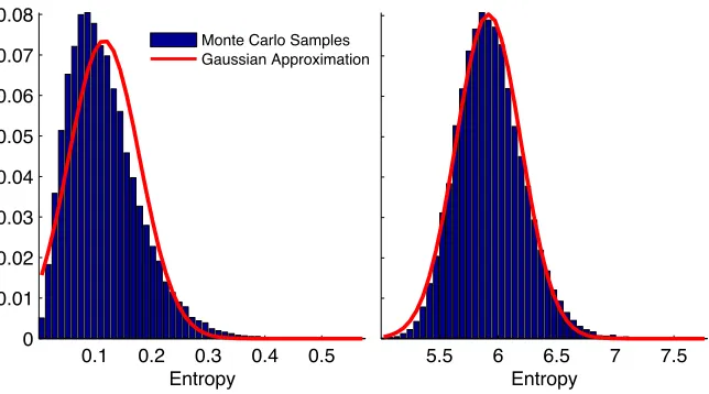
The closed-form expressions for the conditional moments derived in the previous section allow us to compute PYM and its variance by 2-dimensional numerical integration. PYM’s posterior mean and variance provide, essentially, a Gaussian approximation to the posterior, and corresponding credible regions. However, in some situations (see Figure 6), variance-based credible intervals are a poor approximation to the true posterior credible intervals. In these cases we may wish to examine the full posterior distribution overH.

0.1 0.2 0.3 0.4 0.5 0

0.01 0.02 0.03 0.04 0.05 0.06 0.07 0.08

Entropy

Monte Carlo Samples Gaussian Approximation

5.5 6 6.5 7 7.5

Entropy

Figure 6: The posterior distributions of entropy for two data sets of 100 samples drawn from distinct distributions and the Gaussian approximation to each distribution based upon the posterior mean and variance. (left) Simulated example with low entropy. Notice that the true posterior is highly asymmetric, and that the Gaussian approximation does not respect the positivity of H. (right) Simulated example with higher entropy. The Gaussian approximation is a much closer approximation to the true distribution.

accuracy.8 Even so, samplingπ∼PY(d, α) fordnear 1, where π is likely to be heavy-tailed, may require intractably large number of samples to obtain a good approximation.

We address this problem by directly estimating the entropy of the tail, PY(d, α+Nsd), using (12). As shown in Figure 3, the prior variance of PY becomes arbitrarily small as for largeα. We need only enough samples to assure that the variance of the tail entropy is small. The resulting final sample is the entropy of the (finite) samples plus the expected entropy of the tail,H(π∗_{) +}

E[H|d, α+Kd].9

Sampling entropy is most useful for very small amounts of data drawn from distributions with low expected entropy. In Figure 5 we illustrate the posterior distributions of entropy in two simulated experiments. In general, as the expected entropy and sample size increase, the posterior becomes more approximately Gaussian.

5. Theoretical Properties of PYM

Having defined PYM and discussed its practical computation, we now establish conditions under which (16) is defined (i.e., the right–hand of the equation is finite), and also prove some basic facts about its asymptotic properties. While ˆHPYMis a Bayesian estimator, we wish to build connections to the literature by showing frequentist properties.

Note that the prior expectation _E[H] does not exist for the improper prior defined above, since p(h=_E[H])∝1 on [0,∞]. It is therefore reasonable to ask what conditions on the data are sufficient to obtain finite posterior expectation ˆHPYM=E[H|x]. We give an answer to this question in the following short proposition (proofs of all statements may be found in the appendix),

8. Bounds on the number of samples necessary to reachon average have been considered by Ishwaran and James (2001).

Theorem 2 Given a fixed data setxofN samples,HPYMˆ <∞for any prior distribution p(d, α)if N−K≥2.

In other words, we require 2 coincidences in the data for ˆHPYM to be finite. When no coincidences have occurred inx, we have no evidence regarding the support of theπ and our resulting entropy estimate is unbounded. In fact, in the absence of coincidences, no entropy estimator can give a reasonable estimate without prior knowledge or assumptions aboutA.

Concerns about inadequate numbers of coincidences are peculiar to the under-sampled regime; asN → ∞, we will almost surely observe each letter infinitely often. We now turn to asymptotic considerations, establishing consistency of ˆHPYM in the limit of largeN for a broad class of distri-butions. It is known that the plugin is consistent for any distribution (finite or countably infinite), although the rate of convergence can be arbitrarily slow (Antos and Kontoyiannis, 2001). Therefore, we establish consistency by showing asymptotic convergence to the plugin estimator.

For clarity, we explicitly denote a quantity’s dependence upon sample size N by introducing a subscript. ThusxandKbecomexN andKN respectively. As a first step we show thatE[H|xN, d, α] converges to the plugin estimator.

Theorem 3 AssumingxN drawn from a fixed, finite or countably infinite discrete distribution π such that KN

N P −→0

|_E[H|xN, d, α]−E[Hplugin|xN]| P −→0

The assumption KN/N→0 is more general than it may seem. For any infinite discrete distribution it holds thatKN →E[KN] a.s. andE[KN]/N →0 a.s. (Gnedin et al., 2007). Hence,KN/N→0 in

probability for an arbitrary distribution. As a result, the right–hand–side of (15) shares its asymptotic behavior, in particular consistency, with ˆHplugin. As (15) is consistent for each value ofαandd, it is intuitively plausible that ˆHPYM, as a mixture of such values, should be consistent as well. However, while (15) alone is well-behaved, it is not clear that ˆHPYM should be. SinceE[H|x, d, α]→ ∞as

α→ ∞, care must be taken when integrating overp(d, α|x). Our main consistency result is, Theorem 4 For any proper prior or bounded improper prior p(d, α), if dataxN are drawn from a fixed, countably infinite discrete distributionπ such that for some constant C >0 KN =o(N1−1/C)

in probability, then

|_E[H|xN]−E[Hplugin|xN]| P −→0

Intuitively, the asymptotic behavior of KN/N is tightly related to the tail behavior of the distribution (Gnedin et al., 2007). In particular,KN ∼cNb with 0< b <1 if and only ifπi∼c0i

1

b

wherec andc0 are constants, and we assumeπi is non-increasing (Gnedin et al., 2007). The class of distributions such thatKN =o(N1−1/C_{) a.s. includes the class of power-law or thinner tailed} distributions, i.e.,πi=O(ib_{) for someb >1 (again πi is assumed non-increasing).}

While consistency is an important property for any estimator, we emphasize that PYM is designed to address the under-sampled regime. Indeed, since ˆHpluginis consistent and has an optimal rate of convergence for a large class of distributions (Vu et al., 2007; Antos and Kontoyiannis, 2001; Zhang, 2012), asymptotic properties provide little reason to use ˆHPYM. Nevertheless, notice that Theorem 4 makes very weak assumptions aboutp(d, α). In particular, the result is not dependent upon the form of the PYM prior introduced in the previous section; it holds for any probability distributionp(d, α), or even a bounded improper prior. Thus, we can view Theorem 4 as a statement about a class of PYM estimators. Almost any prior we choose on (d, α) results in a consistent estimator of entropy.

6. Simulation Results

100 600 3900 25000 5

6 7 8 9

PY (1000, 0)

Entropy (nats)

100 600 3900 25000

5 6 7 8 9

PY (1000, 0.1)

Entropy (nats)

100 600 3900 25000

4.5 5 5.5 6 6.5

PY (1000, 0.4)

Entropy (nats)

DPM NSB (K = 105₎ PYM

CAE ANSB Zhang plugin MiMa GR08

A

B

C

# of samples # of samples

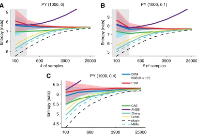
Figure 7: Comparison of estimators on stick-breaking distributions. Poisson-Dirichlet distribution with (d= 0, α= 1000) (A), (d= 0.1, α= 1000) (B), (d= 0.4, α= 100) (C). Recall that the Dirichlet Process is the Pitman-Yor Process withd= 0. We compare our estimators (DPM, PYM) with other enumerable support estimators (CAE, ANSB, Zhang, GR08), and finite support estimators (plugin, MiMa). Note that in these examples, the DPM estimator performs indistinguishably from NSB with alphabet size A fixed to a large value (A= 105_{). For the experiments, we first sample a singleπ ∼PY(d, α) using the} stick-breaking procedure of (9). For eachN (x-axis), we apply all estimators to each of 10 sample data sets drawn randomly fromπ. Solid lines are averages over all 10 realizations. Colored shaded area represent 95% credible intervals averaged over all 10 realizations. Gray shaded area represents the ANSB approximation regime defined as expected number of unique symbols being more than 90% the total number of samples.

our estimators, DPM (d= 0 only) and PYM ( ˆHPYM), with other enumerable-support estimators: coverage-adjusted estimator (CAE) (Chao and Shen, 2003; Vu et al., 2007), asymptotic NSB (ANSB, Section 2.4) (Nemenman, 2011), Grassberger’s asymptotic bias correction (GR08) (Grassberger, 2008), and Good-Turing estimator (Zhang, 2012). Note that similar to ANSB, DPM is an asymptotic (Poisson-Dirichlet) limit of NSB, and hence in practice behaves identically to NSB with large but finite K. We also compare with plugin (3) and a standard Miller-Maddow (MiMa) bias correction method with a conservative assumption that the number of uniquely observed symbols is K (Miller, 1955). To make comparisons more straightforward, we do not apply additional bias correction methods (e.g., jackknife) to any of the estimators.

10 60 300 2500 15000 100000 0.5

1 1.5 2

Power−law with [exponent 1.5]

# of samples

Entropy (nats)

# of samples

10 60 300 10000

1 1.5 2

Power−law with [exponent 2]

Entropy (nats)

DPM/NSB PYM

CAE ANSB Zhang

plugin MiMa GR08

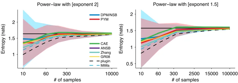
Figure 8: Comparison of estimators on power-law distributions. The highest probabilities in these power-law distributions were large enough that they were never effectively under-sampled.

The experiments of Figure 7 show performance on a singleπ∼PY(d, α) drawn using the stick-breaking procedure of (9). We drawπi according to (9) in blocks of size 103until 1−PNsπi <10

−3_, where Ns is the number of sticks. Unsurprisingly, PYM performs well when the data are truly generated by a Pitman-Yor process (Figure 7). Credible intervals for DPM tend to be smaller than PYM, although both shrink quickly (indicating high confidence). When the tail of the distribution is exponentially decaying, (d= 0 case; Figure 7 top), DPM shows slightly improved performance. When the tail has a strong power-law decay, (Figure 7 bottom), PYM performs better than DPM. Most of the other estimators are consistently biased down, with the exception of ANSB.

The shaded gray area indicates the ANSB approximation regime, where the approximation used to define the ANSB estimator is approximately valid. Although this region has no definitive boundary, it corresponds to a regime where where the average number of coincidences is small relative to the number of samples. Following Nemenman (2011), we define the under-sampled regime to be the region whereE[KN]/N >0.9, whereKN is the number of unique symbols appearing in a sample of size N. Note that only 3 out of 10 results in Figures. 7, 8, 9, 10 have shaded area; the ANSB approximation regime is not large enough to appear in the plots. This regime appears to be designed for a relatively broad distribution (close to uniform distribution). In cases where a single symbol has high probability, the ANSB approximation regime is essentially never valid. In our example distributions, this is the case with for power-law distributions andPYdistributions with larged. For example, Figure 8 is already outside of the ANSB approximation regime with only 4 samples.

Although Pitman-Yor process PY(d, α) has a power-law tail controlled byd, the high probability portion is modulated by α and does not strictly follow a power-law distribution as a whole. In Figure 8, we evaluate the performance for pi ∝i−2 _{and pi ∝i}−1.5_{. PYM and DPM have slight} negative biases, but the credible interval covers the true entropy for all sample sizes. For small sample sizes, most estimators are negatively biased, again except for ANSB (which does not show up in the plot since it is severely biased upwards). Notably, CAE performs very well in moderate sample sizes.

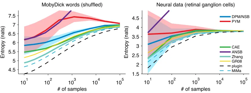
In Figure 9 we compute the entropy per word of in the novel Moby Dick by Herman Melville and entropy per time bin of a population of retinal ganglion cells from monkey retina (Pillow et al., 2005). We tokenized the novel into individual words using the Python library NLTK.10Punctuation is disregarded. These real-world data sets have heavy, approximately power-law tails11_{as pointed out}

10. Further information about the Natural Language Toolkit (NLTK) may be obtained at the project’s website,

http://www.nltk.org/.

4.5 5 5.5 6 6.5 7 7.5

MobyDick words (shuffled)

Entropy (nats)

101 102 103 104 105

# of samples 10

1 ₁₀2 ₁₀3 ₁₀4 ₁₀5

1.5 2 2.5 3 3.5 4 4.5

Neural data (retinal ganglion cells)

# of samples

Entropy (nats)

DPM/NSB PYM

CAE ANSB Zhang plugin MiMa GR08

Figure 9: Comparison of estimators on real data sets.

earlier in Figure 2. For Moby Dick, PYM slightly overestimates, while DPM slightly underestimates, yet both methods are closer to the entropy estimated by the full data available than other estimators. DPM is overly confident (its credible interval is too narrow), while PYM becomes overly confident with more data. The neural data were preprocessed to be a binarized response (10 ms time bins) of 8 simultaneously recorded off-response retinal ganglion cells. PYM, DPM, and CAE all perform well on this data set with both PYM and DPM bracketing the asymptotic value with their credible intervals.

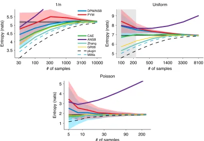
Finally, we applied the denumerable-support estimators to finite-support distributions (Figure 10). The power-law pn∝n−1 has the heaviest tail among the simulations we consider but notice that it does not define a proper distribution (the probability mass does not integrate), and so we use a truncated 1/ndistribution with the first 1000 symbols (Figure 10 top). Initially PYM shows the least bias, but DPM provides a better estimate for increasing sample size. However, notice that for both estimates the credible intervals consistently cover the true entropy. Interestingly, the finite support estimators perform poorly compared to DPM, CAE and PYM. For the uniform distribution over 1000 symbols, both DPM and PYM have slight upward bias, while CAE shows almost perfect performance (Figure 10 middle). For Poisson distribution, a theoretically enumerable-support distribution on the natural numbers, the tail decays so quickly that the effective support (due to machine precision) is very small (26 in this case). All the estimators, with the exception of ANSB, work quite well.

The novel Moby Dick provides the most challenging data: no estimator seems to have converged, even with the full data. Surprisingly, the Good-Turing estimator (Zhang, 2012) tends to perform similarly to the Grassberger and Miller-Maddow correction methods. Among such the bias-correction methods, Grassberger’s method tended to show the best performance, outperforming Zhang’s method.

5 10 30 90 200 1

2 3 4 5

Poisson

# of samples

Entropy (nats)

100 200 500 1400 3300 8100

5 6 7 8 9

Uniform

Entropy (nats)

# of samples

30 100 300 1000 3100 10000

3.5 4 4.5 5 5.5

1/n

Entropy (nats)

DPM/NSB PYM

CAE ANSB Zhang plugin MiMa GR08

# of samples

Figure 10: Comparison of estimators on finite support distributions. Black solid line indicates the true entropy. Poisson distribution (λ=e) has a countably infinite (but very thin) tail. All probability mass was concentrated on 26 symbols, within machine precision.

7. Conclusion

In this paper we introduced PYM, a new entropy estimator for distributions with unknown support. We derived analytic forms for the conditional mean and variance of entropy under a DP and PY prior for fixed parameters. Inspired by the work of Nemenman et al. (2002), we defined a novel PY mixture prior, PYM, which implies an approximately flat prior on entropy. PYM addresses two major issues with NSB: its dependence on knowledge ofAand its inability (inherited from the Dirichlet distribution) to account for the heavy-tailed distributions which abound in biological and other natural data.

Further experiments on diverse data sets might reveal ways to improve PYM, such as new tactics or theory for selecting the prior on tail behavior,q(γ). It may also prove fruitful to investigate ways to tailor PYM to a specific application, for instance by combining it with with more structured priors such as those employed by Archer et al. (2013). Further, while we have shown that PYM is consistent for any prior, an expanded theory might investigate the convergence rate, perhaps in relation to the choice of prior.

101 102 103 104 105 10−2

100

# of samples

Computation time (sec)

DPM PYM

CAE ANSB Zhang plugin GR08

Figure 11: Median computation time to estimate entropy for the neural data. The computation time excludes the preprocessing required to build the histogram and convert to multiplicity representation. Note that for DPM and PYM this time also includes estimating the posterior variance.

Acknowledgments

We thank E. J. Chichilnisky, A. M. Litke, A. Sher and J. Shlens for retinal data, and Y. W. Teh and A. Cerquetti for helpful comments on the manuscript. This work was supported by a Sloan Research Fellowship, McKnight Scholar’s Award, and NSF CAREER Award IIS-1150186 (JP). Parts of this manuscript were presented at the Advances in Neural Information Processing Systems (NIPS) 2012 conference.

Appendix A. Derivations of Dirichlet and PY Moments

In this Appendix we present as propositions a number of technical moment derivations used in the text.

A.1 Mean Entropy of Finite Dirichlet

Proposition 5 (Replica trick for entropy [Wolpert and Wolf, 1995])

Forπ∼Dir(α1, α2, . . . , αA), such that PAi=1αi=A, and letting ~α= (α1, α2, . . . , αA), we have

E[H(π)|α~] = ψ0(A+ 1)− A X

i=1 αi

Aψ0(αi+ 1) (18)

Proof First, letcbe the normalizer of Dirichlet,c= Q

jΓ(αj)

Γ(A) and letLdenote the Laplace transform (onπtos). Now we have that

cE[H|α~] =

Z

−X i

πilog2πi !

δ(P iπi−1)

Y

j παj−1

j dπ

=−X

i Z

(παi

i log2πi)δ(Piπi−1) Y

j6=i παj−1

=−X i

Z _d

d(αi)π αi i

δ(P

iπi−1) Y

j6=i παj−1

j dπ

=−X

i d d(αi)

Z παi

i δ(Piπi−1) Y

j6=i παj−1

j dπ

=−X

i d d(αi)L

−1 

L(π αi i )

Y

j6=i

L(παj−1

j )



(1)

=−X

i d d(αi)L

−1

_{Γ(αi+ 1)}Q

j6=iΓ(αj) sPk(αk)+1

(1)

=−X

i d d(αi)

_{Γ(αi+ 1)} Γ(P

k(αk) + 1)

Y

j6=i Γ(αj)

=−X

i

Γ(αi+ 1) Γ(P

kαk+ 1)

[ψ0(αi+ 1)−ψ0(A+ 1)] Y

j6=i Γ(αj)

= "

ψ0(A+ 1)− A X

i=1 αi

Aψ0(αi+ 1) # Q

jΓ(αj) Γ(A) .

A.2 Variance of Entropy for Finite Dirichlet

We deriveE[H2(π)|~α]. In practice we compute var[H(π)|~α] =E[H2(π)|~α]−E[H(π)|~α]2.

Proposition 6 Forπ∼Dir(α1, α2, . . . , αA), such thatPAi=1αi=A, and letting~α= (α1, α2, . . . , αA),

we have

E[H2(π)|α~] =

X

i6=k

αiαk

(A+ 1)(A)Iik+ X

i

αi(αi+ 1)

(A+ 1)(A)Ji (19)

Iik= (ψ0(αk+ 1)−ψ0(A+ 2)) (ψ0(αi+ 1) −ψ0(A+ 2))−ψ1(A+ 2)

Ji= (ψ0(αi+ 2)−ψ0(A+ 2))2+ψ1(αi+ 2) −ψ1(A+ 2)

Proof We can evaluate the second moment in a manner similar to the mean entropy above. First, we split the second moment into square and cross terms. To evaluate the integral over the cross terms, we apply the “replica trick” twice. Lettingc be the normalizer of Dirichlet,c=

Q jΓ(αj)

Γ(A) we have

c_E[H2|α~] = Z

−X i

πilog2πi !2

δ(P iπi−1)

Y

j παj−1

j dπ

=X

i Z

π_i2log₂2πiδ(P iπi−1)

Y

j παj−1

j dπ

+X

i6=k Z

(πilog2πi) (πklog2πk)δ(Piπi−1) Y

j παj−1

=X i

Z παi+1

i log2 2_π

iδ(Piπi−1) Y

j6=i παj−1

j dπ

+X

i6=k Z

(παi

i log2πi) (π αk

k log2πk)δ(Piπi−1) Y

j6∈{i,k} παj−1

j dπ

=X

i

d2 d(αi+ 1)2

Z παi+1

i δ(Piπi−1) Y

j6=i παj−1

j dπ

+X

i6=k d dαi

d dαk

Z (παi

i ) (π αk k )δ(

P iπi−1)

Y

j6∈{i,k} παj−1

j dπ

Assumingi6=k, these will be the cross terms.

Z

(πilog2πi)(πklog2πk)δ(Piπi−1) Y

j παj−1

j dπ = d dαi d dαk Z (παi

i )(π αk

k )δ(Piπi−1) Y

j6∈{i,k} παj−1

j dπ

= d

dαi d dαk

_{Γ(αi+ 1)Γ(αk+ 1)} Γ(A+ 2)

Y

j6∈{i,k} Γ(αj)

= d

dαk _α

iΓ(αk+ 1)

Γ(A+ 2) ψ0(αi+ 1) −αiΓ(αk+ 1)

Γ(A+ 2) ψ0(A+ 2)

Y

j6=k Γ(αj)

= d

dαk _α

iψ0(αk+ 1)

Γ(A+ 2) ψ0(αi+ 1) −αiΓ(αk+ 1)

Γ(A+ 2) ψ0(A+ 2)

Y

j6=k Γ(αj)

= αiαk

Γ(A+ 2)[(ψ0(αk+ 1)−ψ0(A+ 2)) (ψ0(αi+ 1)−ψ0(A+ 2))−ψ1(A+ 2)]

Y

j Γ(αj)

= αiαk

(A+ 1)(A)[(ψ0(αk+ 1)−ψ0(A+ 2)) (ψ0(αi+ 1)−ψ0(A+ 2))−ψ1(A+ 2)]

Q jΓ(αj) Γ(A)

d2 d(αi+ 1)2

Z παi+1

i δ(Piπi−1) Y

j6=i παj−1

j dπ

= d

2 d(αi+ 1)2

_Γ(α i+ 2) Γ(A+ 2)

Y

j6=i Γ(αj)

= d 2 dz2

_{Γ(z+ 1)} Γ(z+c)

Y

j6=i

=Γ(1 +z)

Γ(c+z)[(ψ0(1 +z)−

ψ0(c+z))2+ψ1(1 +z)−ψ1(c+z) Y j6=i

Γ(αj)

= z(z−1) (c+z−1)(c+z−2)

(ψ0(1 +z)−ψ0(c+z))2

+ψ1(1 +z)−ψ1(c+z)] Q

jΓ(αj) Γ(A) =(αi+ 1)(αi)

(A+ 1)(A)

(ψ0(αi+ 2)−ψ0(A+ 2))2+ψ1(αi+ 2)

−ψ1(A+ 2)] Q

jΓ(αj) Γ(A)

Summing over all terms and adding the cross and square terms, we recover the desired expression for_E[H2_(π)|~α].

A.3 Prior Entropy Mean and Variance Under PY

We derive the prior entropy mean and variance of a PY distribution with fixed parameters αandd,

Eπ[H(π)|d, α] and varπ[H(π)|d, α]. We first prove our Proposition 1 (mentioned in (Pitman and

Yor, 1997)). This proposition establishes the identityE

h P∞

i=1f(πi) α

i =R1

0 f(˜π1)

˜

π1 p(˜π1|α)dπ˜1 which

will allow us to compute expectations over PY using only the distribution of the first size biased sample, ˜π1.

Proof[Proof of Proposition 1]

First we validate (10). Writing out the general form of the size-biased sample

p(˜π1=x|π) =

∞ X

i=1

πiδ(x−πi),

we see that

E˜π1

_f(˜π 1) ˜ π1

=

Z 1 0

f(x)

x p(˜π1=x)dx =

Z 1 0

Eπ

_f(x)

x p(˜π1=x|π)

dx

= Z 1

0

Eπ

"_∞ X

i=1 f(x)

x πiδ(x−πi) #

dx

=_Eπ

" Z 1

0

∞ X

i=1 f(x)

x πiδ(x−πi)dx #

=_Eπ "∞

X

i=1 Z 1

0 f(x)

x πiδ(x−πi)dx #

=Eπ

"∞ X

i=1 f(πi)

#

,

A similar method validates (11). We will need the second size-biased sample in addition to the first. We begin with the sum inside the expectation on the left–hand side of (11)

X

i X

j6=i

g(πi, πj) (20)

= P

i P

j6=ig(πi, πj) p(˜π1=πi,π˜2=πj)

p(˜π1=πi,π˜2=πj) (21)

=X

i X

j6=i

g(πi, πj)

πiπj (1−πi)p(˜π1=πi,π˜2=πj) (22) =Eπ˜1,˜π2

g(˜π1,π˜2) ˜ π1˜π2

(1−π˜1) π

(23)

where the joint distribution of size biased samples is given by

p(˜π1=πi,˜π2=πj) =p(˜π1=πi)p(˜π2=πj|˜π1=πi) =πi·

πj 1−πi

As this identity is defined for any additive functionalf ofπ, we can employ it to compute the first two moments of entropy. For PYP (and DP whend= 0), the first size-biased sample is distributed according to

˜

π1∼Beta(1−d, α+d) (24)

Proposition 1 gives the mean entropy directly. Taking f(x) =−xlog(x) we have

E[H(π)|d, α] =−Eα[log(π1)] =ψ0(α+ 1)−ψ0(1−d),

The same method may be used to obtain the prior variance, although the computation is more involved. For the variance, we will need the second size-biased sample in addition to the first. The second size-biased sample is given by,

˜

π2= (1−π˜1)v2, v2∼Beta(1−d, α+ 2d) (25) We will compute the second moment explicitly, splittingH(π)2 _{into square and cross terms,}

E[(H(π))2|d, α] =E



 −

X

i

πilog(πi) !2

d, α 



=E

" X

i

(πilog(πi))2

d, α #

(26)

+E



 X

i X

j6=i

πiπjlog(πi) log(πj)

d, α 

The first term follows directly from (10)

E

" X

i

(πilog(πi)) 2

d, α #

= Z 1

0

x(−log(x))2p(x|d, α) dx

=B−1(1−d, α+d) Z 1

0

xlog2(x)x1−d(1−x)α+d−1dx = 1−d

α+ 1

(ψ0(2−d)−ψ0(2 +α))2+ψ1(2−d)−ψ1(2 +α)

(28)

The second term of (27), requires the first two size biased samples, and follows from (11) with g(x, y) = log(x) log(y). For the PYP prior, it is easier to integrate onV1andV2, rather than the size biased samples. Lettingγ=B−1(1−d, α+ 2d) andζ=B−1(1−d, α+d), the second term is then,

E[E[log(˜π1) log(˜π2)(1−π1)|π]|α]

=_E[_E[log(V1) log((1−V1)V2)(1−V1)|π]|α] =ζγ

Z 1 0

Z 1 0

log(v1) log((1−v1)v2)(1−v1)v11−d(1−v1)α+d−1 ×v1₂−d(1−v2)α+2d−1dv1dv2

=ζ Z 1

0

log(v1) log(1−v1)(1−v1)v11−d(1−v1)α+d−1dv1

+γ Z 1

0

log(v1)(1−v1)v11−d(1−v1)α+d−1

× Z 1

0

log(v2)v21−d(1−v2)α+2d−1dv1dv2

= α+d α+ 1

(ψ0(1−d)−ψ0(2 +α))2−ψ1(2 +α)

Finally combining the terms, the variance of the entropy under PYP prior is

var[H(π)|d, α] = (29)

1−d α+ 1

(ψ0(2−d)−ψ0(2 +α))2+ψ1(2−d)−ψ1(2 +α) +α+d

α+ 1

(ψ0(1−d)−ψ0(2 +α))2−ψ1(2 +α) −(ψ0(1 +α)−ψ0(1−d))2

= α+d

(α+ 1)2_(1−d)+ 1−d

α+ 1ψ1(2−d)−ψ1(2 +α) (30)

We note that the expectations over the finite Dirichlet may also be derived using this formula by letting the ˜π be the first size-biased sample of a finite Dirichlet on ∆_A.

A.4 Posterior Moments of PYP

First, we discuss the form of the PYP posterior, and introduce independence properties that will be important in our derivation of the mean. We recall that the PYP posterior,πpost, of (14) has three stochastically independent components: Bernoullip∗, PYπ, and Dirichletp.

expressions forEp[H(p)|d, α],Eπ[H(π)|d, α], andEp∗[H(p∗)].

E[H(π)|d, α] =ψ0(α+ 1)−ψ0(1−d)

Ep∗[H(p∗)] =ψ0(α+N+ 1)−

α+Kd

α+N ψ0(α+Kd+ 1) −N−Kd

α+N ψ0(N−Kd+ 1)

Ep[H(p)|d, α] =ψ0(N−Kd+ 1)− K X

i=1

ni−d

N−Kdψ0(ni−d+ 1)

where by a slight abuse of notation we define the entropy of p∗ asH(p∗) =−(1−p∗) log(1−p∗)− p∗logp∗. We use these expectations below in our computation of the final posterior integral.

Derivation of posterior mean: We now derive the analytic form of the posterior mean, (15).

E[H(πpost)|d, α] =E

" −

K X

i=1

pilogpi−p∗ ∞ X

i=1

πilogp∗πi d, α # =_E "

−(1−p∗) K X

i=1 pi 1−p∗

log

_pi

1−p∗

−(1−p∗) log(1−p∗)−p∗ ∞ X

i=1

πilogπi−p∗logp∗ d, α # =E "

−(1−p∗) K X

i=1 pi 1−p∗

log

_pi

1−p∗

−p∗ ∞ X

i=1

πilogπi+H(p∗) d, α # =E " E "

−(1−p∗) K X

i=1 pi 1−p∗

log

_p

i 1−p∗

−p∗ ∞ X

i=1

πilogπi+H(p∗) p∗ # d, α #

=_Eh_Eh(1−p∗)H(p) +p∗H(π) +H(p∗) p∗ i d, α i

=_Ep∗[(1−p∗)Ep[H(p)|d, α] +p∗Eπ[H(π)|d, α] +H(p∗)]

Using the formulae forEp[H(p)|d, α],Eπ[H(π)|d, α], andEp∗[H(p∗)] and rearranging terms, we

obtain (15)

E[H(πpost)|d, α] = A

α+NEp[H(p)] +α+Kd

α+N Eπ[H(π)] +Ep∗[H(p∗)]

= A

α+N "

ψ0(A+ 1)− K X

i=1 αi

Aψ0(αi+ 1) #

+α+Kd

α+N [ψ0(α+Kd+ 1)−ψ0(1−d)] + ψ0(α+N+ 1)−

α+Kd

α+N ψ0(α+Kd+ 1)− A

=ψ0(α+N+ 1)−

α+Kd

α+N ψ0(1−d)− A

α+N " _K

X

i=1 αi

Aψ0(αi+ 1) #

=ψ0(α+N+ 1)−

α+Kd

α+N ψ0(1−d)− 1

α+N " K

X

i=1

(ni−d)ψ0(ni−d+ 1) #

.

Derivation of posterior variance: We continue the notation from the subsection above. In order to exploit the independence properties ofπpost we first apply the law of total variance to obtain (31)

var[H(πpost)|d, α] = var p∗

h

Eπ,p[H(πpost)] d, α

i

+_Ep∗

var

π,p[H(πpost)] d, α

(31)

We now seek expressions for each term in (31) in terms of the expectations already derived.

Step 1: For the right-hand term of (31), we use the independence properties ofπpost to express the variance in terms of PYP, Dirichlet, and Beta variances

Ep∗

var

π,p[H(πpost)|p∗] d, α

(32)

=Ep∗

(1−p∗)2var

p [H(p)] +p 2

∗var_π [H(π)] d, α

=(N−Kd)(N−Kd+ 1)

(α+N)(α+N+ 1) varp [H(p)] +(α+Kd)(α+Kd+ 1)

(α+N)(α+N+ 1) varπ [H(π)] (33)

Step 2: In the left-hand term of (31) the variance is with respect to the Beta distribution, while the inner expectation is precisely the posterior mean we derived above. Expanding, we obtain

var p∗

h

Eπ,p[H(πpost)|p∗] d, α

i

= var p∗

h

(1−p∗)Ep[H(p)] +p∗Eπ[H(π)|p∗] +H(p∗) d, α

i

(34)

To evaluate this integral, we introduce some new notation A=_Ep[H(p)]

B=Eπ[H(π)]

Ω(p∗) = (1−p∗)Ep[H(p)] +p∗Eπ[H(π)] +H(p∗) = (1−p∗)A+p∗B+H(p∗)

so that

Ω2(p∗) = 2p∗H(p∗)[B−A] + 2AH(p∗) +h2(p∗)

and we note that var

p∗ h

Eπ,p[H(πpost)|p∗] d, α

i

=_Ep∗[Ω

2_(p

∗)]−Ep∗[Ω(p∗)]

2 ₍₃₆₎

The components composing _Ep∗[Ω(p∗)], as well as each term of (35) are derived by Archer et al.

(2012). Although less elegant than the posterior mean, the expressions derived above permit us to compute (31) numerically from its component expectations, without sampling.

Appendix B. Proof of Proposition 2

In this Appendix we give a proof for Proposition 2. Proof PYM is given by

ˆ

HP YM = 1 p(x)

Z ∞

0 Z 1

0

H(d,α)p(x|d, α)p(d, α) dαdd

where we have writtenH(d,α)=E[H|d, α,x]. Note thatp(x|d, α) is the evidence, given by (17). We will assumep(d, α) = 1 for allαanddto show conditions under whichH(d,α) is integrable for any prior. Using the identity Γ(_Γ(x+_x)n)=Qn_i=1(x+i−1) and the log convexity of the Gamma function we have

p(x|d, α)≤ K Y

i=1

Γ(ni−d) Γ(1−d)

Γ(α+K) Γ(α+N)

≤ Γ(ni−d) Γ(1−d)

1 αN−K

Sinced∈[0,1), we have from the properties of the digamma function ψ0(1−d) =ψ0(2−d)−

1

1−d ≥ψ0(1)− 1

1−d =−γ− 1 1−d, and thus the upper bound

H(d,α)≤ψ0(α+N+ 1) +

α+Kd α+N

γ+ 1

1−d

(37)

− 1 α+N

" K X

i=1

(ni−d)ψ0(ni−d+ 1) #

. (38)

Although second term is unbounded in d notice that Γ(ni−d)

Γ(1−d) = Qni

i=1(i−d); thus, so long as N−K≥1,H(α,d)p(x|d, α) is integrable ind.

For the integral overα, it suffices to chooseα0N.Consider the tail R∞

α0H(d,α)p(x|d, α)p(d, α) dα.

From (37) and the asymptotic expansionψ(x) = log(x)− 1 2x−

1 12x2+O(

1

x4) asx→ ∞we see that

in the limit ofαN

H(d,α)≤log(α+N+ 2) + c α, where cis a constant depending onK,N, andd. Thus, we have

Z ∞

α0

H(d,α)p(x|d, α)p(d, α) dα

≤ QK

i=1Γ(ni−d) Γ(1−d)

Z ∞

α0

log(α+N+ 2) + c α

1

Appendix C. Proofs of Consistency Results

Proof[proof of Theorem 3] We have lim

N→∞E[H|α, d,xN] = lim

N→∞

ψ0(α+N+ 1)−

α+KNd

α+N ψ0(1−d)− 1

α+N "KN

X

i=1

(ni−d)ψ0(ni−d+ 1) ##

= lim N→∞

"

ψ0(α+N+ 1)− KN X

i=1 ni

Nψ0(ni−d+ 1) #

=− lim N→∞

KN X

i=1 ni

N [ψ0(ni−d+ 1)−ψ0(α+N+ 1)]

although we have made no assumptions about the tail behavior of π, so long asπk>0,E[nk] = E[P∞i=11{xi=k}] =

P∞

i=1P{xi = k} = limN→∞N πk → ∞, and we may apply the asymptotic expansionψ(x) = log(x)− 1

2x− 1 12x2 +O(

1

x4) asx→ ∞to find

lim

N→∞E[H|α, d,xN] =Hplugin

We now turn to the proof of consistency for PYM. Although consistency is an intuitively plausible property for PYM, due to the form of the estimator our proof involves a rather detailed technical argument. Because of this, we break the proof of Theorem 4 into two parts. First, we prove a supporting Lemma.

Lemma 7 If the data xN have at least two coincidences, and are sampled from a distribution such that, for some constantc >0,KN =o(N1−1/c) in probability, the following sequence of integrals converge.

Z KN+c

0

Z 1 0

E[H|α, d,xN]

p(xN|α, d)p(α, d) p(xN)

dαdd−P→E[ ˆHplugin|xN]

wherec >0is an arbitrary constant.

Proof

Notice first that E[H|α, d,xN] is monotonically increasing in α, and so

Z KN+c α=0

Z 1 d=0

E[H|α, d,xN]

p(xN|α, d) p(xN)

dαdd

≤

Z KN+c α=0

Z 1 d=0

E[H|KN+c, d,xN]

p(xN|α, d) p(xN)

dαdd.

E[H|KN +c, d,xN] =ψ0(KN +c+N+ 1) (39) −(1 +d)KN +c

KN +N+c ψ0(1−d)

− 1

KN+c+N KN X

i=1

(ni−d)ψ0(ni−d+ 1) !

As a consequence of Proposition 2, R1

d=0(1 +d)ψ(1−d) p(x|α,d)

p(xN) dd <∞, and so the second term is

bounded and controlled byKN/N. We let

A(d, N) =−(1 +d)KN +c KN+N+c

ψ0(1−d)

and, since limN→∞R

1

d=0A(d, N) p(x|α,d)

p(xN) dd= 0, we focus on the remaining terms of (39). We also

letB(n) =PKN i=1

ni−1 N log

ni N

, and note that limN→∞B= ˆHplugin. We find that

E[H|KN+c, d,xN]

≤log(N+KN+c+ 1) +A(d, N)

− KN X

i=1

_ni−1

KN+N+c log(ni)

= log(N+KN+c+ 1) +A(d, N)− N

KN +N+c "KN

X

i=1

ni−1

N log

ni

N

+N−KN

N log(N) #

= log

1 +KN +c+ 1 N

+A(d, N)

+ log(N)

_{2KN +c} N+KN +c

+ N

KN +N+c B

= log

1 +KN +c+ 1 N

+A(d, N)

+ 1

1 + (KN +c)/N

2KN +c N1−1/C

log(N) N1/C +

N KN +N+cB →Hˆplugin+o(1)

As a result

Z KN+c α=0

Z 1 d=0

E[H|α, d,xN]

p(xN|α, d) p(xN)

dddα

≤ "

ˆ Hplugin

Z KN+c α=0

Z 1 d=0

p(xN|α, d) p(xN)

dddα+o(1) #

→Hˆplugin

For the lower bound, we letH(α,d,N)=E[H|α, d,xN]1[0,KN+c](α). Notice that exp(−H(α,d,N))≤

exp(− lim

N→∞E[H(α,d,N)])≤Nlim→∞E[exp(−H(α,d,N))] = exp(− ˆ Hplugin) =⇒ lim

N→∞E[H(α,d,N)]≥ ˆ Hplugin, and the lemma follows.

We now turn to the proof of our primary consistency result.

Proof[proof of Theorem 4]

Z Z

E[H|α, d,xN]

p(xN|α, d)p(α, d) p(xN)

dαdd

= Z α0

0 Z 1

0

E[H|α, d,xN]

p(xN|α, d)p(α, d) p(xN)

dαdd

+ Z ∞

α0

Z 1 0

E[H|α, d,xN]

p(xN|α, d)p(α, d) p(xN)

dαdd

If we letα0=KN + 1, by Lemma 7 Z α0

0 Z 1

0

E[H|α, d,xN]

p(xN|α, d)p(α, d) p(xN)

dαdd→E[Hplugin|xN]. Therefore, it remains to show that

Z ∞

α0

Z 1 0

E[H|α, d,xN]

p(xN|α, d)p(α, d) p(xN)

dαdd→0

For finite support distributions whereKN →K <∞, this is trivial. Hence, we only consider infinite support distributions where KN → ∞. In this case, there exists N0 such that for all N ≥ N0, p([0, KN + 1],[0,1))6= 0.

Sincep(α, d) has a decaying tail as α→ ∞,∃N0∀N ≥N0,p(KN + 1, d)≤1, thus, it is sufficient demonstrate convergence under an improper priorp(α, d) = 1.

Using

E[H|α, d,xN]≤ψ0(N+α+ 1)≤N+α we bound

Z ∞

α0

Z 1 0

E[H|α, d,xN]

p(xN|α, d) p(xN)

dαdd

≤ R∞

α0

R1

0(N+α−1)p(xN|α, d)dαdd p(xN)

+ R∞

α0

R1

0 p(xN|α, d)dαdd p(xN)

.

We focus upon the first term on the RHS since its boundedness implies that of the smaller second term. Recall, thatp(x) =R∞

α=0 R1