Comparative Study on the Open Boundary Conditions of Shallow Flows

(1)

Comparative study on the open boundary

conditions of shallow flows

Jaeyoung Jung

1

and Jin Hwan Hwang

1*

1 _{Seoul National University, Republic of Korea}

[email protected], [email protected]

Abstract

In order to accurately simulate physical phenomena, appropriate boundary conditions must be implemented. Where some information propagate along the characteristic curves as in the hyperbolic system such as shallow water equations (SWEs), open boundary conditions (OBCs) must be designed so that such an event should also be maintained even at the boundaries. In other words, OBCs of SWEs must pass information out of the domain and receive the incoming information without any numerical distortion. If OBCs do not reflect the characteristics of SWE, errors will occur and contaminate the information in the internal domain. This study compares several OBCs based on the hyperbolic characteristics of SWE and shows that OBCs derived using hyperbolic characteristic performs better in the several OBCs.

1 Introduction

In order to solve the large-scale problems as in an infinite-domain or multi scale problems, it is necessary to truncate the domains of interest and use some artificial boundaries due to limitations of computational resources. Such boundary conditions have been studied in the various fields such as acoustics, electrodynamics, solid mechanics, fluid dynamics, civil engineering, geophysics, meteorology, environmental science, and plasma physics [3, 16]. These boundary conditions are named differently in the various fields; one-way, radiating, absorbing, transmitting, transparent, non-reflecting, artificial, and open boundary conditions [3]. Hereafter, the “open boundary condition (OBC)” will be used in this work, which is a terminology commonly used in fluid dynamics. The ultimate roles of the OBC are to allow the outgoing information to pass through the boundary and simultaneously minimize the numerical reflections due to incoming information at the boundary [4]. Errors by such reflections contaminate the internal domain reducing the accuracy of the simulation.

The Various OBCs have been developed over the past several decades. Among them, the OBCs showing the better performance have concurrence, which is the characteristic of the hyperbolic system

*_{Corresponding author: [email protected]}

Volume 3, 2018, Pages 1013–1021

(2)

[4]. Even the Navier-Stokes equation, which is non-hyperbolic, showed good numerical results with the OBC considering only the hyperbolic part in [18].

In general, the performance tests of the OBCs are evaluated by the rate of convergence to a steady analytical solution, the magnitude of the reflection and etc [16]. In particular, testing the reflection at the boundaries in the unsteady flow condition may be important in the inundation phenomenon by tsunami or floods. Therefore, this study investigates the reflections of the several OBCs for solving a one-dimensional shallow water equation (SWE) and discusses with the theoretical derivation and the numerical experiments on the OBCs.

2 Theoretical Background

2.1 Governing Equaion

Liang and Borthwick [14] proposed a well-balanced form of SWE (1) to remove the unwanted numerical flux due to topographic change. The proposed equations follow as;

t

x



₊



₌



u

f

s

,

(

)

2 2

, , and

2 0 1 2 b b u z

uh u h g

h g z x     = = = + − −       _ _ _ _   _ _       _ _  

u f s , (1)

where u is the vector of conserved variables, f is the flux vector and s is the source vector. And t

represents time, x is a Cartesian coordinate, h is the water depth, and u is depth-averaged x-directional velocity, g is the gravity acceleration,  is the water density, z_b is the bed elevation above the datum,

 is the surface water elevation level above the datum, _b and is bed friction stress.

2.2 Open Boundary Conditions

This study compares the seven OBCs listed in Table 1. The OBC formulas are based on the eastern boundary.

First, CLP and GRD are historically most popular in the ocean models [13]. CLP keeps a constant value of the water level or the flow rate as like as;

0

= , (2)

where  is a primitive variable such as a velocity or water level . GRD uses the gradients of the primitive variables and usually sets the gradients of the surface elevation to zero as like as;

0 x



 =



. (3)

SMF is a basic radiation boundary condition generally at the eastern boundary as follows, Open boundary conditions Abbreviation

Clamped condition CLP

Gradient condition GRD

Sommerfeld condition SMF

Olranski radiation condition ORC

Flather condition FLT

Absorbing boundary condition ABC

(3)

0 C

t

x





₊



₌



. (4)

Usually, the phase speed C is treated as an appropriate constant (C= gh₀ where h₀ is constant water depth). It is only suitable for a singular wave propagation with a constant phase speed, but not for the cases varying phase speeds.

ORE adaptively evaluates the phase speed to overcome the limitations of SMF with solving the following equation as

/ / t C x     = −

  . (5)

Note that one assumption is necessary to get C of the above equation. Orlanski assumes the following equation to obtain C from the previous grid point of the boundary and the previous time step as shown in equation [4, 9] following.

0

C x C

t t x

  

+ =

   . (6)

Note that this assumption is not rigorous. ORE has a drawback that it is only accurate for the case of a single incident wave normal to the surface of boundaries [4]. In other words, this boundary condition will perform poorly when two or more waves come simultaneously.

FLT proposed by Flather in 1976 can be obtained by combining the continuity equation (7) and the Sommerfled condition for surface elevation (8) [4].

0 0 u h t x    + =

  , (7)

0 0 gh t x     + =

  , (8)

0

g u

x h

 



− =

 

   . (9)

Once integrating the boundary with external data [4], then

0 0

ext ext

g g

u u

h h

− = − , (10)

where the superscript ext indicates external data.

Engquist and Majda proposed ABC for linearized SWE. After they used the Fourier transform and the pseudo-differential operator, they approximated the equations with the Taylor or Padé approximation. The ABC with the first order accuracy follows as

0

g u

h

− = , (11)

which is consistent with the shape of the FLT.

(4)

2.3 Well-Posed OBC for SWE (1)

Mathematical studies on OBC's well-posedness have usually been [e.g., 2, 4, 10, 11, 17]. Oliger and Sundström [10] formulated well-posed boundary conditions of the various PDEs using the energy method. Meanwhile, Gustafsson defined a maximally semi-bounded concept for the initial boundary value problem (definition 9.5.2 in [2]). The energy method and maximally semi-bounded operators lead directly to well-posed problems [11]. In [17], Ghader and Nordström derived well-posed conditions for the linearized inviscid SWE and its OBC. They symmetrized the two-dimensional linearized inviscid SWE using similarity transformation and derived a well-posed boundary condition using the same method with [10] and definition 9.5.2 of [2] (See [17] for more details). The well-posed condition for OBC of 2D [17] can be reduced for one-dimensional as follows (12),

2 2

1 ( ) 2 ( ) 0 T

u C u C

   = − + +  , (12)

where



₁=

(

gh C u/ − 

)

/ 2=

(

g



/C u−

)

/ 2,



₂=

(

gh C u/ + 

)

/ 2=

(

g



/C u+

)

/ 2, h and

u are perturbations of water depth and velocity, respectively, and which can be consider as wave induced variation of surface elevation  and velocity u. For subcritical flow where 0 u C, the inequalities u C− 0, u C+ 0 are self-evident, and (12) must be satisfied, the relationship between

1

 and ₂ have the form as follows,

2 1 0

 − = , (13)

0

g g

u u

C C

_ +  _{ }+ − _=

    . (14)

Substituting (13) into (12), inequality regarding  is obtained as,

2

0 C u

C u

 +

 

− . (15)

Thus, (14) satisfying (15) is a well-posed OBC. Setting  to 0 and substituting gh₀ into C, then general OBC will have an exactly same form with FLT and ABC.

The OBCs discussed in this study were derived from the linearized SWE. However, the linearization and localization principles which are introduced by [17] can extend the well-posedness of the boundaries to the nonlinear SWEs. Those principles introduce that if an initial boundary values problem (IBVPs) has the linearized and constant coefficient form which is well-posed, then the associated original nonlinear problem is also well posed [17]. Thus, the OBCs derived from the linearized equations maintain posedness for the nonlinear equations. However, it should be noted that well-posedness does not guarantee the accuracy and the relevance, but the uniqueness and the stability of IBVPs [4].

3 Numerical Experiments

3.1 Model Description

(5)

3.2 Model Description

For discretising equation (1), the finite volume method was used after applying the unsplit type treatment of source terms as following;

1

1 2 1 2

( )

n n

i i i i i

t

t x

+

+ −



= − − + 



u u f f s (16)

where superscript n represents the time step and subscript i is the cell index. Finite volume method is implemented by using cell-averaged value in n

i

u .

In order to solve the governing equations (1) with the second order accuracy using (16), MUSCL-Hancock [6]was used for extrapolation to the cell interface of the cell-centred value.

1/ 2

( )

2 2

n n

i i E W i

t t

x

+ ₌ ₋  ₋ ₊



u u f f s , (17)

Where f_E and f_W are the interface fluxes which are linearly extrapolated using the cell centred values. And minmod type slope limiter [6] is used for preventing the oscillations of the second-order scheme at the discontinuity.

In this study, HLL Riemann solver [5], abbreviated from Harten, Lax and van Leer, is used for solving equation (1), which is a scheme of solving Riemann problem by calculating the numerical flux

1 2 i+

f approximately using characteristic decomposition. This HLL solver is selected for reducing the computational cost and simplicity rather than exact Riemann solver.

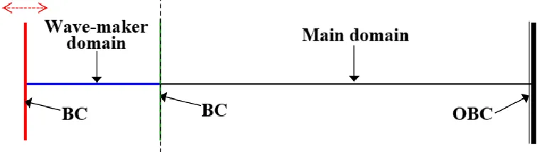
In order to numerically experiment with the OBCs for various situations, it is necessary to generate various types of information passing through the boundary of interest. For this, a piston type paddle of the type proposed in [12] was used. In the wave-maker domain, 4th_{order Runge-Kutta scheme and 4}th

order centred finite difference method are implemented for time and space, respectively, after mapping the movable domain that contracts and expands with time to the fixed domain. (See [12] for more details).

Figure 1: Schematic diagram of numerical experiments

Test cases Amplitude frequency Water depth Singular wave on shallow region 0.01 1.2566 5

Singular wave on deep region 1 3.7699 5

Long wave 4 0.1257 5

Discontinuity wave - - 0.3

(6)

3.3 Results

3.3.1 Validation of Numerical Model

Figure 2 shows the result of validation of the numerical solver. Both a moving discontinuity and a steady-state discontinuity are well captured (Figures 2.a. and b., respectively). In the case of still water (Figure 2.c), unwanted fluxes due to the topography are not observed since the equations are well balanced. Such an error occurs when solving with the form of equation (1).

Figure 2: Model validation with Toro’s cases [7]

3.3.2 Results of Numerical Tests

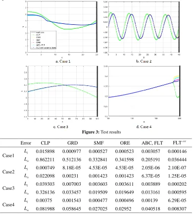
Figure 3 shows the results of the cases mentioned previously in Table 2. The thick black lines to the right of each domain in Figure3 indicate the OBC. In this experiment, all waves propagate from the left to the right.

CLP shows the largest error in all cases. The CLP produces the results very differently from the exact solution and generates even the phase shifts. It is very evident that information at the boundary is not radiated well but reflected back into the internal domain. Other boundary conditions work well when the solution is smooth. However, when the solutions have the discontinuities (case 4), the performances of each OBC are remarkablely different from each other. In this case, the FLT with the external data (FLText) shows more accurate results than ORE, SMF, and ABC. This implies that the OBC designed by the characteristic based method is superior in treating the discontinuities. In addition, as it can be seen through a comparison of FLT and FLText, using external data can yield much more accurate values.

(7)

larger In general, ORE and SMF show the similar results since the simulations have been performed when the slope of water level is not large. In general, errors tend to be less as the amplitude and frequency of the waves are smaller. In particular, if there is a discontinuity at the boundary, relatively larger errors occur.

Figure 3: Test results

4 Summary and Conclusions

The characteristics exist as many as the number of independent hyperbolic terms in the partial differential equations (PDEs). In the case of governing equation (1), there are two independent characteristics. Each characteristic information propagates through a unique path, which is called as the

Error CLP GRD SMF ORE ABC, FLT FLText

Case1 L1 0.015898 0.000977 0.000527 0.000523 0.003057 0.000146

L_ 0.862211 0.512136 0.332841 0.341598 0.205191 0.036444

Case2 L1 0.000749 8.18E-05 4.53E-05 4.53E-05 2.05E-06 2.10E-07

L_ 0.022098 0.00231 0.001423 0.001423 6.37E-05 1.25E-05

Case3 L1 0.039303 0.007003 0.003603 0.003611 0.003889 0.000202

L 0.326136 0.033457 0.019509 0.019649 0.013161 0.000595

Case4 L1 0.00375 0.001543 0.000477 0.000496 0.00139 6.29E-05

L 0.081988 0.058645 0.027025 0.02952 0.040518 0.008307

(8)

boundaries to the out of the domain, those characteristics at boundaries should be consistent with that of the governing equation. In other words, when a system is hyperbolic, boundary conditions must be consistent with those characteristics of the governing equations. In this respect, FLT and ABS show relatively better results because those solutions are the characteristics based OBCs, which were derived with the Riemann invariants preserving along the characteristic curve. Except for those two OBCs, the others are not based on the characteristic method, and the information passing through the boundary to the out of domain is primitively conserved. In [4], FLT is classified into the same group with SMF and ORE in that these OBCs show the hyperbolic phenomenon radiating information. Unlike FLT, however, SMF and ORE propagate the primitive variables rather than Riemann invariants. Therefore, errors occur due to the characteristic difference between the governing equations and the formulation of the boundary condition contaminating the inner domain. Meanwhile, when receiving information or external data from the outside of domain through the OBC, the characteristics are required to be defined according to the form of Riemann invariants, which is consistent and generates less error. Therefore, when some information propagates with the highly hyperbolic nature of the governing equations, such as the shallow water equation, it is strongly recommended to use a characteristic based OBC according to the results of this study.

Acknowledgements

This research was a part of the project titled “Development of integrated estuarine management system”, funded by the Ministry of Oceans and Fisheries, Korea and the National Research Foundation of Korea (NRF) Grant (No. 2017R1A2B4007977) funded by MSIP of Korea.

References

[1] B. Engquist, A. Majda, Absorbing boundary conditions for numerical simulation of waves. Proceedings of the National Academy of Sciences 74.5 (1977): 1765-1766.

[2] B. Gustafsson, High order difference methods for time dependent PDE. Vol. 38. Springer Science & Business Media, 2007.

[3] D. Givoli, Non-reflecting boundary conditions. Journal of compuational physics 94.1 (1991), 1-29. [4] E. Blayo, L. Debreu, Revisiting open boundary conditions from the point of view of characteristic

variables. Ocean modelling 9.3 (2005) 231-252.

[5] E. F. Toro, Riemann solvers and numerical methods for fluid dynamics: a practical introduction. Springer Science & Business Media, 2013, pp.315-336.

[6] E. F. Toro, Riemann solvers and numerical methods for fluid dynamics: a practical introduction. Springer Science & Business Media, 2013, pp.504-511.

[7] E. F. Toro, Shock-capturing methods for free-surface shallow flows. Wiley and Sons Ltd., 2001. [8] H. O. Kreiss and J. Lorenz. Initial-boundary value problems and the Navier-Stokes equations. Vol.

47. Siam, 1989.

[9] I. Orlanski, A simple boundary condition for unbounded hyperbolic flows. Journal of computational physics 21.3 (1976): 251-269.

[10] J. Oliger, A. Sundström. Theoretical and practical aspects of some initial boundary value problems in fluid dynamics. SIAM Journal on Applied Mathematics 35.3 (1978): 419-446.

(9)

[12] J. Orszaghova, A. G. Borthwick, and P. H. Taylor, From the paddle to the beach–A Boussinesq shallow water numerical wave tank based on Madsen and Sørensen’s equations. Journal of Computational Physics 231.2 (2012) 328-344.

[13] L. P. Røed, C. K. Cooper. A study of various open boundary conditions for wind-forced barotropic numerical ocean models. Elsevier oceanography series. Vol. 45. Elsevier, 1987. 305-335.

[14] Q. Liang, A. G. Borthwick. Adaptive quadtree simulation of shallow flows with wet-dry fronts over complex topography. Computers & Fluids 38.2 (2009) 221-234.

[15] R. G. Dean, R. A. Dalrymple, Water wave mechanics for engineers and scientists (Vol. 2). world scientific publishing Co Inc. 1991, pp.296-305.

[16] S.V. Tsynkov, Numerical solution of problems on unbounded domains. A review. Applied Numerical Mathematics27.4 (1998): 465-532.

[17] S. Ghader, J. Nordström. Revisiting well-posed boundary conditions for the shallow water equations. Dynamics of Atmospheres and Oceans 66 (2014): 1-9.