[Maina* 4(12): December, 2017] ISSN 2349-4506
Impact Factor: 2.785
G
lobal
J
ournal of
E
ngineering
S
cience and
R
esearch
M
anagement
DEVELOPMENT AND APPLICATION OF CRASH MODIFICATION FACTORS
FOR TRAFFIC FLOW PARAMETERS ON URBAN FREEWAY SEGMENTS
Eugene Vida Maina, Ph.D*, Janice R. Daniel, Ph.D
*Operations Systems Research Analyst, Dallas Fort Worth International Airport DFW Airport, TX 75261
Associate Professor Department of Civil and Environmental Engineering New Jersey Institute of Technology Newark, NJ 07102
DOI: 10.5281/zenodo.1119563
KEYWORDS
: Empirical Bayes (EB) Model, Safety Performance Functions (SPFs), Development of Crash
Modification Factors, (CMFs).ABSTRACT
Attempts to apply more evidence-based methodologies to traffic safety have recently intensified. One such attempt is the Highway Safety Manual (HSM, 2010), which provides crash modification factors (CMFs) for a variety of roadway treatments. CMFs provide traffic practitioners with the resources to estimate the safety effects of various countermeasures. At the moment, the HSM does not provide CMFs for traffic flow parameters despite the significant differences in the number of crashes on segments with similar geometric parameters and average annual daily traffic (AADT). This study develops CMFs associated with change in hourly traffic flow conditions for 2008 through 2011 on three similar urban freeway segments in New Jersey using Empirical Bayes (EB) for before-after road safety studies. Specifically, this study focuses on traffic density expressed as level of service (LOS). Results show significantly that, as the LOS deteriorates from A to B, B to C, C to D, and D to E, the resultant CMFs are 0.673, 1.11, 0.865, and 1.452 respectively. This demonstrates that traffic flow parameters have some significant effect on roadway safety, therefore needs to be investigated further and eventually included in the future editions of the HSM.
INTRODUCTION
Although many safety studies have addressed how geometric parameters influence roadway safety, few have investigated and acknowledged that traffic flow parameters have significant influence on safety. One such study is by Kononov et al. (2008) which states that transportation practitioners usually believe that additional capacity due to additional lanes is associated with increased safety. However, how much safety and for what time period is generally not considered.
A misinterpretation of the real relationship between accidents and exposure usually leads analysts to simply divide the number of accidents by volume of vehicles at a given site (Nordback et al., 2014), a metric Hauer (1995) states that represents a fundamental misunderstanding and the results can be misleading. To increase accuracy and certainty, through thorough research, in 2010, transportation practitioners were presented with a significant tool, the first edition of the HSM. Part D of the manual provides CMFs which serve to predict the safety effect for a variety of actions referred to as either countermeasures, interventions, treatments or decisions (HSM, 2010). Through continued research there are efforts to update the current CMFs and include new CMFs in the next edition of the HSM. One such effort is by the American Association of State Highway and Transportation Officials (AASHTO) in conjunction with Transportation Research Board (TRB) through anticipated project NCHRP 17-72 calling for the updating of current CMFs and inclusion of new CMFs for the next edition of the HSM. In an effort to improve roadway safety and the fact that roadway locations with similar geometric features and AADT have recorded significantly different number of accidents (Qin et al., 2000), this study evaluates traffic flow parameters and their effects on roadway safety by developing relative CMFs.
[Maina* 4(12): December, 2017] ISSN 2349-4506
Impact Factor: 2.785
G
lobal
J
ournal of
E
ngineering
S
cience and
R
esearch
M
anagement
road safety studies, such as those used for geometric parameters in the HSM and applies the method to accidents on basic freeway segments when the LOS deteriorates. To the knowledge of this paper’s authors, these are the first CMFs associated with LOS on basic freeway segments. Research by Kononov et al. (2008), Poch and Mannering (1996), and the calling for continued research in this area by TRB show such studies as needed, rendering this study as an important initial step towards fulfilling this need.Improved insight for the basic relationship of traffic flow parameters and how they influence safety on roadways will assist to lay the foundation for future studies and allow transportation safety researchers to investigate specific geometric, traffic flow, human or weather factors that may influence safety on roadways. The motivation for this study is not to establish conclusive CMFs for changing LOS, but to lay a foundation for future studies in this area and open up discussion on how traffic flow parameters influence roadway safety. This study achieves this by presenting a case study where on the same and similar freeway segments, the number of accidents/incidences are measured and evaluated when the LOS deteriorates progressively from A to E.
LITERATURE REVIEW
The HSM presents many CMFs for geometric parameters for both interrupted and uninterrupted facilities. They show the relationship(s) between the number of accidents and given roadway parameters established using crash data from hundreds of locations with comparable roadway features (Nordback et al., 2014). The HSM shows how to predict crashes at similar basic freeway segments by using safety performance functions (SPFs) and predictable models such as EB to determine CMFs based on geometric parameters and AADT. The manual however does not consider other factors like traffic flow/operational parameters which although not quantified, studies acknowledge that they do influence safety (Kononov et al., 2011; 2012a; 2012b; 2012c).
However conflicting or consistent the conclusions of previous studies, they all show that there is a relationship between the number of accidents and traffic flow parameters such as hourly volumes, although its precise form is still unknown (Qin et al., 2000). Logically, accidents at a specific time should relate closely to the hourly traffic volumes or more accurately, to real-time traffic volumes. Qin et al. (2000) and Abdel-Aty and Pande (2007) continue on that the exposure measures such as AADT, Vehicles-Miles Travelled (VMT), or Number of Vehicles Entering (NEV), are applied to quantify the opportunity for accidents and are aggregate quantities that do not consider temporal traffic variation experienced though the day. In their study’s literature review, Abdel-Aty and Pande (2007) sites Frantzeskakis and Iordanis (1987); Persaud & Nguyen (1998) and Abdel-Aty, Pemmanaboina, & Hsia, (2006) by stating that the mentioned ‘microscopic’ traffic parameters not only include hourly volume but logical measures of congestion represented by v/c ratio and LOS, along with distributional properties of variation in speed.
As stated, previous studies have found different results. For example, as cited by Frantzeskakis and Iordanis (1987), Lord et al. (2005) and Persaud and Nguyen (1998) show that both the number of accidents and crash rates increase as the LOS deteriorates from A to F. However, Cedar and Livneh, 1982a & 1982b, Qin et al. (2000) and Roess et al. (2011) show that the relationship between the number of accidents and the disaggregate exposure, i.e. hourly volume, is indeed non-linear. A trend Lord et al. (2005) also finds while investigating relationships between crashes and traffic flow characteristics in Quebec, Canada. Using predictive models, three series of predictive models that relate crash-flow, crash-flow-density and crash-flow-volume to capacity (v/c) ratio and determines that traffic volume, vehicle density, and the v/c ratio have direct influence on the likelihood and severity of a crash.
[Maina* 4(12): December, 2017] ISSN 2349-4506
Impact Factor: 2.785
G
lobal
J
ournal of
E
ngineering
S
cience and
R
esearch
M
anagement
using hierarchical Bayesian framework with Markov Chain Monte Carlo (MCMC) algorithms to estimate the posterior distributions for crash probabilities as a function of hourly volume and time of day, the study shows that the expected crash count on two equal length segments with the same AADT and physical characteristics will vary according to the distribution of traffic volume through the time of the day.Knowing that on a basic freeway segment, hourly volumes are dynamic and are constantly changing together with the fact that an accident is a rare, random, and independent event, appropriate predictive and SPFs statistical models are used by this study to account for either over-dispersion or under-dispersion and regression-to-mean (RTM) characteristics associated with crash data Tegge et al. (2010)and bias in site selection Lan et al. (2009). Studies show that the appropriate SPFs and predictive models to be Poisson regression distributions and negative binomial (NB) distributions (Anastasopoulos and Mannering, 2009; Lord and Mannering, 2010; Pande et al., 2000; Poch and Mannering, 1996;Stamatiadis et al., 2009) and the EB used to correct for the RTM effects (Gross et al., 2010; Hauer, 1995; Srinivasan et al., 2008).
MODELLING APPROACH
CMFs are developed by evaluating roadway incidences before and after implementation of a given countermeasure(s), and as stated in the FHWA’s Crash Modification Factor Clearinghouse, countermeasures can be positive (improve safety) or negative (degrade safety). As a result, it is paramount to conduct prior tests before implementation but most importantly, the selected method of evaluation should be fitting, inclusive and reliable. This study adopts the EB before-after model because it has the ability to account for (1) RTM effects due to sites experiencing randomly high short-term crash counts selected for treatment and show reduction in crashes afterwards when these counts regress towards their true long-term mean and vice versa, and (2) changes in traffic volumes, time trends in crash occurrence due to changes over time in factors like weather, human habits, and crash reporting practices (Gross et al., 2010; Persaud and Lyon, 2007) , and bias in site selection (Lan et al., 2009). In addition, in the past 30 years, EB models have been used successfully by other researchers to perform this type of evaluations (Elvik, 2008).
Empirical Bayes (EB) Model
In the EB before-after evaluation of a treatment effect, the change in crashes at a basic freeway segment is given by:
𝐴 − 𝐵 (1)
where B is the ‘expected’ number of accidents that would have occurred in the ‘after’ period without treatment and A is the number of accidents observed in the after period. These changes may be due to differences in traffic volumes, along with RTM, trends in crash reporting, and other factors, it is now accepted that the count of crashes before a treatment by itself is not a good estimate of B (Hauer, 1996 cited by Persaud and Lyon, 2007). Instead, B is estimated from an EB procedure in where SPFs are initially used to estimate the ‘predicted’ number of crashes expected in a given time ‘before’ period at selected locations with similar traffic volumes and physical characteristics to that being analyzed. The sum of these SPF ‘predicted’ estimates (PB) is then combined with the
observed accidents (OB) in the ‘before’ period to obtain the ‘expected’ number of accidents (EB) before treatment
also referred to as the unadjusted EB estimate. This estimate of EB is
𝐸𝐵= 𝑤. 𝑃𝐵+ (1 − 𝑤)
𝑂𝐵
𝑛 (2)
where n is the time period of observation and w is the weight factor estimated as
𝑤 = 1
[Maina* 4(12): December, 2017] ISSN 2349-4506
Impact Factor: 2.785
G
lobal
J
ournal of
E
ngineering
S
cience and
R
esearch
M
anagement
where k is the dispersion parameter of the NB distribution that is assumed for the crash counts used in estimating the SPF, and Pn is the predicted number of accidents for period time n. k is estimated from the SPF calibration
procedure with the use of maximum likelihood procedure.
Safety Performance Functions (SPFs)
As discussed, SPFs also referred to as predictive models Zhong et al. (2008) are part of the EB studies and are used to determine the ‘predicted’ accident counts. SPFs are regression statistical models relating accident counts to their causing factors. There are several SPFs but the two most accurate and common types are Poisson and NB models (Tegge et al., 2010).
This study develops SPFs for the hourly accident frequency on basic freeway segments, by estimating five different hourly accident frequencies for the ‘predicted’ accidents when the basic freeway segments at the study sites are operating at LOSs A, B, C, D, and E. LOS F was not evaluated since the segment is failing in this state, that is the demand flow exceeds capacity. For all LOSs, the dependent/outcome variable, hourly crash frequency, is a non-negative integer. Since accident data is discrete, nonnegative, and sporadic, the Poisson regression model is the natural first choice for modeling (Poch and Mannering, 1996). However, as discussed, the Poisson regression model has a key setback, that is the variance of the dependent variable is constrained to be nearly or equal to its mean. Literature shows that accident data is likely to be over-dispersed (Tegge et al., 2010)that is, the variance is likely to be significantly greater than the mean. In such a situation, if the Poisson is used in evaluation, the model coefficients tend to be underestimated and biased. To correct or account for such, the NB distribution is adopted.
The NB model is derived from the Poisson model. For the Poisson model, the chance of having a certain number of accidents at a given basic freeway segment i(yi) per hour (where yi is a non-negative integer) is
𝑃(𝑦𝑖) =𝑒𝑥𝑝(−𝜇𝑖)𝜇𝑖 𝑦𝑖
𝑦𝑖! (4)
where P(yi) is the probability of an accident occurring on segment i, ni times per hour; and µi is the Poisson
parameter for segment i, which is equal to segment i’s probable accident frequency per hour. The accident data is fit to the Poisson model by specifying the Poisson parameter µi to be a function of explicatory roadway and traffic
variables of traffic volume, posted speed limit, number of lanes, lane width, shoulder width and density. This is accomplished by specifying the Poisson parameters as
ln 𝜇𝑖= 𝛽𝑋𝑖 (5)
where Xi is a vector of explicatory variables; and β is a vector of estimable coefficients. The Poisson model defined
in equations 4 and 5 is estimable by standard maximum likelihood methods with the likelihood function
𝐿(𝛽) = Π𝑖𝑒𝑥𝑝[−𝑒𝑥𝑝(𝛽𝑋𝑖)][𝑒𝑥𝑝(𝛽𝑋𝑖)]
𝑦𝑖
𝑦𝑖! (6)
Through integration, equation 6 gives the unconditional distribution of yi. The formulation of this distribution is
[Maina* 4(12): December, 2017] ISSN 2349-4506
Impact Factor: 2.785
G
lobal
J
ournal of
E
ngineering
S
cience and
R
esearch
M
anagement
𝑃(𝑦𝑖) =Γ (𝑦𝑖+ 1 𝑘) 𝑦𝑖! Γ (1𝑘)
( 𝑘𝜇𝑖 1 + 𝑘𝜇𝑖)
𝑦𝑖
( 1
1 + 𝑘𝜇𝑖)
1 𝑘
(7)
where Γ is the gamma function, μ is the negative binomial mean, and k is the dispersion parameter. The NB model allows the mean to differ from the variance such that
var 𝑛𝑖= 𝐸(𝑛𝑖)[1 + 𝛼𝐸(𝑛𝑖)] (8)
where α is the measure of the dispersion and can be estimated using the standard maximum likelihood techniques. The appropriateness of the NB relative to the Poisson model is determined by the statistical significance of the estimated α. If α is not statistically different from zero, the NB simply reduces to Poisson regression with var 𝑛𝑖= 𝐸(𝑛𝑖). If α significantly different from zero, then the NB is adopted and the Poisson regression is inappropriate.
The log linear model for the ith roadway segment with q parameters X
i1, Xi2, Xi3 ... Xiq, and regression coefficients
β0, β1 … βq takes on the form
log(𝜇) = 𝛽0+ 𝛽1𝑋𝑖1+ 𝛽2𝑋𝑖2+ ⋯ + 𝛽𝑞𝑋𝑖𝑞 (9)
Using equation 9, the ‘predicted’ number of accidents are estimated and together with the observed accidents used to calculate EB as shown in equation 2. The final and main task is to develop the CMFs relative to the deteriorating
LOS conditions discussed.
Development of Crash Modification Factors, (CMFs)
The ‘expected’ accident frequency found in equation 2 is used in the development of CMFs as published by the U.S. Department of Transportation Federal Highway Administration’s “A Guide to Developing Quality Crash Modification Factors” (Gross et al., 2010). In the initial step, the ‘expected’ accident frequency in the ‘after’ period in the treatment group that would have occurred without treatment, (EA) is
𝐸𝐴= 𝐸𝐵∗ (
𝑃𝐴
𝑃𝐵) (10)
where EB, and PB are as previously described and PA, is the predicted number of crashes, (i.e. sum of SPF
estimates) in the ‘after’ period. The variance of EA is estimated as
𝑣𝑎𝑟 (𝐸𝐴) = 𝐸𝐴∗ (
𝑃𝐴 𝑃𝐵
) ∗ (1 − 𝑤)
(11)
and finally, the CMF is approximately equal to the ‘after’ period accident counts divided by the EA. It is an
[Maina* 4(12): December, 2017] ISSN 2349-4506
Impact Factor: 2.785
G
lobal
J
ournal of
E
ngineering
S
cience and
R
esearch
M
anagement
𝐶𝑀𝐹 =
(𝑂𝐴
𝐸𝐴)
1 + (𝑣𝑎𝑟(𝐸𝐴)
𝐸𝐴2 ) (12)
𝑣𝑎𝑟𝐶𝑀𝐹= 𝐶𝑀𝐹2[
((1 𝑂⁄ 𝐴) + (𝑣𝑎𝑟𝐸𝐴⁄𝐸𝐴2))
(1 + (𝑣𝑎𝑟𝐸𝐴⁄𝐸𝐴2))2 ]
(13)
DATA COLLECTION, DESCRIPTION AND PREPARATION
The data for this study were collected from New Jersey Department of Transportation’s straight-line, accident and traffic counts databases. Hourly traffic volumes were matched with the accident and geometric features for each of the freeway segments to ensure consistency. Entities that had missing information were eliminated and consequently not used for evaluation. The study period runs from 2008 through 2011 and a total 14 one mile long basic freeway segments are studied. The count stations at these locations provide 24-hour traffic volume, resulting in 96 hours of volume counts a day and 1344 hours for the entire period of study.
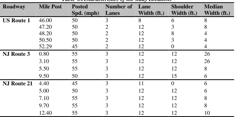
As Table 4.1 shows, three urban freeways are considered for evaluation; five segments on US 1 and NJ 21 and four segments were selected on NJ 3. Characteristics for each freeway segment are summarized; they are posted speed (mi/hr.), number of lanes, lane width (ft.), shoulder width (ft.), and median width (ft.).
Table 4.1Characteristics of the study Locations
Roadway Mile Post Posted Spd. (mph)
Number of Lanes
Lane Width (ft.)
Shoulder Width (ft.)
Median Width (ft.) US Route 1 46.00 50 3 8 6 8
47.20 50 2 12 3 8
48.20 50 2 12 8 4
50.50 50 2 12 3 4
52.29 45 2 12 0 4
NJ Route 3 0.80 55 3 12 12 26
3.10 55 3 12 12 26
5.50 55 3 12 12 8
9.50 50 3 12 15 6
NJ Route 21 4.40 45 3 11 0 6
5.00 50 3 12 12 6
7.10 55 3 12 12 8
9.70 55 3 12 12 8
12.40 55 3 12 12 10
The volume densities for each hour were calculated and respective LOS assigned for each of the 1344 entries using the procedures presented in the Highway Capacity Manual (2010). The data were then sorted according to their LOS and the entities with the LOS F were not considered for evaluation as discussed. There were 177 entities that corresponded with LOS F. As a result, the sample size reduced from 1344 to 1167 hours.
[Maina* 4(12): December, 2017] ISSN 2349-4506
Impact Factor: 2.785
G
lobal
J
ournal of
E
ngineering
S
cience and
R
esearch
M
anagement
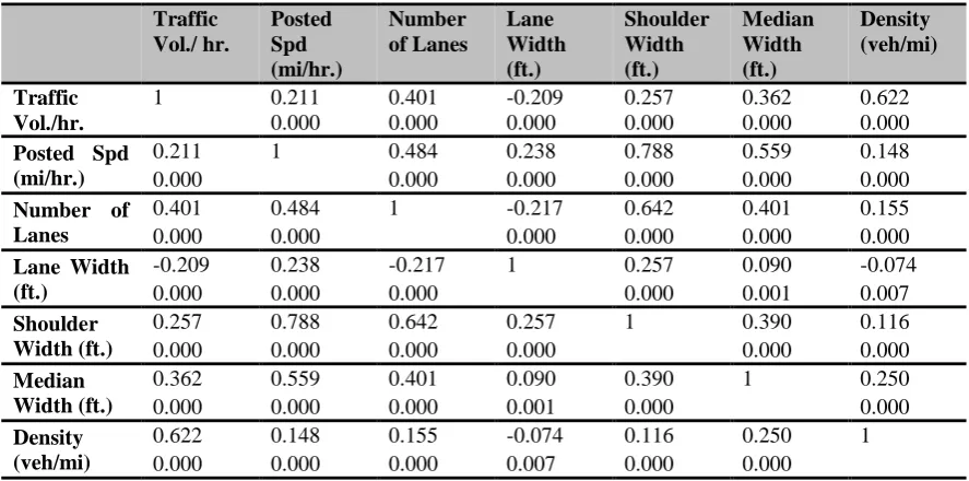
which in return makes some variables to be statistically insignificant while they are actually significant and vice versa. For example, the F-Test may show that the data fits well even though none of the predictor variables influences the dependent variable significantly (Kutner et al., 2004). The results of the correlation test are presented in Table 4.2.Table 4.2Pearson Correlation Matrix
Traffic Vol./ hr. Posted Spd (mi/hr.) Number of Lanes Lane Width (ft.) Shoulder Width (ft.) Median Width (ft.) Density (veh/mi) Traffic Vol./hr.
1 0.211 0.401 -0.209 0.257 0.362 0.622
0.000 0.000 0.000 0.000 0.000 0.000
Posted Spd (mi/hr.)
0.211 1 0.484 0.238 0.788 0.559 0.148
0.000 0.000 0.000 0.000 0.000 0.000
Number of Lanes
0.401 0.484 1 -0.217 0.642 0.401 0.155
0.000 0.000 0.000 0.000 0.000 0.000
Lane Width (ft.)
-0.209 0.238 -0.217 1 0.257 0.090 -0.074
0.000 0.000 0.000 0.000 0.001 0.007
Shoulder Width (ft.)
0.257 0.788 0.642 0.257 1 0.390 0.116
0.000 0.000 0.000 0.000 0.000 0.000
Median Width (ft.)
0.362 0.559 0.401 0.090 0.390 1 0.250
0.000 0.000 0.000 0.001 0.000 0.000
Density (veh/mi)
0.622 0.148 0.155 -0.074 0.116 0.250 1 0.000 0.000 0.000 0.007 0.000 0.000
Following the outcome of the correlation test, the model(s) with the best fitting predictor variables were selected on the criteria that: (1) the predictor variables had to show no or have weak correlation (that is the r value had to be between the absolute value of 0 and 0.29 (Navidi, 2008), (2) the predictor variables have to be statistically significant at a 0.1 significance level, and (3) the selected model(s) had to have traffic volume and density among the predictor variables. Three models met the prescribed criteria:
Model I: Traffic Volume, Posted Speed, Lane Width, Density;
Model II: Traffic Volume, Shoulder Width, Lane Width, Density; and
Model III: Traffic Volume, Posted speed, Lane Width, Number of Lanes, Shoulder Width, Density
DATA ANALYSIS AND INTERPRETATION
The first step in this section involved testing each model to determine which model’s data fit well. To do so, a goodness-of-fit test was conducted and the results were presented in Table 4.3 as follows
Table 5.1Goodness-of-Fit test for Models I, II, and III
MODEL I MODEL II MODEL III
LOS Parameter Value df Value/df Value df Value/df Value df Value/df
A
Deviance 463.37 432 1.07 464.32 432 1.08 461.90 429 1.08
Pearson
Chi-Square 458.56 432 1.06 463.55 432 1.07 452.82 429 1.06
Sig. 0.00 0.00 0.00
B
Deviance 268.98 245 1.10 268.06 245 1.09 269.49 242 1.11
Pearson
Chi-Square 276.64 245 1.13 271.74 245 1.11 267.48 242 1.11
Sig. 0.00 0.00 0.00
[Maina* 4(12): December, 2017] ISSN 2349-4506
Impact Factor: 2.785
G
lobal
J
ournal of
E
ngineering
S
cience and
R
esearch
M
anagement
PearsonChi-Square 259.21 261 0.99 274.25 261 1.05 260.49 258 1.01
Sig. 0.00 0.00 0.00
D
Deviance 119.68 99 1.21 119.63 99 1.21 119.79 96 1.25
Pearson
Chi-Square 100.92 99 1.02 100.25 99 1.01 101.87 96 1.06 Sig. 0.29 0.14 0.01
E
Deviance 108.71 100 1.09 109.82 100 1.10 100.93 97 1.04
Pearson
Chi-Square 101.09 100 1.01 108.78 100 1.09 90.42 97 0.93 Sig. 0.00 0.00 0.00
At each LOS for all the three models, Table 5.1 shows the respective Deviances and Pearson Chi-Squares values and their respective significance levels. The Deviance has an approximate chi-square distribution with n-p degrees of freedom, df, where n is the number of observations and p is the number of the predictor variables including the intercept. It is expected that the value of the chi-square random variable to be equal to the df, that is this ratio is expected to be equal or approximately equal to 1. Using this criterion and referring to the values in Table 5.1, all the three models fit the data well since the ratios of the Deviance to df (Value/df) are approximately 1 at a significance level of 0.1.
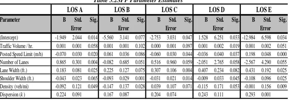
However, only model III was considered for the development of the SPFs because it contains more variables than models I and II. The values of the SPF evaluations, are presented in Table 5.2 as follows
Table 5.2SPF Parameter Estimates
Table 5.2 shows the NB regression coefficients for each predictor variable and k at each LOS, along with their standard errors, and significance levels. Since all the ks are greater than zero, it is an indication that the variances are greater than the means, a phenomena referred to as over-dispersion and therefore the NB distribution is appropriate.
The results show that at all LOSs the lane width is positive indicating that crash frequency increased with increased lane width. The posted speed is positive at LOS B, and E, and negative at LOS A, C, and D indicating differing effects by LOS of posted speed on crash frequency. The number of lanes is positive at all LOS except at LOS C and A, indicating that for LOS B, D, and E, crash frequency increased as the number of lanes increased. The shoulder width has a negative influence on crash frequency indicating that the crash frequency decreased as the shoulder width increased. Density is negative at all LOSs except at LOS C an indication that crash frequencies decreased as density increased.
Parameter B Std. Error
Sig. B Std. Error
Sig. B Std. Error
Sig. B Std. Error
Sig. B Std. Error
Sig.
(Intercept) -1.949 2.044 0.014 -5.560 3.141 0.077 -2.753 3.031 0.047 1.528 6.251 0.033 -12.984 6.598 0.034 Traffic Volume / hr. 0.001 0.001 0.058 0.001 0.001 0.102 0.000 0.001 0.097 0.001 0.002 0.019 0.001 0.002 0.051 Posted Speed Limit (m/h) -0.070 0.030 0.020 0.061 0.036 0.086 -0.060 0.030 0.044 -0.036 0.040 0.037 0.198 0.048 0.000 Number of Lanes 0.865 0.301 0.004 -0.082 0.685 0.051 0.516 0.960 0.059 -2.051 2.765 0.058 -2.567 4.290 0.055 Lane Width (ft.) 0.183 0.081 0.025 0.225 0.127 0.075 0.307 0.106 0.004 0.407 0.234 0.082 0.431 0.192 0.025 Shoulder Width (ft.) -0.043 0.023 0.065 -0.093 0.029 0.001 -0.031 0.021 0.014 -0.009 0.033 0.045 -0.108 0.096 0.025 Density (veh/mi) -0.092 0.121 0.049 -0.147 0.137 0.028 0.039 0.107 0.071 -0.115 0.171 0.053 -0.001 0.156 0.009
Dispersion (k) 0.224 0.091 0.167 0.087 0.204 0.074 0.243 0.111 0.293 0.001
[Maina* 4(12): December, 2017] ISSN 2349-4506
Impact Factor: 2.785
G
lobal
J
ournal of
E
ngineering
S
cience and
R
esearch
M
anagement
As discussed in Section 3, the SPF coefficients are used to estimate the ‘predicted’ numbers of accidents, the dispersion values found during the SPF development are used to estimate the weight factors and the ‘expected’ number of accidents. Along with the observed/actual number of accidents, the results of this task are presented in Table 5.3 as follows
Table 5.3Actual, Predicted and Expected Number of Accidents
LOS
Observed / Actual Accidents
SPF ‘Predicted’ Accidents
Weight factor
EB ‘Expected’ Accidents
A 408 174.811 0.025 402.193
B 297 191.368 0.030 293.795
C 434 253.915 0.019 430.589
D 212 144.177 0.028 210.118
E 267 125.582 0.026 263.258
The values presented in Table 5.3, establish the before-after conditions for all LOSs and therefore give all the information required to calculate the EA for deterioration in LOS. For example, when the LOS changes from A to
B, the OB is 408, the OA is 297, the PB is 174.81, the PA is 191.37, and EB is 402.19. Using these values and the
procedure discussed in Section 3.3, EA for all the LOS changes were calculated and presented in Table 5.4 as
follows
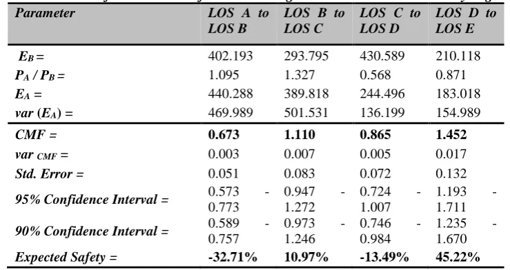
Table 5.4Crash Modification Factors for deteriorating LOS on Basic Urban Freeway Segments
Parameter LOS A to
LOS B
LOS B to LOS C
LOS C to LOS D
LOS D to LOS E
EB = 402.193 293.795 430.589 210.118
PA / PB = 1.095 1.327 0.568 0.871
EA = 440.288 389.818 244.496 183.018
var (EA) = 469.989 501.531 136.199 154.989
CMF = 0.673 1.110 0.865 1.452
var CMF = 0.003 0.007 0.005 0.017
Std. Error = 0.051 0.083 0.072 0.132
95% Confidence Interval = 0.573 -
0.773
0.947 - 1.272
0.724 - 1.007
1.193 - 1.711
90% Confidence Interval = 0.589 -
0.757
0.973 - 1.246
0.746 - 0.984
1.235 - 1.670
Expected Safety = -32.71% 10.97% -13.49% 45.22%
Along with the EB, for each deterioration in LOS, Table 5.4 also presents the ‘after’ period SPF estimates to the
‘before’ period SPF estimates (𝑃𝐴⁄𝑃𝐵) ratios, EAs and their respective variances. These values were used to
estimate the respective CMFs also presented in Table 5.4. A less than one CMF value shows improvement in safety, a one CMF value shows no effect on safety, and a larger than one value shows degradation in safety. Using this argument and referring to CMFs in Table 5.4, LOS B and LOS D are the safest since their resultant CMFs are less than one and LOS C and LOS E are hazardous since their resultant CMFs are more than one.
[Maina* 4(12): December, 2017] ISSN 2349-4506
Impact Factor: 2.785
G
lobal
J
ournal of
E
ngineering
S
cience and
R
esearch
M
anagement
which is less than 1.0. Thus, at 90% confidence level it can be interpreted that the numbers of accidents will reduce by 33% when the LOS deteriorates from A to B and by 14% when LOS deteriorates from LOS C to D. Also, at 90% confidence level, the numbers of accidents are expected to increase by 11% when the LOS deteriorates from LOS B to C and by 45% when the LOS deteriorates from D to E. More observations are required to detect the same of with 95 % certainty for all LOSs.CONCLUSION
The analysis performed show the potential for traffic flow parameters SPFs to be estimated for the inclusion in the future versions of the HSM. It also opens up the discussion for the creations for CMFs so that future investigations can contribute to better understand and quantify the effects traffic flow parameters have on roadway safety. The main objective for this study was not to estimate definitive CMFs for changes in LOS on basic freeway segments, but to rather show that there is a need, it can be done and how to do it. As a result, this study instigates the discussion of what a traffic flow parameter SPF and CMF is and why they are important by presenting a case study from fourteen sites with 1167 hours of observations.
The CMFs calculated in this study show that: (1) traffic flow parameters in this case hourly volumes have significant influence on urban freeway safety; (2) the relationship between hourly traffic volume and numbers of accidents can be quantified; finally, the relationship between hourly traffic volumes and the numbers of accidents is sinusoidal with LOSs B and D being the safest and LOSs C and E being hazardous.
Results show that, LOS B is the safest of all the five measures of effectiveness, this could be attributed the fact that at this LOS, the drivers begin to respond to the existence of other vehicles in the traffic stream even though traffic flow is still at free-flow speed. Although drivers can still easily maneuver within the traffic stream, they become more vigilant in searching for gaps in the lane flows. LOS E is the most hazardous, the degradation safety could be attributed to the fact that there is few of no usable gaps in the traffic stream, and any trepidation due to lane changing or merging maneuvers create shock waves and queuing in the traffic stream as a result creating conducive conditions for incidences.
The models presented are specific, have been used and tested before, and are appropriate to be used elsewhere. While the findings of this study may not apply on other transportation facilities, the same procedure can be applied. However, the sample size should be increased to find more accurate and appropriate results. This study provides the first traffic flow parameter SPFs and CMFs, however, more research is needed to precisely understand the effects of traffic flow parameters on roadway safety. As technology for counting vehicles and recording traffic incidences becomes more familiar and improved, appropriate CMFs should be created. As a result, this may lead to potential inclusion of traffic flow SPFs and CMFs in future HSM editions.
Improved knowledge on this topic could lead to efficient traffic planning and control of present and future transportation facilities hence improving safety. In addition, this could lead to (1) better understanding of what facilities and conditions that are safer for drivers, (2) identification of other variables that might influence roadway safety such as road surface condition, human and weather features, and (3) better understanding of the already identified variables. Thus, continuing to design and maintaining safer transportation facilities.
REFERENCES
1. Abdel-Aty, M. and A. Pande, 2007. Crash Data Analysis: Collective vs. Individual Crash Level Approach. Journal of Safety Research, Vol. 38, 581-587.
2. American Association of State Highway and Transportation Officials, 2010. Highway Safety Manual, 1st ed. AASHTO, Washington, DC.
3. Anastasopoulos, P. C. and F. L. Mannering, 2009. A note on Modelling Vehicle Accident Frequencies with Random-Parameters Count Models. Accident Analysis & Prevention, Vol. 41, 154-159.
4. Cedar A., and M. Livneh, 1982a. Relationship between Road Accidents and Hourly Traffic Flow-I. Accident Analysis & Prevention, No. 1, Vol. 14, 19-44.
[Maina* 4(12): December, 2017] ISSN 2349-4506
Impact Factor: 2.785
G
lobal
J
ournal of
E
ngineering
S
cience and
R
esearch
M
anagement
6. Elvik, R., 2008. The predictive validity of empirical Bayes estimates of road safety. Accident Analysisand Prevention 40, 1964–1969.
7. Frantzeskakis, J., and Iordanis, D., 1987. Volume to capacity ratio and traffic accidents on interurban four-Lane highways in Greece. Transportation Research Record, 1112, 29−38.
8. Gross, F., Persaud, B. and C. Lyon, 2010. A Guide to Developing Quality Crash Modification Factors. FHWA-SA-10-032.
9. Hauer, E., 1995. On exposure and accident rate. Traffic Engineering & Control 36 (3), 134-138. 10. Hauer, E., 1996. Statistical Test of the Difference between Expected Crash Frequencies. Transportation
Research Record, No. 1542, 24-39.
11. Kononov, J., Bailey, B., and B. K. Allery, 2008. Relationships between Safety and Both Congestion and Number of Lanes on Urban Freeways. Transportation Research Record, No. 2083, 26-39.
12. Kononov, J., Hersey S., Reeves D., and B. K. Allery, 2012a. Relationship between Freeway Flow Parameters and Safety and Its Implications for Hard Shoulder Running. Transportation Research Record, No. 2280, 10-17.
13. Kononov, J., Hersey S., Reeves D., and B. K. Allery, 2012b. Relationship between Traffic Density, Speed, and Safety and Its Implications for Setting Variable Speed Limits on Freeways. Transportation Research Record, No. 2280, 1-9.
14. Kononov, J., Lyon, C. and B. K. Allery, 2011. Relation of Flow, Speed, and Density of Urban Freeways to Functional Form of a Safety Performance Function. Transportation Research Record, No. 2236, 11-19.
15. Kononov, J., Reeves, D., Durso, C., and B. K. Allery, 2012c. Relationship between Freeway Flow Parameters and Safety and Its Implication for Adding Lanes. Transportation Research Record, No. 2279, 118-123.
16. Kutner, M. H., Nachtsheim, C. J. and J. Neter, 2004. Applied Linear Regression Models. 4th Edition.
McGraw Hill Companies.
17. Lan, B., Persaud, B., Lyon C. and R. Bhim, 2009. Validation of a Full Bayes Methodology for Observational Before-After Road Safety Studies and Application to Evaluation of Rural Signal Conversions. Accident Analysis & Prevention, Vol. 41, 574-580.
18. Lord D. and F. Mannering, 2010. The statistical analysis of crash-frequency data: A review and assessment of methodological alternatives. Accident Analysis and Prevention, Part A Vol. 44, 291-305. 19. Lord, D., A. Manar, and A. Vizioli, 2005. Modeling Crash-Flow-Density and Crash-Flow-V/C Ratio Relationships for Rural and Urban Freeway Segments. Accident Analysis & Prevention, No. 1, Vol. 37, 185-199.
20. Navidi, W., 2008. Statistics for Engineers and Scientists. 2nd Edition. McGraw Hill Companies.
21. Nordback, K., Marshall, W. E., and B. N. Janson, 2014. Bicyclist safety performance functions for a U.S. city. Accident Analysis& Prevention 65, 114-122.
22. Pande, A., Abdel-Aty M. and A. Das, 2000. A Classification Tree Based Modeling Approach for Segment Related Crashes on Multilane Highways. Accident Analysis and Prevention. Vol. 38 391-398. 23. Persaud, B., and C. Lyon, 2007. Empirical Bayes before–after studies: lessons learned from two decades
of experience and future directions. Accident Analysis and Prevention 39, 546–555.
24. Persaud, B., and Nguyen, T., 1998. Disaggregate safety performance models for signalized intersections on Ontario provincial roads. Transportation Research Record, 1635, 113−120.
25. Persaud, Bhagwant N., and Mucsi, K., 1995. Microscopic accident potential models for two-lane rural roads. Transportation Research Record, No. 1485, 134-139.
26. Poch, M. and F. Mannering, 1996. Negative Binomial Analysis of Intersection – Accident Frequencies. Journal of Transportation Engineering. Vol. 122, No.2.
27. Qin, X., Ivan, J. N., Ravishanker, N., Liu, J. and D. Tepas, 2000. Bayesian Estimation of Hourly Exposure Functions by Crash Type and Time of Day. Accident Analysis and Prevention, Vol. 38, No. 5, 1071-1080.
28. Roess, R. P., Prassas E. S., and W. R. McShane, 2011. Traffic Engineering. Pearson Prentice Hall Inc.
[Maina* 4(12): December, 2017] ISSN 2349-4506
Impact Factor: 2.785
G
lobal
J
ournal of
E
ngineering
S
cience and
R
esearch
M
anagement
30. Stamatiadis, N., Pigman, J., Sacksteder, J., Ruff, W. and D. Lord, 2009. Impact of Shoulder Width andMedian Width on Safety. NCHRP Report 633.
31. Tegge, R. A., Jo, J. and Y. Ouyang, 2010. Development and Application of Safety Performance Functions for Illinois. Research Report ICT-10-066. Illinois Department of Transportation.