Volume 41 - Article 31 | Pages 913–948

(1)

VOLUME 41, ARTICLE 31, PAGES 913

-

948 PUBLISHED 9 OCTOBER 2019

https://www.demographic-research.org/Volumes/Vol41/31/ DOI: 10.4054/DemRes.2019.41.31

Research Article

A spatial dynamic panel approach to modelling

the space-time dynamics of interprovincial

migration flows in China

Yingxia Pu

Xinyi Zhao

Guangqing Chi

Jin Zhao

Fanhua Kong

This open-access work is published under the terms of the Creative Commons Attribution 3.0 Germany (CC BY 3.0 DE), which permits use, reproduction, and distribution in any medium, provided the original author(s) and source are given credit.

(2)

1 Introduction 914

2 Literature review 916

3 Methods 919

3.1 General dynamic panel data model 919

3.2 Spatial dynamic panel data model 921

3.3 Interpreting the space-time effects of migration processes 923

4 Results 925

4.1 Model parameter estimates 927

4.2 Analysis of space-time effects 930

4.2.1 Population size 933

4.2.2 GDP 934

4.2.3 Age structure 935

4.2.4 Real wages 936

5 Conclusions 937

6 Acknowledgements 938

References 939

(3)

A spatial dynamic panel approach to modelling the space-time

dynamics of interprovincial migration flows in China

Yingxia Pu1 Xinyi Zhao2 Guangqing Chi3

Jin Zhao

4

Fanhua Kong

5

Abstract

BACKGROUND

Migration plays an increasingly crucial role in regional growth and development. However, most empirical studies fail to simultaneously capture the spatial and temporal aspects of migration flows, and thus fail to reveal how space-time dynamics shape path-dependent migration processes.

OBJECTIVE

This study attempts to incorporate space-time dimensions into a traditional gravity model and to measure the impact of regional socioeconomic changes on migration flows. Doing so allows us to better understand the space-time dynamics of complex migration processes.

METHODS

We construct a spatial dynamic panel data model for dyadic migration flows and decompose origin, destination, and spillover effects into their contemporaneous, short-, and long-term components. We then apply this approach to panel data of interprovincial migration flows in China from 1985 to 2015.

1_{School of Geography and Ocean Science, Nanjing University, Nanjing, China.}

Email:[email protected].

2_{School of Geography and Ocean Science, Nanjing University, Nanjing, China.}

3_{Department of Agricultural Economics, Sociology, and Education, Population Research Institute, and Social}

Science Research Institute, Pennsylvania State University, University Park, PA, USA.

4_{Department of Mathematics, Nanjing University, Nanjing, China.}

(4)

RESULTS

The empirical results indicate that space-time interactions are crucial to the formation and evolution of migration flows. Population size and age structure play an important role in the Chinese interprovincial migration process, particularly dominated by significant and positive spillover effects in the contemporaneous period. The relationship between development and migration tends to take an inverted U-shaped curve, a fact not revealed in nonspatial models.

CONCLUSIONS

This fine-grained decomposition of origin, destination, and spillover effects over contemporaneous, short-, and long-term periods can help understand the spatial and temporal mechanisms of migration and its driving factors.

CONTRIBUTION

We propose a spatial dynamic panel data model for migration flows and estimate space-time effects of regional explanatory variables. This method could be applied to model other flow data such as trade and transportation flows.

1. Introduction

In recent times, migration has played an increasingly prominent role in shaping regional population growth, socioeconomic transition, and regional resilience (Bijak 2011; White 2016; Biagi et al. 2018). Regional economic, social, and cultural factors affect the relative propulsion and attractiveness of origins and destinations, as well as the highly selective and asymmetric migration processes (Lee 1966; Williamson 1988; Rogers 1990; Stillwell 2008; Shen 2016, 2017). Thus, measuring the impact of regional origin- and destination-specific characteristics on migration flows can not only help to identify important determinants and dynamic mechanisms of migration, but also to understand the vulnerability and resilience of this complex network (Griffith and Chun 2015; Crown, Jaquet, and Faggian 2018).

(5)

momentum (De Haas 2010a). However, modelling the dynamics of migratory phenomena over space and time has not been investigated extensively (Mitze 2012, 2016; Mavroudi and Nagel 2016; Bernard 2017; Beenstock and Felsenstein 2019).

Most empirical migration studies have adopted the traditional gravity models to examine the push and pull forces of origins and destinations, but such studies fail to reveal the intrinsic mechanisms of migration systems (Griffith and Jones 1980; Chun 2008; LeSage and Pace 2008, 2009; Griffith 2009; Chun and Griffith 2011). Fortunately, recent developments in spatial econometric interaction models have laid a solid foundation for modelling origin-destination (OD) flows through various network structures (Patuelli and Arbia 2016). This provides an opportunity to capture the spatial dependence of migration flows and to investigate the spillover effects implicit in migration processes (LeSage and Pace 2008, 2009; LeSage and Fischer 2016). However, the network and other types of spatial effect are always interpreted as outcomes of a long-run equilibrium: Time plays no explicit role in such cross-sectional models (LeSage and Thomas-Agnan 2015).

In this paper, we present a spatial dynamic panel data model to study migration flows that introduces an individual time lag (capturing temporal dependence), various spatial lags (accounting for spatial dependence), and cross-product terms, thereby integrating space-time dependence and traditional gravity models. This allows us to explore the path-dependent migration process: how a change in a single region’s characteristics will produce contemporaneous and future responses to that region’s inflows and outflows as well as to those of other regions.

We then apply our proposed model with its derived space-time effects to analyse the dynamic mechanisms behind interprovincial migration flows in China from 1985 to 2015. Since the start of the reform and opening-up policy in late 1978, internal migration has been on the rise, contributing enormously to China’s ‘economic miracle’ and rapid urbanization (United Nations 2012; Liang and Song 2016). According to the 1990 census and the 2015 1% population sample survey, the number of interprovincial migrations soared from 11.06 million between 1985 and 1990 to 53.28 million from 2010 to 2015, roughly a fivefold increase during the three decades (NBSC 1993, 2016).

(6)

To conduct a detailed space-time analysis of interprovincial migration flows in China, we choose four explanatory variables to characterize regional socioeconomic conditions at the origin and destination locations - population size, gross domestic product (GDP), age structure, and real wage level -, and use railway travel time between different provinces to measure improved transportation infrastructure. We also consider temporal, spatial, and space-time dependencies among migration flows to characterize the potential existence of a path-dependent process. Moreover, we compare the results from the spatial dynamic panel data model with those of a nonspatial model to learn more about how space-time dynamics influence the evolution of a migration system, and identify the most significant factors dominating interprovincial migration in China from 1985 to 2015. The empirical results may have important implications for understanding the evolution of regional migration systems and for pursuing sustainable regional development planning.

This paper proceeds as follows. Section 2 reviews recent developments in migration theories and migration modelling methods. Section 3 introduces our general dynamic panel data model and spatial dynamic panel data model for migration flows and derives the space-time effects for our spatial model. In section 4 we conduct an empirical space-time analysis to uncover the mutual dynamics of China’s increasing interprovincial migration flows from 1985 to 2015. Section 5 concludes the manuscript and proposes directions for future research.

2. Literature review

Migration is a path-dependent process across space and over time (Petersen 1958). Not only do pioneer migrants (or migration stocks) help break the ice and clear the way for later migrants, but neighbouring migration flows also influence potential migrants’ decision-making. The forces behind this semi-automatic migration process can be further ascribed to two types of effects (Bauer, Epstein, and Gang 2007; Epstein 2008: 568): network effects, or “I will go where my people are, since they will help me,” and herd effects, or “I will go where I have observed others go, because those who went before me cannot be wrong, even though I would have chosen to go elsewhere.”

(7)

may be more pronounced when people believe that others will follow prior migrants. That said, herd and network effects can interact with each other in migration processes.

A popular approach to testing the hypothesis that past migration may influence present migration patterns is to introduce migration stock as an explanatory variable in traditional gravity models (Greenwood 1969, 1970; Kau and Sirmans 1979; Fan 2005). The positive coefficient of migration stock supports the idea that information from past migrants (friends and relatives) stimulates current migration, and the failure to include this variable could result in other variables being overestimated or obscured (Greenwood 1969, 1970). Further research indicates that recent migrants exert a dominant influence on future migrants, and migration stock may exert a negative influence on current migration in the adjustment process towards equilibrium (Laber 1972; Kau and Sirmans 1979). While gravity models have been widely employed in migration modelling since the 1940s (Zipf 1946; Sen and Smith 1995; Stillwell 2008), they mainly focus on the push and pull forces of origins and destinations over a given period. The dynamic relationship implied in migration processes needs to be modelled explicitly.

With the growing availability of space-time migration flow data, panel data analysis provides an opportunity to investigate the evolution mechanisms of observed migration patterns (Odland and Shumway 1993; Rainer and Siedler 2009; Etzo 2011; Bellos and Subasat 2012; Chort and de la Rupelle 2016; Mátyás 1997, 2017). The temporal dependence structures among migration flows at different time periods can be accommodated as a time-lagged dependent variable in dynamic panel gravity models. For example, Davidescu et al. (2017) identify the main determinants of Romanians’ migration and confirm that previous migration has a positive impact on later flows. Moreover, panel data analysis can improve the precision of model estimates with larger sample sizes as well as with the expression of time effects (Elhorst 2010, 2012, 2014). However, the feedback effects among migration flows are largely ignored because of the independence assumption of interrelated spatial units implicit in panel data models.

(8)

destination, or origin-based dependence; (2) flows from the same origin to neighbouring destinations, or destination-based dependence; and (3) flows from neighbouring origins to neighbouring destinations, or origin-to-destination-based dependence. The herd and network effects provide a rationale for the observed spatial dependence among origins and/or destinations (Bauer, Epstein, and Gang 2007; Epstein 2008).

Today, there are two approaches to accommodating spatial dependence structures in migration modelling. The first is eigenvector spatial filtering, which filters origin/destination dependence by abstracting eigenvectors from a spatial weight matrix as additional covariates within Poisson-type regression models (Chun 2008; Griffith and Chun 2015). The second is spatial econometric interaction modelling, which explicitly expresses spatial dependence in spatial econometric interaction models (LeSage and Pace 2008, 2009; LeSage and Fischer 2016). In this study we focus on the second approach because of its ability to quantify spatial dependence and associated spillover effects among migration flows.

The incorporation of space and time dimensions into migration studies is promising. Mitze (2012) discusses several methods for spatially updating dynamic panel models, including spatial lag and spatial Durbin model specifications, and demonstrates the potential role of spatial autocorrelation in the analysis of German internal migration flows since re-unification. Subsequently, Mitze (2016) applies a spatial dynamic panel data model to link outflows with regional labour market signals and highlights the importance of mutual dynamic features in German internal migration between 1993 and 2009. Although the extension of spatial dynamic panel models to the case of dyadic flow data is straightforward, the interpretation of effects estimates of explanatory variables is not explicit, due to the existence of numerous responses triggered by changes in regional characteristics in an interwoven network of migration.

(9)

space-time relationships in general panel data models and various types of effect estimates from spatial econometric interaction models, we need to make more effort to explore the mutual space-time effects of migration flows in the space-time dimension.

To address these challenges in modelling and interpreting migration processes, this study accomplishes the following: (1) We present a spatial dynamic panel data model of migration flows to uncover the space-time dynamics underlying path-dependent migration processes. Temporal, spatial, and space-time dependencies among migration flows can be accommodated in our proposed model. (2) We derive the expression of origin, destination, and spillover effects of explanatory variables as well as their corresponding decomposition of contemporaneous, short-, and long-term effects. These effects can be used to quantify the magnitude of herds and network effects implicit in migration processes, thus bridging the gap between migration theories and applied methodologies. (3) We apply our model and its associated effect estimates to explain the space-time dynamics in China’s interprovincial migration from 1985 to 2015, which can be extended to similar OD flow studies as well as to other countries.

3. Methods

3.1 General dynamic panel data model

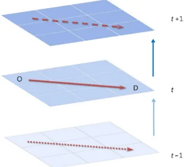
Traditional gravity or spatial interaction models focus on the impacts of origin- and destination-specific characteristics and the distance-decay effect on observed flows (Sen and Smith 1995; Mátyás 1997). Given this starting point, this study considers temporal dependence between adjacent time periods. For simplicity, we assume that migration flows in a given time period are dependent only on the immediate past period values, regardless of subsequent periods, as shown in Figure 1.

Introducing a first-order time lag of the dependent variable into the traditional gravity model allows us to determine a dynamic panel data model for migration flows as shown in Equation (1) (Parent and LeSage 2010, 2012):

= + × + + + + ,

= + × , (1)

where =( , … , ) consists of time periods of migration flows and

=( , … , ) is an ´1( = ) column vector of regional gross flows

(10)

= ( , … , ) are the explanatory variables at origins and destinations covering time periods where ( ) is formed by the Kronecker product ⊗ ( ⊗ ), is an × explanatory variable matrix for regions at the th time period, resulting in an × block matrix as the origin (destination) variable for all the flows; and

= ( , … , ), where represents the distance between all origins and destinations

at the th time period, in the form of time-invariant Euclidean distances or time-variant migration costs. The error term vector is decomposed into random individual effects and the disturbance vector × . The × 1 column vector captures individual

heterogeneities among migration flows with ~ (0, ), which change only with the individuals and are constant over time. The × is assumed to be uncorrelated with

and is identically distributed with zero mean and variance . , , , , and are the parameters to be estimated: is the intercept, and reflect the impacts associated with the origin- and destination-specific characteristics, denotes the impact of distance between different regions, and represents the magnitude of temporal dependence.

Figure 1: The temporal dependence structure of migration flows

Note: The OD migration flow in thetth time period in a red solid line is influenced by the previous flow in time periodt-1 in a red dotted line, and will exert a potential impact on the future flow in time periodt+1 in a red dashed line.

(11)

here accounts for more complicated temporal dependence and individual effects than the conventional gravity model can capture.

3.2 Spatial dynamic panel data model

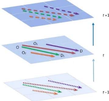
As explained in Section 1, migration is a path-dependent process. Any migration flow is influenced not only by origin- and destination-specific characteristics, but also by the same flow during the previous period (temporal dependence), the neighbouring flows in the current period (spatial dependence), and the neighbouring flows in the previous period (space-time diffusion dependence) (Parent and LeSage 2010, 2012; Mitze 2016). In short, unlike unidirectional temporal dependence (Figure 1), space-time dependence is multidimensional and multidirectional in nature (Figure 2).

Figure 2: The space-time dependence structure of migration flows

Note: The OD migration flow in thetth time period in a red solid line is influenced not only by the previous flow in time periodt-1 in a red dotted line (capturing temporal dependence) and the current neighbouring flows (O1D, OD1 and O2D1) in purple, green, and

orange solid lines (representing origin-, destination-, and origin-to-destination-based spatial dependence, respectively), but also by the previous neighbouring flows in purple, green, and orange dotted lines (representing origin-, destination-, and origin-to-destination-based space-time dependence, respectively). Furthermore, the current flows will exert potential impacts on the flows in future time periodt+1 in dashed lines of different colours.

(12)

(2008, 2009). Assuming is the × spatial weight matrix with zeros on the diagonal, these three types of spatial dependence are defined by the corresponding network weight matrices , , and : = ⊗ , = ⊗ , and =

⊗ (Chun 2008; LeSage and Pace 2008, 2009; LeSage and Llano 2013; Griffith, Fischer, and LeSage 2017).

Based on the spatial dependence of migration flows, we then define another three types of space-time diffusion dependence. If a migration flow in a given time period is influenced by flows from neighbouring origins to the same destination in the time period immediately preceding it, this can be understood as origin-based space-time dependence. Similarly, destination- and origin-to-destination-based space-time dependence of migration flows can be accordingly defined.

We now extend the general dynamic panel data model with the above spatial dependence and space-time diffusion dependence to derive a spatial dynamic panel data model of migration flows (Equation 2):

= ( ⊗ ) + ( ⊗ ) + ( ⊗ ) + + ( ⊗ )

+ ( ⊗ ) + ( ⊗ ) + × + +

+ + ,

= + × , (2)

where is the -dimensional identity matrix; the Kronecker products ⊗ , ⊗ , and ⊗ represent the space-time weight matrices for all migration flows over time periods; ( ⊗ ) ,( ⊗ ) , and ( ⊗ ) , accordingly, represent origin-, destination-, and origin-to-destination-based spatial lags of migration flows in corresponding time periods; ( ⊗ ) , ( ⊗ ) , and ( ⊗ )

represent origin-, destination-, and origin-to-destination-based space-time lags of migration flows. Like the scalar parameter of temporal dependence, ( , , ) and ( , , ) measure the strength of the spatial dependence and space-time diffusion dependence, respectively.

(13)

, , , , , , , , , , , , ∝ ( |Υ, , , , , )

(Υ) ( ) ( ) ( ) ( ),(3)

where Υ= ( , , , ), = ( , , ), and = ( , , ); ( | ⋅) represents the likelihood function; and (⋅) represents the prior distribution of each parameter.

The samples drawn from the set of conditional posterior distributions by the MCMC sampling method are used to estimate the associated parameters and their significance. The specific MCMC sampling and updating scheme for the spatial dynamic panel model are presented in the Appendix.

3.3 Interpreting the space-time effects of migration processes

For a spatial dynamic panel data model, a change in regional characteristics not only has a direct influence on the outflows and inflows from and to this region, but also has an indirect effect on the flows to and from other regions in the migration network over space and time. Therefore, there is a need to quantify various responses in the network from a local perspective (Golgher and Voss 2016). Following LeSage and Thomas-Agnan (2015), we extend the scalar summary measures of origin, destination, intraregional, and spillover effects to a space-time context and decompose them into contemporaneous, short-, and long-term components to reveal the changing impacts over time.

A change in a typical region at any time will potentially bring about transitory impacts on the flows during the period + to different degrees. Specifically, total effects (TE) are the impacts on all flows in the manner of × partial derivatives shown in Equation (4) (Debarsy, Ertur, and LeSage 2012; LeSage and Thomas-Agnan 2015):

=

⎝ ⎜ ⎛

⋮ ⎠ ⎟ ⎞

=

⎝ ⎜ ⎜

⎛ ( )/ ( )

( )/ ( ) ⋮

( )/ ( )⎠ ⎟ ⎟ ⎞

=

⎝ ⎜

⎛ +

+

⋮

+ ⎠

⎟ ⎞

,

= (−1) ( ) , (4)

= − − − ,

=−( + + + ),

(14)

interactions. is an × matrix of zeros with the th column equal to , and is an × matrix of zeros with the th row equal to ( = 1, … , ). Thus, the rows of the matrix ( ( )/ ( )) record the impacts on inflows to region , and its columns record the impacts on outflows from region . That is, each element corresponds to the change of different flows concerning region in detail.

Accordingly, we can calculate the cumulative total effects (CTE) over all time periods using Equation (5):

=

⋮ =

⎝ ⎜

⎛ ( ~ )/ ( )

( ~ )/ ( ) ⋮

( ~ )/ ( )_⎠ ⎟ ⎞

=∑

⋮

. (5)

A special case is the contemporaneous effect (T= 0), which is caused only by spatial interactions without temporal dependence. As time passes, tends to be infinite and the cumulative long-term effects tend to be stable. In this circumstance, approaches 0 and∑ = ( + ) .

Furthermore, the scalar summary measure of total effects ( ), expressed by the average of the total impacts on all flows in the network, can be calculated as: =

1/ ⋅ ⋅ ⋅ .

Analogously, a scalar summary measure of origin effects ( ) can be based on

= 1/ ⋅ ⋅ ⋅ , where is then2_´_{n matrix defined in Equation (6):}

=

⋮ =∑ ⋮

, (6)

where is then´n matrix that adjusts the element (i,i) in to zero for the purpose of separating the intraregional effect. The adjusted matrix allows for only (n - 1) changes in outflows from regioni as an origin in the OD dyad.

A scalar summary measure of destination effects ( ) can be based on = 1/ ⋅ ⋅ ⋅ , where is then2_´_{n matrix defined in Equation (7):}

=

(15)

where is then ´n matrix that adjusts the element (i,i) in to zero without the intraregional effect. This matrix allows for only (n- 1) changes in inflows to regioni as a destination.

A scalar summary measure for the intraregional effects ( ) can be based on

= 1/ ⋅ ⋅ ⋅ , where is then2_´_{n matrix defined in Equation (8):}

=

⋮ =∑

( )

⋮

( )

, (8)

where is ann´nmatrix of zeros with a ‘1’ in element (i,i).

The scalar summary measure for the cumulated spillover effects ( ) can be calculated as ≡ − − − . More generally, spatial effects can be expressed using = 1/ ⋅ ⋅ ⋅ , where is an n2 _´ _{n matrix, by setting all the}

elements of the th row and the th column of each in to 0.

In the nonspatial dynamic panel model,( , , ) and( , , ) are set to 0 and the spillover effects dissolve into nothingness.

4. Results

To illustrate our model of space-time dynamics within a migration network, we applied a panel data set of 5,580 gross migration flows between 31 mainland provinces in China (excluding intra-provincial migration flows) over six time periods between 1985 and 2015 (each time period equals five years). Migration flow data were collected from three population censuses (NBSC 1993, 2002, 2012) and three 1% population sample surveys (NBSC 1997, 2007, 2016). For consistency, migration flows to and from Chongqing during 1985–1990 and 1990–1995 were imputed based on its corresponding proportion of the population of Sichuan, since Chongqing was upgraded to a centrally administered municipality from a city of Sichuan province in 1997. Similarly, the missing migration flows to and from the Tibet Autonomous Region during 1985–1990 were also imputed from those of the adjacent time periods, since those data were not available in the 1990 census.

(16)

2016, 2017). Population size, as a typical gravity variable, has been demonstrated as effective in driving continued migration flows in China since the late 1970s (Fan 2005). The signs of population size at the origin and destination are expected to be positive, indicating push-pull forces between origins and destinations. GDP at the origin and destination is used to test the impact of regional economic disparity on stimulating migration flows. The expected signs of GDP at the origin and destination are negative and positive, respectively, suggesting people will move from a relatively poor region to a developed one. Age structure, measured by the proportion of working-age population (ages 15-64), reflects the predominance of labour migration. According to the 2015 1% population survey, labour population accounted for more than 85% of migrants during the 2010-2015 period (NBSC 2016). The signs of age structure at the origin and destination are expected to be positive and negative, respectively, indicating migrants are moving from labour-supplying regions to labour-demanding ones. Real wages as a measure of regional economic opportunity are the main motivation for mobility. We expect that the signs of real wages at the origin and destination are opposite, meaning that people will move to a region with higher income from a region with lower income. Compared with the constant railway distance, travel time can reflect improvement in transportation infrastructure. A negative decay effect of time distance is expected.

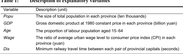
We use a log transformation of both dependent variable and explanatory variables to interpret the space-time effects as elasticities. To avoid the endogeneity problem, we lagged the dependent variable and explanatory variables by five years (LeSage and Pace 2008; Patuelli and Arbia 2016). Thus, the lagged migration flows at the initial period (1985-1990) were taken from the 1987 1% population sample survey (NBSC 1988), while data on regional population size, GDP, the proportion of labour force population, and real wages were collected from the China Statistical Yearbook on the first year of their corresponding periods (NBSC 1986, 1991, 1996, 2001, 2006, 2011). The minimum travel time by railway was collected from the China Railway Timetable at the same base year as the other exogenous explanatory variables (TBMR 1985, 1990, 1995, 2000, 2005, 2010). To check for the problem of potential multicollinearity, we calculate the variance inflation factor (VIF) for all variables (under 2.50), indicating no serious multicollinearity in our model. Table 1 describes these explanatory variables in detail.

We construct the spatial weight matrix based on the first-order contiguity, reflecting whether a common boundary exists between two provinces, denoted by 0 or 1. Since Hainan province is an island that once belonged to Guangdong province, we designate Guangdong as its neighbour. The spatial weight matrix W is then row-normalized to produce three different network weight matrices , , and . In practice, we remove the diagonal elements from , , and to derive the ×

(17)

estimates and inferences, consistent with LeSage and Pace (2014), and hence we focus on the results from the first-order contiguity matrix.

Table 1: Description of explanatory variables

Variable Description (unit)

Popu The size of total population in each province (ten thousands)

GDP Gross domestic product at 1980 constant price in each province (billion yuan)

Age The proportion of labour population aged 15-64

Wage The ratio of average urban wage level to consumer price index (CPI) in each

province (yuan)

Dis Minimum railway travel time between each pair of provincial capitals (seconds)

Source: NBSC (1986, 1991, 1996, 2001, 2006, 2011); TBMR (1985, 1990, 1995, 2000, 2005, 2010).

4.1 Model parameter estimates

(18)

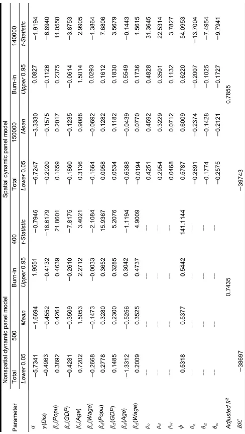
Table 2: Parameter estimates for nonspatial and spatial dynamic panel models Param eter Non spatial d ynam

ic panel m

(19)

In general, the spatial dynamic panel data model is superior to the nonspatial one in characterizing the Chinese interprovincial migration process during 1985-2015, as seen by its smaller BIC (Bayesian Information Criterion) value. Furthermore, Chinese interprovincial migration is a path-dependent process, as demonstrated by the fact that temporal, spatial, and space-time diffusion dependencies are significantly different from zero. The significant and positive temporal dependence ( ) indicates that past migrants tend to produce future sustained outflows and inflows. In China, migration flows are usually dependent on social linkages, such as relying on family members, friends, or fellow-townspeople for job opportunities (Liu 2014). Even if an entire family moves, their migration process is often unsynchronized. It is the positive network externalities that make subsequent migrants follow the path blazed by the pioneers, giving rise to strong temporal dependence during migration processes (Epstein 2008). Surprisingly, temporal dependence has been strengthened by including space-time interactions in the spatial dynamic panel data model, rather than the contrary, reflecting network externalities’ possible interaction with herd effects.

The significant and positive spatial dependence parameters (ro, rd, and rw) can

corroborate the existence of herd effects during the development of migration flows (Epstein 2008). The origin-, destination-, and origin-to-destination-based spatial dependencies represent three different but complementary migration paths. Specifically, the origin-based path implies that migration flows from the origin to the destination may promote outflows from surrounding origins to the same destination. Similarly, migration flows from the origin (or neighbouring origins) to neighbouring destinations are also enhanced, as implied by the destination-based (or origin-to-destination-based) path. Comparatively, the origin-based path dominates the other two; the largest spatial dependence (ro = 0.4592) is further supported by the fact that origins with strong

outflows are mainly located in China’s central and western regions. Like the time decay effect, the strength of origin-, destination-, and origin-to-destination-based spatial dependences of less than 1 further corroborates the distance-decay effects over space.

(20)

phenomenon fully reflects the self-adjustment and adaptability of a complex migration system, which involves much more complicated processes than the nonspatial model suggests.

Distance, as measured by minimum railway travel time, has significant and negative effects, as expected. Notably, the distance-decay effect in the spatial dynamic panel data model is significantly reduced compared with that in the nonspatial model, since spatial dependence can play a role similar to that of distance (LeSage and Thomas-Agnan 2015). Although the rapid progress of transportation technology has greatly facilitated migration activity, longer distances and higher time costs still restrict people’s aspirations to migrate, as does the relative scarcity of information about distant regions (Huff and Jenks 2015).

The coefficient estimates of explanatory variables in the spatial dynamic panel data model should not be directly interpreted as partial derivative impacts of regional factors on migration flows. To better understand the space-time dynamics in determining interprovincial migration processes in China, we perform a comprehensive quantitative analysis by calculating various space-time effects of explanatory variables and drawing valid inferences about their statistical significance.

4.2 Analysis of space-time effects

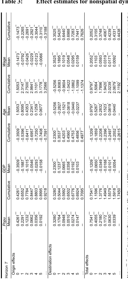
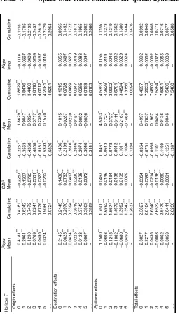
Tables 3 and 4 show various effect estimates of regional population size, GDP, age structure, and real wages in the nonspatial and spatial dynamic panel data models, respectively. The rows labelled ‘0’ represent the immediate responses of migration flows to changes in regional characteristics in terms of contemporaneous effects. The following rows labelled between ‘1’ and ‘5’ capture the disaggregated period-by-period impacts on the follow-on migration flows at different time periods. The last rows labelled ‘…’ reflect the cumulative long-term effects. The columns labelled ‘Mean’ record the means of the transitory period-by-period effects and the columns labelled ‘Cumulative’ the accumulated effects from the initial period to the current period.

(21)

migration flows but also stimulate a more lasting and sustained influence on the whole system.

Table 3: Effect estimates for nonspatial dynamic panel model

zon T Popu GDP A ge Wage Mean Cu m u lative Mean Cu m u lative Mean Cu m u lative Mean Cu m u lative Origin e ffects 0 0.426 1 *** 0.426 1 *** -0.350 9 *** -0.350 9 *** 1.505 3 *** 1.505 3 *** -0.147 3 ** -0.147 3 ** 1 0.229 1 *** 0.655 2 *** -0.188 7 *** -0.539 6 *** 0.809 5 *** 2.314 7 *** -0.079 2 ** -0.226 5 ** 2 0.123 2 *** 0.778 4 *** -0.101 5 *** -0.641 1 *** 0.435 3 *** 2.750 0 *** -0.042 6 ** -0.269 1 ** 3 0.066 2 *** 0.844 7 *** -0.054 6 *** -0.695 7 *** 0.234 1 *** 2.984 1 *** -0.022 9 ** -0.292 1 ** 4 0.035 6 *** 0.880 3 *** -0.029 3 *** -0.725 0 *** 0.125 9 *** 3.1 101 *** -0.012 3 ** -0.304 4 ** 5 0.019 2 *** 0.899 5 *** -0.015 8 *** -0.740 8 *** 0.067 7 *** 3.177 8 *** -0.006 6 ** -0.31 10 ** … --0.921 8 *** -0.759 1 *** --3.256 6 *** -0.318 8 ** Desti nation ef fects 0 0.328 0 *** 0.328 0 *** 0.230 0 *** 0.230 0 *** -0.525 6 -0.525 6 0.352 5 *** 0.352 5 *** 1 0.176 4 *** 0.504 4 *** 0.123 7 *** 0.353 7 *** -0.282 7 -0.808 3 0.189 5 *** 0.542 0 *** 2 0.094 8 *** 0.599 2 *** 0.066 5 *** 0.420 3 *** -0.152 1 -0.960 4 0.101 9 *** 0.644 0 *** 3 0.051 0 *** 0.650 2 *** 0.035 8 *** 0.456 0 *** -0.081 8 -1.042 2 0.054 8 *** 0.698 8 *** 4 0.027 4 *** 0.677 6 *** 0.019 2 *** 0.475 3 *** -0.044 0 -1.086 2 0.029 5 *** 0.728 3 *** 5 0.014 7 *** 0.692 4 *** 0.010 3 *** 0.485 6 *** -0.023 7 -1.109 9 0.015 9 *** 0.744 1 *** … --0.709 5 *** --0.497 7 *** -1.137 4 --0.762 6 *** Total effects 0 0.754 1 *** 0.754 1 *** -0.120 9 *** -0.120 9 *** 0.979 7 * 0.979 7 * 0.205 2 *** 0.205 2 *** 1 0.405 5 *** 1.159 6 *** -0.065 0 *** -0.185 9 *** 0.526 7 * 1.506 4 * 0.1 103 *** 0.315 5 *** 2 0.218 0 *** 1.377 6 *** -0.034 9 *** -0.220 8 *** 0.283 2 * 1.789 6 * 0.059 3 *** 0.374 8 *** 3 0.1 172 *** 1.494 9 *** -0.018 8 *** -0.239 6 *** 0.152 3 * 1.942 0 * 0.031 9 *** 0.406 7 *** 4 0.063 0 *** 1.557 9 *** -0.010 1 *** -0.249 7 *** 0.081 9 * 2.023 9 * 0.017 1 *** 0.423 9 *** 5 0.033 9 *** 1.591 8 *** -0.005 4 *** -0.255 2 *** 0.044 0 * 2.067 9 * 0.009 2 *** 0.433 1 *** … --1.745 0 *** -0.261 5 *** --2.1 192 * --0.443 8 *** ***, **, and *deno te si gnificance at the 1%, 5%, and 10% levels, resp ectively. Interv al va lues of variou s effect es tim ates as w ell as m ean and cum ul ati ve

ues can be obta

ined from

the a

uthors upon

req

(22)

Table 4: Space-time effect estimates for spatial dynamic panel model Hori zon T Popu GDP A ge Wage Mean Cu m u lative Mean Cu m u lative Mean Cu m u lative Mean Cu m u lative Origin e ffects 0 0.418 1 *** 0.418 1 *** -0.225 7 *** -0.225 7 *** 1.862 9 *** 1.862 9 *** -0.1 118 -0.1 118 1 0.206 1 *** 0.624 2 *** -0.130 7 *** -0.356 3 *** 0.984 7 *** 2.847 6 *** -0.066 7 -0.178 5 2 0.123 0 *** 0.747 2 *** -0.079 5 *** -0.435 8 *** 0.592 4 *** 3.440 0 *** -0.040 9 -0.219 3 3 0.076 9 *** 0.824 1 *** -0.050 1 *** -0.485 8 *** 0.371 7 *** 3.81 16 *** -0.025 9 -0.245 2 4 0.049 5 *** 0.873 6 *** -0.032 3 *** -0.518 1 *** 0.239 5 *** 4.051 2 *** -0.016 7 -0.261 9 5 0.032 4 *** 0.906 0 *** -0.021 2 *** -0.539 3 *** 0.157 0 *** 4.208 1 *** -0.01 10 -0.272 9 … --0.972 4 *** -0.582 6 *** --4.529 1 *** -0.295 4 Desti nation ef fects 0 0.214 5 *** 0.214 5 *** 0.143 6 *** 0.143 6 *** 0.101 5 0.101 5 0.095 5 0.095 5 1 0.082 5 *** 0.297 0 *** 0.076 3 *** 0.219 9 *** -0.028 7 0.072 8 0.049 7 0.145 2 2 0.042 4 *** 0.339 4 *** 0.041 7 *** 0.261 6 *** -0.023 0 0.049 9 0.027 0 0.172 2 3 0.022 5 *** 0.361 9 *** 0.023 0 *** 0.284 6 *** -0.015 1 0.034 7 0.014 9 0.187 1 4 0.012 3 *** 0.374 2 *** 0.012 8 *** 0.297 4 *** -0.009 2 0.025 5 0.008 3 0.195 5 5 0.006 7 *** 0.380 9 *** 0.007 2 *** 0.304 6 *** -0.005 6 0.019 9 0.004 7 0.200 2 … --0.388 9 *** --0.314 1 *** --0.010 3 --0.206 6 Spillove r ef fects 0 1.750 0 *** 1.750 0 *** 0.046 7 0.046 7 4.535 3 ** 4.535 3 ** 0.1 155 0.1 155 1 -0.060 8 1.689 2 *** 0.014 6 0.061 3 -0.172 4 4.362 9 * 0.01 18 0.127 3 2 -0.121 8 ** 1.567 4 *** 0.016 4 0.077 8 -0.372 7 * 3.990 2 * 0.004 6 0.131 9 3 -0.100 2 *** 1.467 2 *** 0.013 5 0.091 2 -0.31 11 ** 3.679 1 * 0.003 2 0.135 2 4 -0.068 0 *** 1.399 2 *** 0.010 5 0.101 7 -0.216 7 *** 3.462 4 * 0.002 9 0.138 0 5 -0.045 0 *** 1.354 2 *** 0.007 9 0.109 6 -0.146 8 *** 3.315 6 * 0.002 4 0.140 4 … --1.263 7 *** --0.128 8 --3.009 4 * --0.147 6 Total effects 0 2.382 7 *** 2.382 7 *** -0.035 4 -0.035 4 6.499 7 ** 6.499 7 ** 0.099 2 0.099 2 1 0.227 7 2.610 4 *** -0.039 7 -0.075 1 0.783 7 7.283 3 ** -0.005 2 0.094 0 2 0.043 6 2.654 0 *** -0.021 4 ** -0.096 5 0.196 7 7.480 0 ** -0.009 2 0.084 8 3 -0.000 8 2.653 2 *** -0.013 6 *** -0.1 101 0.045 4 7.525 4 ** -0.007 7 0.077 1 4 -0.006 2 2.647 0 *** -0.008 9 *** -0.1 190 0.013 6 7.539 1 ** -0.005 5 0.071 6 5 -0.005 9 *** 2.641 1 *** -0.006 1 *** -0.125 1 0.004 6 7.543 6 ** -0.003 9 0.067 7 … --2.625 0 *** -0.139 7 --7.548 8 ** --0.058 8 Notes: *** , **, and *denote si gnificance at the 1%, 5%, and 10% levels, resp ec tiv el y. Interv al va lues of variou s effect estim ates as w el l as m ean and cum ul ati ve val

ues can be obta

ined from

the a

uthors upon

req

(23)

4.2.1 Population size

Population size is often chosen as the basic explanatory variable to characterize regional mass in traditional gravity models (Zipf 1946; Stillwell 2008). Migration flows between origins and destinations are positively proportional to their population sizes if other variables are held constant. Tables 3 and 4 show that, as hypothesized, the origin and destination effects of population size are significantly positive, exerting strong push and pull forces on interprovincial migration in China from 1985 to 2015. In addition, the cumulative origin and destination effects of population size continue to increase over time, indicating that changes in regional population have profound impacts on migration flows. The origin effects of population size are larger than the corresponding destination effects, reflecting the fact that the pressure from large populations is much stronger than their agglomeration effects during the migration process. In a typical region, a 1% increase in population size produces 0.42% more outflow during the same period. As time passes, transitory responses remain significantly positive, eventually leading to 0.97% additional outflow over the long term. On the other hand, a 1% increase in population size in a typical region produces 0.21% more inflow during the same period and 0.39% additional inflow in the long run, less than half of its long-term origin effect.

More importantly, changes in regional population size also impact the inflows and outflows to and from other regions through the migration network over time. It is these complex spillover effects that demonstrate the close link between migration flows. The spatial dynamic panel data model allows us to measure these invisible effects; the magnitude of such effects is beyond our expectations. Specifically, the cumulative spillover effects at different time periods are greater than 1.0, indicating a more rapid increase of migration flows arising from the same population growth across the network. On average, if a given population size in a typical region increases by 1%, the migration flows between other provinces will increase by 1.75% over the same period, well beyond the increase of outflows and inflows from and to the given region. This kind of spillover effect occurring at the same time (herd effect) may cause large flows even before networks are created, providing a complementary explanation for the formation of migration flows (Epstein 2008). As time passes, negative feedback effects in the following periods gradually weaken the cumulative network effects and eventually lead to a long-term effect of 1.2637, over two-thirds of its contemporaneous effect. These negative network externalities are also consistent with the reality that the number of immigrants may gradually reduce as the increase in new arrivals results in more competition for jobs. Declining network effects may help prevent the migration system from becoming out of control.

(24)

in Table 4 show that population size has the second largest impact on Chinese interprovincial migration flows. On average, a 1% increase in regional population in a typical region increases migration flows by 2.38% during the same period and by 2.63% over the long term. Although the spillover effects of population may decrease over time, they are still greater than its origin and destination effects. In other words, we cannot ignore the role of spillover effects in addition to traditional push and pull forces on the formation and development of migration flows.

4.2.2 GDP

Unbalanced regional economic development in China has led to continuing internal migration flows since the late 1970s (Cai and Wang 2003; Zhu 2003; Fan 2005). Tables 3 and 4 show that regional GDP plays a significant role in causing people to move between different areas, consistent with the neoclassical migration theory (Sjaastad 1962). The negative origin effects’ inhibiting role is strong during the initial period. On average, a 1% increase in regional GDP produces 0.23% less outflow in the same period (T= 0). As time passes the period-by-period effects decrease but remain significant. Over the long run the origin effect of GDP reaches -0.5826, an absolute value much larger than that of GDP during the contemporaneous period. In other words, regional economic development tends to reduce migration outflows over time.

As expected, the development of a regional economy attracts more immigrants, as evidenced by the significant and positive destination effects of GDP. On average, a 1% increase in GDP in a typical region attracts 0.14% more inflows during the same period and 0.08% more inflows during the following period (T = 1). Although the period-by-period effects appear to decay over time, the cumulative effect still reaches 0.3141 over the long term, twice that of the contemporaneous effect. If we do not consider the space-time interactions among migration flows (Table 3), most of the destination effects of GDP tend to be overestimated, thus ignoring the self-adjustment of migration processes.

(25)

Overall, the total effects of regional GDP can help explain the inverted U-shape relationship between development and migration. After sustained and rapid growth of interprovincial migration, China has experienced a declining trend since 2010 (NBSC 1993, 1997, 2002, 2007, 2012, 2016). Furthermore, the period-by-period effects of regional GDP for the contemporaneous time period out to one time horizon (T= 1) are not significantly different from zero, indicating that development may not necessarily decrease migration flows. In reality, regional economic development, at least in the initial time periods, may enhance migration because development enables and inspires people to move (Zelinsky 1971, De Haas 2007, 2010b). However, the transitory period-by-period effects of regional GDP are significant from the two time horizons (T= 2) on, reflecting that development does have a lagged decaying effect on migration.

4.2.3 Age structure

The labour force population is the most influential driver of migration flows. According to population censuses and national survey data (NBSC 1993, 1997, 2002, 2007, 2012, 2016), migrant workers dominate in the total migration population. From Table 4 we see that the origin effects of the proportion of working age population are the largest of all the explanatory variables, consistent with the nonspatial model estimates. The impact of a 1% increase in working age population at origin would result in a 1.86% increase in outflows during the same period and eventually a 4.53% outflow increase, more than four times the origin effects of population size. The enhancement of origin effects in the spatial model is the result of feedback effects arising from changes in network flows associated with regions neighbouring each OD dyad. The small magnitude of destination effects suggests that an increase in the proportion of local labour population does not significantly attract more foreigners to move in, indicating that its agglomeration effects are rather limited.

(26)

flows to other provinces throughout the migration network, making it a remarkable driving force.

Overall, interprovincial migration flows in China are extremely sensitive to the age structure of the population. Specifically, if the proportion of working age population in a typical region increases (or decreases) by 1%, there will be an increase (or decrease) of migration flows by 6.50% during the same period and by 7.55% over the long-term. That is, a slight change in the age structure of a regional population will have a great influence on current and future flows, especially in the contemporaneous period. This suggests that herd effects may dominate in migration processes, in line with the employment-oriented long-distance migration trends (Thomas, Gillespie, and Lomax 2019).

4.2.4 Real wages

A large number of migration studies indicate that people migrate to seek better job opportunities and to increase their quality of life (Chi and Voss 2005; Yue et al. 2010; Chen and Wang 2018). Without the consideration of space-time interactions, real wages do play a dominant role in the Chinese interprovincial migration process, as evidenced by various effect estimates shown in Table 3. However, this is not the case in the spatial model. We can see from Table 4 that the effect estimates of real wages are no longer significant, reflecting that real wages are not as important as expected in migration processes. These empirical results confirm that migrants are willing to give up higher wages initially, but prefer to move to more prosperous regions over time (Epstein 2008).

(27)

5. Conclusions

Migration is arguably playing an increasingly important role in regional growth and development than ever before. To understand the space-time dynamics of complex migration processes, this study constructs a spatial dynamic panel data model by incorporating temporal, spatial, and space-time diffusion dependencies into traditional gravity models. Moreover, we decompose origin, destination, and spillover effects into their contemporaneous, short-, and long-term components, thereby providing the tools to quantify the transitory and cumulative responses of migration flows to changes in regional characteristics. We then apply this model to interprovincial migration flows between 31 mainland provinces in China from 1985 to 2015, choosing population size, GDP, age structure, real wages at origin and destination, and railway travel time between provincial capitals as explanatory variables. To evaluate the importance of space-time interactions, we use a general (nonspatial) dynamic panel data model as a benchmark specification. Finally, we employ Bayesian MCMC procedures to estimate various effects and draw valid inferences regarding the mechanisms of Chinese interprovincial migration processes.

Our empirical results show that the spatial dynamic panel data model is more suitable for characterizing the path-dependent migration process. Past migrants tend to produce sustained outflows and inflows, as evidenced by more strong temporal dependence. Moreover, the origin-, destination-, and origin-to-destination-based paths complement one another during the generation and development of migration flows, as confirmed by the significant and positive spatial dependence. Comparatively, the origin-based path dominates the other two. However, the origin-, destination-, and origin-to-destination-based space-time paths provide different channels with which to adjust migration flows, as reflected by significant and negative space-time diffusion interactions. The origin-based space-time path is likely to be the most effective way to adjust the migration system toward an equilibrium state. Migration flows are perpetuated by the inertia of positive temporal and spatial dependence as well as by negative space-time diffusion dependence.

(28)

than the sum of origin and destination effects, indicating that herd and network externality effects dominate in the migration system. Third, the inverted U-shape relationship between development and migration can be partly explained by the total effects of regional GDP. Finally, the role of real wages in driving migration flows is rather weak, suggesting that migrants are willing to give up higher wages initially but prefer prosperous regions in the long run.

The gravity model remains popular within the field of migration studies (O’Kelly 2004). Adding space-time components to this model will not only help promote theoretical, methodological, and empirical aspects of migration modelling, but also advance its application in other spatial interaction modelling areas such as transportation and international and interregional trade. More importantly, temporal, spatial, and space-time dependencies represent inertia in a system: Monitoring and observing their presence will help us understand the vulnerability and resilience of a regional system (Griffith and Chun 2015). In a rapidly changing society it is of critical importance to be able to predict what will happen to a regional migration system under shock, and how to respond. The space-time framework can be applied to forecast future migration flows as well as to explain past and present processes (Baltagi, Fingleton, and Pirotte 2019).

The spatial dynamic panel approach proposed in this study is a powerful means to understand how migration flows respond to regional socioeconomic changes and how space and time influence migration processes. However, the various coefficient and effect estimates are computationally expensive because more parameters are involved in the spatial model: Practical parallel strategies need to be tested. In addition, we only considered global spillover effects with a dependent variable lagged in both space and time: Possible local spillover effects can be investigated in a spatial dynamic Durbin panel model. Furthermore, we ignored model uncertainty in the selection of explanatory variables: The Bayesian model averaging method can be further explored with more regional social, economic, and environmental factors. Overall, to track the complex evolution of a regional migration system in future research, other types of spatial-temporal models for dyadic flow data should be specified, interpreted, and calibrated.

6. Acknowledgements

(29)

References

Anselin, L., Le Gallo, J., and Jayet, H. (2008). Spatial panel econometrics. In: Mátyás, L. and Sevestre, P. (eds.). The econometrics of panel data: Fundamentals and recent developments in theory and practice. Berlin: Springer: 625‒660.

doi:10.1007/978-3-540-75892-1_19.

Baláž, V. and Williams, A.M. (2007). Path-dependency and path-creation perspectives on migration trajectories: The economic experiences of Vietnamese migrants in Slovakia. International Migration 45(2): 37-66.doi:10.1111/j.1468-2435.2007. 00403.x.

Baltagi, B.H., Fingleton, B., and Pirotte, A. (2019). A time-space dynamic panel data model with spatial moving average errors. Regional Science and Urban Economics 76: 13-31.doi:10.1016/j.regsciurbeco.2018.04.013.

Bauer, T., Epstein, G.S., and Gang, I.N. (2007). The influence of stocks and flows on migrants’ location choices. Research in Labor Economics 26: 199-229.

doi:10.1016/S0147-9121(06)26006-0.

Bavaud, F., Kordi, M., and Kaiser, C. (2018). Flow autocorrelation: A dyadic approach. Annals of Regional Science 61(1): 95-111.doi:10.1007/s00168-018-0860-y. Beenstock, M. and Felsenstein, D. (2019).The econometric analysis of non-stationary

spatial panel data. Switzerland: Springer.doi:10.1007/978-3-030-03614-0. Bellos, S. and Subasat, T. (2012). Governance and foreign direct investment: A panel

gravity model approach. Bulletin of Economic Research 64(4): 565–574.

doi:10.1111/j.1467-8586.2010.00370.x.

Bernard, A. (2017). Cohort measures of internal migration: Understanding long-term trends.Demography 54(6): 2201-2221.doi:10.1007/s13524-017-0626-7. Bhargava, A. and Sargan, J.D. (1983). Estimating dynamic random effects models from

panel data covering short time periods. Econometrica 51(6): 1635-1659.

doi:10.2307/1912110.

Biagi, B., Faggian, A., Rajbhandari, I., and Venhorst, V.A. (2018). New frontiers in interregional migration research. Cham: Springer International Publishing.

doi:10.1007/978-3-319-75886-2.

(30)

Black, W. (1992). Network autocorrelation in transportation network and flow systems. Geographical Analysis 24(3): 207-222. doi:10.1111/j.1538-4632.1992.tb00 262.x.

Cai, F. and Wang, D. (2003). Migration as marketization: What can we learn from China’s 2000 census data?China Review 3(2): 73–93.

Chen, J. and Wang, W. (2018). Economic incentives and settlement intentions of rural migrants: Evidence from China. Journal of Urban Affairs 41(3): 372–389.

doi:10.1080/07352166.2018.1439339.

Chi, G. and Voss, P.R. (2005). Migration decision-making: A hierarchical regression approach. Journal of Regional Analysis and Policy 35(2): 11–22.

Chib, S. and Carlin, B.P. (1999). On MCMC sampling in hierarchical longitudinal models.Statistics and Computing 9(1): 17-26.doi:10.1023/A:1008853808677. Chort, I. and de la Ruppelle, M. (2016). Determinants of Mexico–U.S. outward and

return migration flows: A state-level panel data analysis. Demography 53(5): 1453-1476.doi:10.1007/s13524-016-0503-9.

Chun, Y. (2008). Modeling network autocorrelation within migration flows by eigenvector spatial filtering. Journal of Geographical Systems 10(4): 317-344.

doi:10.1007/s10109-008-0068-2.

Chun, Y. and Griffith, D. (2011). Modeling network autocorrelation in space–time migration flow data: An eigenvector spatial filtering approach. Annals of the Association of American Geographers 101(3): 523-536. doi:10.1080/00045 608.2011.561070.

Church, J. and King, I. (1993). Bilingualism and network externalities. The Canadian Journal of Economics 26(2): 337-345.doi:10.2307/135911.

Crown, D., Jaquet, T., and Faggian, A. (2018). Interregional migration and implications for regional resilience. In: Biagi, B., Faggian, A., Rajbhandari, I., and Venhorst, V.A. (eds.). New frontiers in interregional migration. Cham: Springer International Publishing: 231-252.doi:10.1007/978-3-319-75886-2_11.

Cushing, B. and Poot, J. (2003). Crossing boundaries and borders: Regional science advances in migration modelling. Papers in Regional Science 83(1): 317-338.

doi:10.1007/s10110-003-0188-5.

(31)

De Haas, H. (2007). Turning the tide? Why development will not stop migration. Development and Change 38(5): 819-841. doi:10.1111/j.1467-7660.2007.004 35.x.

De Haas, H. (2010a). The internal dynamics of migration processes: A theoretical inquiry. Journal of Ethnic and Migration Studies 36(10): 1587-1617.

doi:10.1080/1369183X.2010.489361.

De Haas, H. (2010b). Migration and development: A theoretical perspective. International Migration Review 44(1): 227-264.doi:10.1111/j.1747-7379.2009. 00804.x.

Debarsy, N., Ertur, C., and LeSage, J. P. (2012). Interpreting dynamic space–time panel data models.Statistical Methodology 9(1): 158-171.doi:10.1016/j.stamet.2011. 02.002.

Elhorst, J.P. (2010). Spatial panel data models. In: Fischer, M.M. and Getis, A. (eds.). Handbook of applied spatial analysis: Software tools, methods and applications. Berlin: Springer: 377-407.doi:10.1007/978-3-642-03647-7_19.

Elhorst, J.P. (2012). Dynamic spatial panels: Models, methods and inferences.Journal of Geographical Systems 14(1): 5-28.doi:10.1007/s10109-011-0158-4.

Elhorst, J.P. (2014).Spatial econometrics: From cross-sectional data to spatial panels. London: Springer.doi:10.1007/978-3-642-40340-8.

Epstein, G.S. (2008). Herd and network effects in migration decision-making.Journal of Ethnic and Migration Studies 34(4): 567-583. doi:10.1080/13691830801 961597.

Etzo, I. (2011). The determinants of the recent interregional migration flows in Italy: A panel data analysis. Journal of Regional Science 51(5): 948–966.

doi:10.1111/j.1467-9787.2011.00730.x.

Fan, C.C. (2005). Modeling interprovincial migration in China, 1985–2000. Eurasian Geography and Economics 46(3): 165-184.doi:10.2747/1538-7216.46.3.165. Fotheringham, A.S. (1991). Migration and spatial structure: The development of the

competing destinations model. In: Stillwell, J. and Congdon, P. (eds.).Migration models: Macro and micro approaches. London: Belhaven Press: 57-72.

(32)

Greenwood, M.J. (1969). An analysis of the determinants of geographic labor mobility in the United States. Review of Economics and Statistics 51(2): 189-194.

doi:10.2307/1926728.

Greenwood, M.J. (1970). Lagged response in the decision to migrate. Journal of Regional Science 10(3): 375-384.doi:10.1111/j.1467-9787.1970.tb00059.x. Griffith, D.A. (2009). Spatial autocorrelation in spatial interaction:

Complexity-to-simplicity in journey-to-work flows. In: Reggiani, A. and Nijkanmp, P. (eds.). Complexity and spatial networks. Berlin: Springer: 221-237. doi:10.1007/978-3-642-01554-0_16.

Griffith, D.A. and Chun, Y. (2015). Spatial autocorrelation in spatial interactions models: Geographic scale and resolution implication for network resilience and vulnerability. Networks and Spatial Economics 15(2): 337-365. doi:10.1007/ s11067-014-9256-4.

Griffith, D.A. and Fischer, M.M. (2013). Constrained variants of the gravity model and spatial dependence: Model specification and estimation issues. Journal of Geographical Systems 15(3): 291-317.doi:10.1007/s10109-013-0182-7. Griffith, D.A., Fischer, M.M., and LeSage, J.P. (2017). The spatial autocorrelation

problem in spatial interaction modeling: A comparison of two common solutions. Letters in Spatial and Resource Sciences 10(1): 75-86. doi:10.1007/ s12076-016-0172-8.

Griffith, D.A. and Jones, K. (1980). Explorations into the relationships between spatial structure and spatial interaction. Environment and Planning A 12(2): 187-201.

doi:10.1068/a120187.

Huff, D.L. and Jenks, G.F. (2015). A graphic interpretation of the friction of distance in gravity models. Annals of the Association of American Geographers 58(4): 814-824.doi:10.1111/j.1467-8306.1968.tb01670.x.

Kau, J.B. and Sirmans, C.F. (1979). A recursive model of the spatial allocation of migrants. Journal of Regional Science 19(1): 47-56. doi:10.1111/j.1467-9787. 1979.tb00570.x.

Laber, G. (1972). Lagged response in the decision to migrate: A comment. Journal of Regional Science 12(2): 307-310.doi:10.1111/j.1467-9787.1972.tb00352.x. Lamonica, G.R. and Zagaglia, B. (2013). The determinants of internal mobility in Italy,

(33)

Lee, E.S. (1966). A theory of migration. Demography 3(1): 47-57. doi:10.2307/20 60063.

LeSage, J.P. (2010). Econometrics Toolbox. San Marcos: Texas State McCoy College of Business.http://spatial-econometrics.com.

LeSage, J.P. (2014). Spatial econometric panel data model specification: A Bayesian approach.Spatial Statistics 9: 122-145.doi:10.1016/j.spasta.2014.02.002. LeSage, J.P. and Fischer, M.M. (2016). Spatial regression-based model specifications

for exogenous and endogenous spatial interaction. In: Patuelli, R. and Arbia, G. (eds.).Spatial econometric interaction modelling. Cham: Springer International Publishing: 15-36.doi:10.1007/978-3-319-30196-9_2

LeSage, J.P. and Llano, C. (2013). A spatial interaction model with spatial structure origin and destination effects. Journal of Regional Science 15(3): 265-289.

doi:10.1007/s10109-013-0181-8.

LeSage, J.P. and Pace, R.K. (2008). Spatial econometric modeling of origin-destination flows. Journal of Regional Science 48(5): 941-967. doi:10.1111/j.1467-9787. 2008.00573.x.

LeSage, J.P. and Pace, R.K. (2009).Introduction to spatial econometrics. Boca Raton: CRC press.doi:10.1201/9781420064254.

LeSage, J.P. and Pace, R.K. (2014). The biggest myth in spatial econometrics. Econometrics 2(4): 217-249.doi:10.3390/econometrics2040217.

LeSage, J.P. and Thomas-Agnan, C. (2015). Interpreting spatial econometric origin-destination flow models. Journal of Regional Science 55(2): 188-208.

doi:10.1111/jors.12114.

Li, S. (2004). Population migration and urbanization in China: A comparative analysis of the 1990 population census and the 1995 national one percent sample population survey.International Migration Review38(2): 655-685.doi:10.1111/ j.1747-7379.2004.tb00212.x.

Liang, Z. and Song, Q. (2016). Migration in China. In: White, M.J. (ed.).International handbook of migration and population distribution. Dordrecht: Springer Science + Business Media: 285-309.doi:10.1007/978-94-017-7282-2_14.

(34)

Liu, Y. and Shen, J. (2014). Jobs or amenities? Location choices of interprovincial skilled migrants in China, 2000-2005. Population, Space and Place 20(7): 592-605.doi:10.1002/psp.1803.

Mátyás, L. (1997). Proper econometric specification of the gravity model.The World Economy 20(3): 363-368.doi:10.1111/1467-9701.00074.

Mátyás, L. (2017). The econometrics of multi-dimensional panels: Theory and applications. Cham: Springer International Publishing. doi:10.1007/978-3-319-60783-2.

Mavroudi, E. and Nagel, C. (2016).Global migration: Patterns, processes, and politics. London: Routledge.doi:10.4324/9781315623399.

Mitze, T. (2012). Empirical modelling in regional science: Towards a global time-space-structural analysis. Berlin: Springer.doi:10.1007/978-3-642-22901-5. Mitze, T. (2016). On the mutual dynamics of interregional gross migration flows in

space and time. In: Patuelli, R. and Arbia, G. (eds.). Spatial econometric interaction modelling. Berlin: Springer: 415-440. doi:10.1007/978-3-319-30196-9_16.

National Bureau of Statistics of China (NBSC). (1986). China statistics yearbook. Beijing: China Statistics Press.

National Bureau of Statistics of China (NBSC). (1988).Tabulations on the 1987 1% population sampling survey of the People's Republic of China. Beijing: China Statistics Press.

National Bureau of Statistics of China (NBSC). (1993). Tabulation on the 1990 population census of the People’s Republic of China. Beijing: China Statistics Press.

National Bureau of Statistics of China (NBSC). (1997). Tabulation on the 1995 1% population sampling survey of the People’s Republic of China. Beijing: China Statistics Press.

(35)

National Bureau of Statistics of China (NBSC). (2011). China Statistics Yearbook. Beijing: China Statistics Press.

Odland, J. and Shumway, J.M. (1993). Interdependencies in the timing of migration and mobility events. Papers in Regional Science 72(3): 221-237. doi:10.1007/BF0 1434274.

O’Kelly, M.E. (2004). Isard’s contributions to spatial interaction modelling.Journal of Geographical Systems 6(1): 43-54.doi:10.1007/s10109-004-0125-4.

Parent, O. and LeSage, J.P. (2010). A spatial dynamic panel model with random effects applied to commuting times. Transportation Research Part B 44(5): 633-645.

doi:10.1016/j.trb.2010.01.004.

Parent, O. and LeSage, J.P. (2012) Spatial dynamic panel data models with random effects. Regional Science and Urban Economics 42(4): 727-738. doi:10.1016/ j.regsciurbeco.2012.04.008.

Patuelli, R. and Arbia, G. (2016). Spatial econometric interaction modelling. Cham: Springer International Publishing.doi:10.1007/978-3-319-30196-9.

(36)

Plane, D.A. and Rogerson, P.A. (1986). Dynamic flow modeling with interregional dependency effects: An application to structural change in the U.S. migration system.Demography23(1): 91-104.doi:10.2307/2061411.

Rainer, H. and Siedler, T. (2009). The role of social networks in determining migration and labour market outcomes: Evidence from German Reunification.Economics of Transition 17(4): 739-767.doi:10.1111/j.1468-0351.2009.00365.x.

Rogers, A. (1990). Requiem for the net migrant. Geographical Analysis 22(4): 283-300.doi:10.1111/j.1538-4632.1990.tb00212.x.

Rogers, A., Willekens, F., Little, J., and Raymer, J. (2002). Describing migration spatial structure. Papers in Regional Science 81(1): 29-48. doi:10.1007/s101100 100090.

Sjaastad, L.A. (1962). The costs and returns of human migration.Journal of Political Economy 70(5): 80-93.doi:10.1086/258726.

Sen, A. and Smith, T.E. (1995).Gravity models of spatial interaction behavior. Berlin: Springer.doi:10.1007/978-3-642-79880-1.

Shen, J. (2015). Explaining interregional migration changes in china, 1985–2000, using a decomposition approach. Regional Studies 49(7): 1176-1192. doi:10.1080/ 00343404.2013.812783.

Shen, J. (2016). Error analysis of regional migration modeling.Annals of the American Association of Geographers 106(6): 1-15. doi:10.1080/24694452.2016.11977 67.

Shen, J. (2017). Modelling interregional migration in China in 2005–2010: The roles of regional attributes and spatial interaction effects in modelling error. Population, Space and Place 23(3): e2014.doi:10.1002/psp.2014.

Stillwell, J. (2008). Inter-regional migration modelling: A review. In: Poot, J., Waldorf, B., and van Wissen, L. (eds.). Migration and human capital. Cheltenham: Edward Elgar: 29-48.

Thomas, M., Gillespie, B., and Lomax, N. (2019). Variations in migration motives over distance. Demographic Research 40(38): 1097-1110. doi:10.4054/DemRes. 2019.40.38.