© European Geosciences Union 2006
Geophysicae
Long-term solar activity explored with wavelet methods
H. Lundstedt1, L. Liszka2, R. Lundin3, and R. Muscheler4
1Swedish Institute of Space Physics, Lund, Sweden 2Swedish Institute of Space Physics, Ume˚a, Sweden 3Swedish Institute of Space Physics, Kiruna, Sweden
4National Center for Atmospheric Research, Paleoclimatology, Boulder, USA
Received: 23 May 2005 – Revised: 7 November 2005 – Accepted: 14 December 2005 – Published: 23 March 2006
Abstract. Long-term solar activity has been studied with a set of wavelet methods. The following indicators of long-term solar activity were used; the group sunspot number, the sunspot number, and the14C production rate. Scalograms showed the very long-term scales of 2300 years (Hallstat cy-cle), 900–1000 years, 400–500 years, and 200 years (de Vries cycle). Scalograms of a newly-constructed14C production rate showed interesting solar modulation during the Maun-der minimum. Multi-Resolution Analysis (MRA) revealed the modulation in detail, as well as peaks of solar activity not seen in the sunspot number. In both the group sunspot number scalogram and the14C production rate scalogram, a process appeared, starting or ending in late 1700. This pro-cess has not been discussed before. Its solar origin is unclear. The group sunspot number ampligram and the sunspot number ampligram showed the Maunder and the Dalton min-ima, and the period of high solar activity, which already started about 1900 and then decreased again after mid 1990. The decrease starts earlier for weaker components. Also, weak semiperiodic activity was found.
Time Scale Spectra (TSS) showed both deterministic and stochastic processes behind the variability of the long-term solar activity. TSS of the14C production rate, group sunspot number and Mt. Wilson sunspot index and plage index were compared in an attempt to interpret the features and pro-cesses behind the long-term variability.
Keywords. Solar physics, astrophysics and astronomy (Magnetic fields) – History of Geophysics (Solar-planetary relationships) – Interplanetary physics (Cosmic rays)
1 Introduction
Solar activity drives space weather. Space weather can have a severe effect on technological systems (Lundstedt, 2005). Not only space-borne systems are affected, but terrestrial
Correspondence to: H. Lundstedt
systems, such as electrical power distribution grids and ter-restrial communications, as well. To mitigate the effects on long-term scales (decades and longer) it is therefore impor-tant to study the long-term solar activity. Because the cli-mate of the Earth owes its existence in large part to the Sun, it is also important to understand how it is changed due to the long-term solar activity (Muscheler et al., 2005a; Schlesinger and Andronova, 2003).
In Lundstedt (2001) predictions of solar activity based on Artificial Intelligence (Fu, 1994) methods is reviewed. A new approach of exploring, understanding and predicting so-lar activity was introduced in Lundstedt (2006). It is based on newly-developed wavelet methods and physics-based neural networks. New predictions of solar flares, based on neu-ral networks, have been developed by Jensen et al. (2004). The neural networks use both results from solar dynamo the-ory (Dikpati and Charbonneau, 1999) and helioseismology (Christensen-Dalsgaard and Thompson, 2003). The devel-oped wavelet methods were applied to short-term and mid-term solar activity indicators in Lundstedt et al. (2005). In this article we will apply wavelet methods to long-term solar activity, i.e. on a time scale of the main 11-year solar cycle and longer.
2 Indicators of long-term solar activity – Data
To study the solar activity changes over a period of 11 500 years (–9950 years BC–1950 AD) we have used the
14C production rate constructed from radiocarbon records
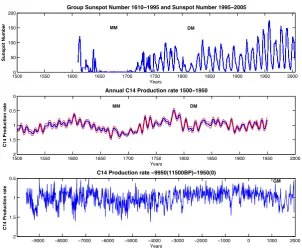
(Muscheler et al., 2004, 2005b). The data, with 10-year res-olution, is plotted in the lower panel of Fig. 1. A quick look tells us that the data looks different before about 5000 BC. Occasional occurrences of dropouts in14C production rate also take place before 0 AD. Times of the Grand maxi-mum (Middle Ages, ca. 1000–1200) and Maunder minimaxi-mum (ca. 1645–1715) are marked.
15000 1550 1600 1650 1700 1750 1800 1850 1900 1950 2000 50
100
Years
Sunspot Number
1500 1550 1600 1650 1700 1750 1800 1850 1900 1950 2000
0
0.5
1
1.5
2
Years
C14 Production rate
Annual C14 Production rate 1500−1950
MM DM
−9000 −8000 −7000 −6000 −5000 −4000 −3000 −2000 −1000 0 1000 2000 0.5
1
1.5
2
Years
C14 Production rate
C14 Production rate −9950(11500BP)−1950(0)
[image:2.595.147.450.71.323.2]GM
Fig. 1. Upper panel shows group sunspot numberRG 1610–1995 and sunspot numberRz 1995–2005. Middle panel shows the14C
production rate from 1500–1950. Lower panel shows the14C production rate from−9950 BC–1950. MM stands for Maunder Minimum, DM for Dalton Mimum and GM for Grand Maximum.
an annual resolution. The data is plotted in the middle panel of Fig. 1. The two red curves show the14C production rate
±1 sigma. The times of the Maunder minimum and the Dal-ton minimum (ca. 1795–1823) are marked.
In an attempt to further understand the variability of the
14C production we have compared the data with the group
sunspot number (Rg,1610–1995) and sunspot number (Rz,
1995–2005). The data is plotted in the upper panel of Fig. 1. The Maunder minimum and the Dalton minimum are marked. Visual examination of the time series reveals the presence of the Maunder minimum and the Dalton min-imum, which are marked, the presence of the peak between 1700 and 1800, and another peak between about 1800 and 1900. In addition, the recent decrease in intensity of solar maxima over the last three cycles is also shown.
The sunspot number Rz is defined as Rz=k(10g+s),
whereg is the number of sunspot groups, sthe number of individual sunspots, andka correction factor depending on the observer. The sunspot group numberRg is defined as
Rg=
12.08 n
P
kG (Hoyt and Schatten, 1998), where nis the number of observers, G the number of sunspot groups and k a correction factor. The group sunspot number is a manifestation of an east-west magnet produced by the stretching of an initial poloidal north-south field under the effect of a nonuniform rotation. The sunspots are confined to
belts which extend to about 35 deg latitude on either side of the solar equator.
To further understand the solar indicators we have also studied indices derived from solar magnetograms. For each magnetogram taken at the 150-Foot Solar Tower, a Magnetic Plage Strength Index (MPSI) value and a Mt. Wilson Sunspot Index (MWSI) value are calculated. To determine MPSI they sum the absolute values of the magnetic field strengths for all pixels where the absolute value of the magnetic field strength is between 10 and 100 Gauss. This number is then divided by the total number of pixels (regardless of magnetic field strength) in the magnetogram. The MWSI values are deter-mined in much the same manner as the MPSI, though sum-mation is only done for pixels where the absolute value of the magnetic field strength is greater than 100 Gauss.
In an upcoming article both the temporal and spatial scales of the solar magnetic fields will be studied with the use of multi-resolution analysis of synoptic solar magnetic field maps.
3 Wavelet methods
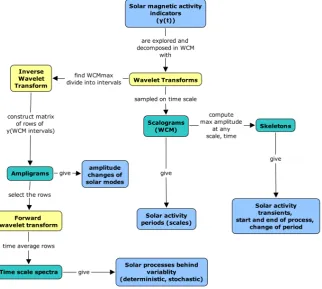
Fig. 2. The set of developed wavelet methods described in Lundstedt et al. (2005).
and Foufoula-Georgiou (1997), Torrence and Compo (1998) and Addison (2002). Wavelet analysis is a powerful tool both to find the dominant mode of variation and also to study how it varies with time, by decomposing a nonlinear time series into time-frequency space.
When the Wavelet Coefficient Magnitudes (WCM) are plotted for the scale and the elapsed time, a so-called scalo-gram is produced. Skeleton spectrum (Polygiannakis et al., 2003) can be derived from scalograms. The scale max-imal wavelet skeleton spectrum keeps only those wavelet components which are locally of maximum amplitude at any given time scale. The instantly maximal wavelet skeleton spectrum keeps only those wavelet components which are lo-cally of maximum amplitude at any given time.
In an ampligram matrix each row is the inverse wavelet transform for intervals of the maximum WCM value. It is a kind of band-pass filtering in the Wavelet Coefficient Mag-nitude domain. A Time Scale Spectra (TSS) is then derived if each row of the ampligram is wavelet-forward transformed and then time averaged.
This set of wavelet methods developed by Liszka (2003) and Wernik et al. (1997), and applied in Lundstedt et al. (2005) is summarized in Fig. 2.
Finally, Multi-Resolution Analysis (MRA) is also carried out. The idea behind MRA is to separate the information to
be analyzed into a “principal” (low pass) and a “residual” (high pass) part. The process of decomposition can then be applied again to both parts. Simplified mathematically (Mal-lat, 1998) it can be described by the following equations:
s=AJ +
X
j≤J
Dj, (1)
wheresis the signal,AJthe approximation (principal part) at
resolution levelJ andDj the detail (residual part) at level j.
From the previous formula, it is seen that the approximations are related to one another by:
AJ−1=AJ +DJ (2)
Dj =
X
k∈Z
C(j, k)9j,k(t ) , (3)
whereDj is the detail at level j,C(j, k)the wavelet
coeffi-cient and9j,k(t )the wavelet function. The wavelet used in
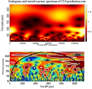
Fig. 3. Shows a scalogram and a wavelet power spectrum of the14C production rate from 9950 BC to 1950.
Fig. 4. Scalogram of the group sunspot number (to the left) and of the14C production rate (to the right).
4 Periodicities in 14C production rate longer than 22 years
A scalogram of the 14C production rate for the period –9950 BC to 1950 AD is shown in upper panel of Fig. 3. Many periodicities are apparent: the 200-year cycle (de Vries cycle), 400–500 years, 900–1000 years and 2300–2500 years (Hallstatt cycle).
We also applied the well-known wavelet tools, developed by Torrence and Compo (1998), in order to compare with statistics. The wavelet power spectrum in the lower panel of Fig. 3 shows the contours enclosing regions of greater than 90% confidence level and the cone avoidance.
1500 1600 1700 1800 1900 2000 0
0.5
1
1.5
The C14 production rate
1550 1600 1650 1700
0.8
1
1.2
1.4
The C14 production rate +/− sigma
1500 1600 1700 1800 1900 2000 0.5
1
1.5
Approximation level 4
1600 1620 1640 1660 1680 1700 1720 1740 1760 −0.1
0
0.1
Detail level 4
1500 1600 1700 1800 1900 2000 0.5
1
1.5
Approximation level 3
1600 1620 1640 1660 1680 1700 1720 1740 1760 −0.2
0
0.2
0.4
Detail level 3
1500 1600 1700 1800 1900 2000 0
0.5
1
1.5
Approximation level 2
1500 1600 1700 1800 1900 2000 −0.1
0
0.1
Detail level 2
1500 1600 1700 1800 1900 2000 0
0.5
1
1.5
Approximation level 1
1500 1600 1700 1800 1900 2000 −0.05
0
0.05
[image:5.595.124.483.79.409.2]Detail level 1
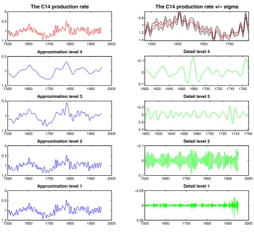
Fig. 5. Multi-resolution analysis of the14C production rate. The 22-year cycle is clearly present during the Maunder Minimum (zoomed in period) at detail level 4. The 11-year cycle is clearly present during the Maunder Minimum (zoomed in period) at detail level 3.
scales shorter than 500 years are very similar and most prob-ably due to the Sun, also before 7000 BC. However, the regions of power with greater than 90% confidence are rather localised and might therefore be related to the dropouts seen in Fig. 1. This will be further studied.
5 Cyclicity during Maunder Minimum and peaks of so-lar activity
In Fig. 1 we notice the interesting difference between the group sunspot number and the14C production rate during the Maunder minimum. The group sunspot number shows almost no activity. However, the14C production rate shows solar modulation. Similar results were obtained for10Be by Beer et al. (1998).
The scalogram of the group sunspot number is shown to the left in Fig. 4. The scalogram of the 14C production rate is shown to the right in Fig. 4. The main 11-year solar
cycle is clearly seen in both scalograms. However, the differ-ences are also obvious, especially during the Maunder min-imum. When the sunspot number shows almost no activity, then, however, the14C production rate shows solar modula-tion. This was explained in Beer et al. (1998) where during the Maunder minimum, strong toroidal magnetic flux tubes (sunspots) were absent but weak ephemeral magnetic field (also indicated by the14C production rate) were present.
16000 1700 1800 1900 2000 50
100
16000 1700 1800 1900 2000
50 100
16000 1700 1800 1900 2000
50 100 150
Approximation level 4
1600 1650 1700 1750
−50 0 50
Detail level 4
16000 1700 1800 1900 2000
50 100 150
Approximation level 3
1640 1660 1680 1700 1720
−10 0 10
Detail level 3
16000 1700 1800 1900 2000
50 100 150
Approximation level 2
1600 1700 1800 1900 2000
−50 0 50
Detail level 2
16000 1700 1800 1900 2000
50 100 150
Approximation level 1
1600 1700 1800 1900 2000
−50 0 50
[image:6.595.125.478.87.442.2]Detail level 1
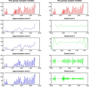
Fig. 6. Multi-resolution analysis of the group sunspot number. The 11-year cycle is not present during the Maunder Minimum (zoomed in
period) at detail level 3.
6 Transient event in late 1700
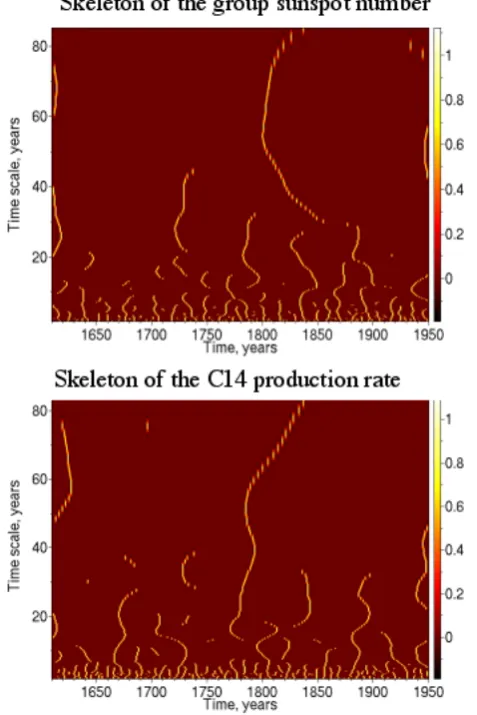
The three diagrams (Figs. 4, 7, 8) show a process starting or ending around 1750–1800. We are not aware that any solar explanation of this feature has been given. In Fig. 7 we have carried out a unit-variance filtering for the 14C production rate, i.e. we normalized the scalogram matrix with the stan-dard deviation for each dilation. The feature clearly stands out.
Skeleton can be used to discover transients, the start and end of processes and how scales change with time (Polygian-nakis et al., 2003). The scale maximal wavelet skeleton spec-trum keeps only those wavelet components that are locally of maximum amplitude at any given time scale. The instantly maximal wavelet skeleton spectrum keeps only those wavelet components that are locally of maximum amplitude at any given time.
The scale maximal skeletons to the left in Fig. 8 show the newly-discovered feature. It seems to start or end at about the end of 1700. It is interesting that the feature appears both in the group sunspot number (even if not as strong) and in the
14C production rate data. This may suggest that the feature
has a solar origin.
7 The next solar cycle and long-term trend
Figure 9 shows an ampligram of the group sunspot number (1610–1950) and the sunspot number 1995–2005.
Fig. 7. Unit-variance filtered scalogram of the14C production rate from 1500–1950.
Fig. 8. Skeletons of the group sunspot number and of the14C pro-duction rate.
Fig. 9. Ampligram of the group sunspot number 1610–1995 and the sunspot number 1995–2005. In the lower panel only the weak signal, below 20% of WCM maximum, is shown.
the weaker. The very weak components below 20% (lower panel) interestingly show some semiperiodic structure, even if they are noisier.
If the decreasing trend holds, then we would expect a weak solar cycle 24. Scientists have already predicted the ampli-tude of the next solar cycle 24: Badalyan et al. (2001) pre-dict a weak maximum, Svalgaard et al. (2005)Rz=75±10,
Duhau (2003)Rz=87.5±23.5, Kane (2002)Rz=105,
Schat-ten (2002)Rz=100±30 and Hathaway et al. (2003) predict a
large maximum.
Most expect a rather small cycle 24, i.e. in accordance with the trend. However, Hathaway et al. (2003) claim that cy-cle 24 will become strong because the meridional circulation for cycle 22 was fast.
8 Processes behind variability and interpretation
[image:7.595.48.287.296.654.2]Fig. 10. Time scale spectra, WCM (%) vs. time scales of MWSI (left) and MPSI (right) for 1975–2002 (upper panel) and time scale spectra
of the group sunspot number and the14C production rate from 1610–1950 (lower panel). BP stands for Before Present 1950.
Introducing random phase variations, but without changing the signal amplitude will broaden the dot in the horizontal direction. On the other hand, introducing random amplitude fluctuations, without scrambling the phase, will broaden the dot in the vertical direction.
In Fig. 10 (upper panel) we show time scale spectra of the solar activity indicators, MPSI and MWSI, based on mag-netic field observations for the period 1975 to 2002. The time-scale spectrum of the Mount Wilson sunspot solar mag-netic field index (MWSI) (upper left) shows mostly a feature at 11 years. The time-scale spectrum of the Mount Wilson sunspot field (MPSI) (upper right) shows, on the other hand, many additional features at 11 years. It’s interesting to notice that at least two 11-year cycles are seen as separate features, one centered at somewhat shorter time scales but stronger than the other. We also notice extended weaker features at (WCM≈40%) and (WCM≈20%).
In the lower panel of Fig. 10 the TSS of the group sunspot number and the14C production rate are shown for the scale 2–14 years, in order to emphasize the main 11-year cycle in the two data sets. In TSS of the group sunspot number the main 11-year cycle is distinct and clear. In the TSS of the
14C production rate there seems to be two processes.
Solar magnetograms are clearly the best indicators of so-lar activity to explore. They reveal many features, which are more directly related to solar phenomena. In Boberg et al. (2002) we studied the solar mean magnetic field, derived from magnetograms observed at Wicox Solar Observatory (Scherrer et al., 1977) and SOHO, in order to investigate so-lar activity on shorter terms of two years and less.
9 Conclusions and discussions
activity we used the14C production rate, the group sunspot number and the sunspot number. We used Mt. Wilson mag-netic field data for comparisons, i.e. more physics-based data.
Scalograms, skeletons, ampligrams and time scale spec-tra were presented for the long-term solar activity indicators. We also carried out MRA. By applying these methods we were able to show both similarities and differences between the data sets. The14C production rate data showed an inter-esting variability during the Maunder minimum. We found many different periodicities and showed how they changed with time. We found a new solar activity feature around the end of 1700, not earlier described. We showed both deter-ministic and more stochastic features in the variability of the indicators.
The solar activity indicator 14C production rate showed several interesting features: peaks of solar activity not seen in the group sunspot number, and variability at the 22- and 11-year cycle during the Maunder minimum. A transient event in late 1700 also appeared in the group sunspot number but not as strong. There were more deterministic processes be-hind the variability than for the group sunspot number. Since it appears that the14C production rate is a proxy of both the weak and the strong solar magnetic field variability, it is very important to understand all the processes behind the variabil-ity of the14C production rate. If this can be achieved, then the14C production rate might become a very important indi-cator of long-term solar magnetic activity.
However, when solar magnetic field observations (Schri-jver and Zwaan, 2000) are available they are preferred as indicators of the solar activity. A new picture of the Sun’s activity is also emerging, based on observations of all time and spatial scales of the solar magnetic field variability (Ti-tle, 2005). MRAs are very suitable for analysing that vari-ability. In an upcoming article, such a study is carried out of the averaged synoptic magnetic fields. As soon as data is available from Solar Dynamics Observatory (SDO), then MRA will give a very interesting picture of the solar mag-netic activity. At that time we also plan study how this pic-ture is related to the picpic-ture of the long-term solar activity, as seen in MRA.
Acknowledgements. This work is sponsored by the Swedish
Na-tional Space Board. We are grateful to the following providers of data: ESA/NASA SOHO/MDI team, Wilcox Solar Observatory, Stanford, Mount Wilson Observatory, UCLA, RWC Belgium, Hoyt and Schatten for Rg, NOAA and SEC.
Topical Editor B. Forsyth thanks L. Svalgaard and E. Lucek for their help in evaluating this paper.
References
Addison, P.: The Illustrated Wavelet Transform Handbook, In-troductory Theory and Applications in Science, Engineering, Medicine and Finance, Institute of Physics Publishing, Bristol, 2002.
Badalyan, O., Obridko, V., and Sykora, N. J.: Brightness of the coronal green line and prediction for activity cycles 23 and 24, Solar Physics, 199, 421–435, 2001.
Beer, J., Tobias, S., and Weiss, N.: An Active Sun Throughout the Maunder Minimum, Solar Phys., 181, 237–249, 1998.
Boberg, F., Lundstedt, H., Hoeksema, J. T., Scherrer, P. H., and Lui, W.: Solar mean magnetic field variability: A wavelet approach to WSO and SOHO/MDI observations, J. Geophys. Res., Vol. 107, No A10, 15-1–15-7, 2002.
Christensen-Dalsgaard J. and Thompson, M. J.: Rotation of the so-lar interior, edited by: Dwivedi, B. N., Dynamic Sun, 2003. Dikpati, M. and Charbonneau, P.: A Babcock-Leighton flux
trans-port dynamo with solar-like differential rotation, Astrophys. J., 518, 508–520, 1999.
Duhau, S.: An Early Prediction of Maximum Sunspot Number in Solar Cycle 24, Solar Physics, 213 (1), 203–212, 2003. Fu, L.-M.: Neural Networks in Computer Intelligence, McGraw-Ill,
Inc., 1994.
Hathaway, D. H., Nandy, D., Wilson, R. M., and Reichmann, E. J.: Evidence that Deep Meridional Flow Sets the Sunspot Cycle Period, Astrophys. J., 589, 665–670, 2003.
Hoyt, D. V. and Schatten, K.: Group Sunspot Numbers: A New So-lar Activity Reconstruction, SoSo-lar Physics, 181, 491–512, 1998. Jensen, J. M., Lundstedt, H., Thompson, M. J., Pijpers, F. P., and
Rajaguru, S. P.: Application of Local-Area Helioseismic Meth-ods as Predicters of Space Weather, in Helio- and Asteroseis-mology: Towards a Golden Future, edited by: Danesy, D., Proc. SOHO 14/GONG+ 2004 Meeting, ESA SP-559, 497–500, 2004. Kane, R. P.: Prediction of solar activity: Role of long-term
varia-tions, J. Geophys Res., 107, 3-1–3-3, 2002.
Kumar, P. and Foufoula-Georgiou, E.: Wavelet analysis for geo-physical applications, Rev. Geophys. 35(4), 385–412, 1997. Liszka, L.: Cognitive Information Processing in Space Physics and
Astrophysics, Pachart Publishing House, Tuscon, 2003. Lundstedt, H.: Solar Activity Predicted with Artificial Intelligence,
Space Weather Geophysical Monograph, 125, AGU, 2001. Lundstedt, H.: Progress in space weather predictions and
applica-tions, Adv. Space Res., 36, 2516–2523, 2005.
Lundstedt, H.: Solar Activity Modelled and Forecasted: A New Approach, (presented at COSPAR meeting in Paris 2004), Adv. Space Res., in press, 2006.
Lundstedt, H., Liszka, L., and Lundin, R.: Solar activity explored with new wavelet methods, Ann. Geophys., 23, 1505–1511, 2005,
SRef-ID: 1432-0576/ag/2005-23-1505.
Mallat, S.: A wavelet tour of signal processing, Academic Press, 1998.
Muscheler, R., Beer, J., and Kubik, P. W.: Long-Term Solar Vari-ability and Climate Change Based on Radionuclide Data From Ice Cores, in: Solar Variability and its Effect on the Earth’s At-mospheric and Climate System, edited by: Pap, J. P. F., AGU Geophysical Monograph series, 221–235, 2004.
Muscheler, R., Joos, F., Muller, S. A., and Snowball, I.: Climate: How unusual is today’s solar activity?, Brief Communications Arising, Nature, 436, E4–E5, 2005a.
Schatten, K.: Solar activity prediction: Timing predictors and cy-cle 24, J. Geophys., Res., 107, 15-1–15-7, 2002.
Scherrer, P. H., Wilcox, J. M., Svalgaard, L., Duvall, T. L., Dittmer, P. H., and Gustafson, E. K.: The mean magnetic field of the sun: Observations at Stanford, Solar Physics, 54, 353–361, 1977. Schlesinger, M. and Andronova, N. G.: Has the Sun Changed
Cli-mate? Modeling the Effect of Solar Variability on Climate, in: Solar Variability and its Effect on Climate, edited by: Pap, J. M. and Fox, P., Geophys. Monograph, 141, 261–282, 2003.
doi:10.1029/2004GL021664, 2005.
Title, A.: Toward Understanding the Sun’s Magnetic Fields and Their Effects, EGU General Assembly 2004, Geophys. Res. Ab-str., vol. 6, 2004.
Torrence, C. and Compo, G. P.: A practical guide to wavelet analy-sis, Bull. Am. Meteorol. Soc., 79, 61–78, 1998.