Output-feedback co-ordinated decentralized adaptive tracking: The case of MIMO subsystems with delayed interconnections

Published online 23 May 2005 in Wiley InterScience (www.interscience.wiley.com) DOI:10.1002/acs.875

Output-feedback co-ordinated decentralized adaptive

tracking: The case of MIMO subsystems with

delayed interconnections

Boris M. Mirkin

_{and Per-Olof Gutman}

Faculty of Civil and Environmental Engineering, The Division of Environmental, Water and Agricultural Engineering, Technion}Israel Institute of Technology, Haifa 32000, Israel

SUMMARY

Exact decentralized output-feedback Lyapunov-based designs of direct model reference adaptive control (MRAC) for linear interconnected delay systems with MIMO subsystems are introduced. The design process uses a co-ordinated decentralized structure of adaptive control with reference model co-ordination which requires an exchange of signals between the different reference models. It is shown that in the framework of the reference model co-ordination zero residual tracking error is possible, exactly as in the case with SISO subsystems. We develop decentralized MRAC on the base ofa prioriinformation about only the local subsystems gain frequency matrices without additional a prioriknowledge about the full system gain frequency matrix. To achieve a better adaptation performance we propose proportional, integral time-delayed adaptation laws. The appropriate Lyapunov–Krasovskii type functional is suggested to design the update mechanism for the controller parameters, and in order to prove stability. Two different adaptive DMRAC schemes are proposed, being the first asymptotic exact zero tracking results for linear interconnected delay systems with MIMO subsystems. Copyright#2005 John Wiley & Sons, Ltd.

KEY WORDS: adaptive control; decentralized control; time-delay systems

1. INTRODUCTION

An increasing number of control problems for composite interconnected systems requires the use of an adaptive decentralized control structure with physically distributed controllers. These problems are found in various application areas, such as large-scale computer networks, power systems, automotive systems, web handling systems, etc. Also time delays are commonly encountered in various engineering systems. Decentralized control schemes present a practical and efficient means for designing control algorithms which are based only on local information while computer networks provide an infrastructure for their realization. In the case of

Contract/grant sponsor: Israel Science Foundation; contract/grant number: 38/03 Contract/grant sponsor: Centre for Absorption in Science

Received 1 September 2004 Accepted 18 February 2005 Copyright#_{2005 John Wiley & Sons, Ltd.}

y_{E-mail: [email protected]}

n

non-delayed plants with single-input single-output (SISO) interconnected subsystems, these problems are extensively studied and many important results have been obtained. The design has been based mainly on the following approaches: the traditional certainty equivalence approach or Morse’s ‘dynamic certainty equivalence approach’ (see, e.g. the books [1, 2] and the papers [3–9]), and the non-linear design tool of Krstic´, Kanellakopoulos and Kokotovic´, based on recursive backstepping and tuning function techniques (see, e.g. References [10, 11]). Extensive literature references can be found in the survey paper [12] and in the papers quoted above.

Less attention has been paid to the decentralized adaptive control problem for composite systems with time delays. For large scale systems with time-varying delays in the interconnections, linear and non-linear stabilization algorithms were proposed in Reference [13]. Robust decentralized stabilization with state feedback was considered in Reference [14]. The problem of robust state stabilization of a class of time-varying large scale systems subject to non-linear inputs, external disturbances, uncertain parameters and multiple time-varying delays in the interconnections was considered in Reference [15]. More recently, theH1 _output feedback stabilization problem, the non-fragile decentralized controller design problem, and the model following variable structure problem in the framework of systems with state time delays was considered in References [16–18], respectively.

Decentralized model reference adaptive control (DMRAC) problems for state delay systems was treated in Reference [19], wherestate feedback decentralized adaptive control with model co-ordination was considered. For composite linear delay systems with SISO interconnected subsystems a new decentralized information structure of adaptive control with reference model co-ordination was developed in our contribution [20]. In that paper, output feedback

decentralized control of state delay systems was proposed that made use of co-ordinating information about reference signals of the other subsystems in all local control laws, see also e.g. Reference [9]. This structure which is based on using a ‘dynamic co-ordinated adaptive feedforward’ in the framework of model reference decentralized output feedback adaptive control with model co-ordination guarantees zero residual tracking error.

However, these results do not appear to be easily applied to the case of composite systems with state delays and with multi-input multi-output (MIMO) subsystems. One reason for this is that the type of a prioriinformation pertaining to the overall MIMO plant structure is not as apparent in the case of MIMO subsystems as it is in the SISO case.

One of the main difficulties of this case, even without the requirement of a decentralized control structure, is the generalization of the high frequency gain sign condition, since we deal with matrix gains instead of scalar gains. Current MIMO adaptive control algorithms for systems without a decentralized control structure require somea prioriknowledge or constraints on the high-frequency gain matrix Kp¼lims!sWðsÞ of the overall plant (controlled object)

WðsÞ:The matrixKp plays a roˆle in the MIMO context of centralized adaptive control which is

analogous to that of the high frequency gain sign in SISO adaptive control [21]. A priori

knowledge of the high frequency matrix of the overall plant is critical for the design of adaptive algorithms. Most available results assume that either the high frequency matrix of the overall plant is known fully or partially, see, e.g. Reference [21], or satisfies some positive definiteness condition, i.e. the knowledge of a non-singular matrixSpsuch thatKpSp¼ ðKpSpÞT40;see, e.g.

Reference [22]. To reduce the amount ofa priorirequirements to execute the design, some recent solutions based on Morse’s factorizations ofKpwere suggested. See, e.g. the recent monograph

We postulate that the controller is decentralized which creates information constraints in the sense that the output vector yiðtÞ of the subsystem i is available as a measurement only for

controlleri;and not for the other controllers. These pose control design difficulties in addition to those caused by the presence of the time delays. As a consequence, additional demands will appear on the amount ofa prioriinformation about the overall plant gain frequency matrix. The adaptive control problem becomes more complex in the decentralized case, and is yet anunsolved problem.

To the authors’ knowledge, results for composite systems with MIMO subsystems have not been reported in the literature, even for large-scale systems without delays in the interconnections.

Our concept of reference model co-ordination [9, 20] and recent advances in output feedback design for MIMO centralized systems, e.g. References [23–25] provide tools to overcome the difficulties caused by the lack of a priori information. We develop an adaptive decentralized control parametrization for the class of composite delayed linear systems with MIMO subsystems which admits output decentralized model reference adaptive designs with zero asymptotical errors on the basis of some a prioriknowledge about the subsystem matricesKpi;but without

a prioriknowledge about the full matrixKp:Thus this paper generalizes the results in Reference

[20] to a class of linear large-scale systems with MIMO subsystems and delayed communications.

2. PROBLEM STATEMENT

We consider a class of uncertain systems, which are composed ofM multi-input ðuiðtÞÞ

multi-output ðyiðtÞÞ subsystems with delayed interconnections described by equations, suitably

initialized, of the form

yiðtÞ ¼WiðsÞ½uiðtÞ þ

XM

j¼1;j=i

WijðsÞ½yjðtÞ ð1Þ

fori¼1;2;. . .;M;where for theith subsystem,uiðtÞ 2Rmi is the control input vector,yiðtÞ 2Rmi is

the output vector, andWiðsÞ ¼CiðsIAiÞ1Biis anmimistrictly proper transfer function matrix

with uncertain parameters and with s being the Laplace transform variable or the differentia-tion operator as the case may be. The delayed interconnecdifferentia-tion is expressed by letting WijðsÞ ¼

WiðsÞA

n

ijestij;whereA

n

ij 2R

mimj _{have unknown elements andt}

ij 2Rþ are known time delays.

We make the following assumptions: (A1) the observability indexniofWiðsÞis known; (A2)

the transmission zeros of WiðsÞ have negative real parts (minimum phase plants); (A3) the

plant has full rank and vector relative degree 1. For the high frequency gain matrix

Kpi¼lims!1sWiðsÞ we assume that, in case 1: (A4) there exists a matrix Spi such that

KpiSpi¼ ðKpiSpiÞT>0 or that, in case 2:ðA40Þ the signs of the high frequency gain matrixKpi

leading principal minors are known.

Remark 1

Assumptions (A1)–(A4) are independent of the decentralized MRAC problem. They are well understood in centralized adaptive control literature and various techniques for their relaxation are known, see, e.g. the textbooks [22, 23].

Our control objective is to achieve that yi asymptotically exact follows the output yri of

a stable reference model whereby the reference model is without time-delay. Because of

assumption (A3), without loss of generality, we select theMdiagonal SPR reference models for theM subsystems as

yri¼WriðsÞri

WriðsÞ ¼diag½ðsþar1Þ. . .ðsþarMÞ1

ð2Þ

where ari>0; i¼1;. . .;M: The reference signal riðtÞ is assumed piecewise continuous and

uniformly bounded.

3. PROPOSED CONTROLLER STRUCTURE AND BASE ERROR EQUATION: KNOWN PARAMETERS

As in Reference [20] for the SISO case, we will use the Lyapunov framework to derive DMRAC for the MIMO case. The design procedure is then similar to the one used in the SISO case. As usual in adaptive control theory, it will include: (1) finding a controller structure that is based only on accessible signals, and admits perfect output tracking; (2) deriving the error equation; (3) finding a Lyapunov–Krasovskii functional and use it to derive parameter updating laws such that the error will tend to zero.

3.1. Controller structure

We postulate that the controller is decentralized, i.e. the feedback part ofuiis based only on the local

signals yi; ui: Motivated by the similarities with the SISO case [20], we will use the decentralized

adaptive control scheme withreference model co-ordinationto achieve the control objective }asymp-totic exact tracking.The control law for theith local MIMO subsystemuiis chosen to be of the form

uiðtÞ ¼uliðtÞ þuciðtÞ ð3Þ

where the part of the control lawuliðtÞis based only on the local signals of theith subsystem, and

the componentuciðtÞis the co-ordinated component which is based on the reference signals of

the all other subsystems. Exchange of the reference signals between subsystems can be easily implemented in real-life control systems.

Remark 2

For the case of systems with MIMO interconnected subsystems, the main difficulties and the main difference from the case with SISO interconnected subsystems is the choice of a suitable parametrization of the local and co-ordinated component of the control law (3), in order to anticipate the future effect of the cross-coupling. The component based on local signals,uliðtÞ;will be

modified in comparison with Reference [20] by adding a term based on local data. As the basic building block for the co-ordinated componentuciðtÞ;we suggest a dynamical system (pre-filter) with

adjustable parameters that describes how the reference signalrjðtÞof thejth reference model acts on

theith control input. As we will see below, the structure of ordinated part of the control law co-ordinated part does not depend on the particular type of thea prioriknowledge about the subsystem high frequency gain matrices,Kpi:Different types ofa prioriknowledge aboutKpi will change only

the local part of control law. We consider two extreme cases ofa priori knowledge aboutKpi: the

‘classical’ case withKpisatisfying some positive definiteness condition, see, e.g. Reference [22], and the

3.1.1. Control component based only on local information. The part of the control lawuliwhich

is based only on the local information is parameterized as follows:

uliðtÞ ¼y

nT

li oliðtÞ ¼y

nT

fi ofiðtÞ þy

nT

i oiðtÞ ð4Þ

where yn

li¼ ½y

nT

fi y

nT

i T2R

miðniþ3Þmi_;yn

fi ¼ ½y

n

ei y

nT 1i y

nT 2iT2R

miðniþ1Þmi_{; y}n

ei2R

mimi_{; y}n

1i; y

n

2i2

Rmiðni1Þmi _{and y}n

i ¼ ½y

n

r1i y

n

r2i

T_2R2mimi_{; y}n

r1i;y

n

r2i2R

mimi _{are some constant parameter} matrices,ofiðtÞandoiðtÞare the local feedback and the local feedforward signals, respectively,

and are given by the following equation ði;j¼1;. . .;MÞ:

ofiðtÞ ¼

Imi 0 0 0 FiðsÞ 0

0 0 FiðsÞ

2 6 6 4 3 7 7 5 ei yi ui 2 6 6 4 3 7 7 5ðtÞ

oiðtÞ ¼

Imi

WriðsÞ

" #

½riðtÞ ð5Þ

with

FiðsÞ ¼

½Imis

ni2_{;. . .;I}

mis;Imi

T

LiðsÞ

ð6Þ

FiðsÞ 2Rmiðni1Þmi; Imi 2R

mimi _{is an identity matrix and L}

iðsÞ ¼sni1þ þlmisþl0i is a

monic Hurwitz polynomial.

Remark 3

When comparing the control component based on local signals, uliðtÞ;of subsystem iregarded

as an isolated system, with the standard case of MIMO centralized adaptive control, one notices the following differences: In uliðtÞ the additional term y

n

r2iWriðsÞ½riðtÞ is present, and

the tracking error eiðtÞ ¼yiðtÞ yriðtÞis used in the local feedback signal vector ofiðtÞ instead

of yiðtÞ:

3.1.2. Co-ordinated control component. The co-ordinated control component, uciðtÞ; which is

based on the reference signals of the all other subsystems is chosen as follows:

uciðtÞ ¼

XM

j¼1; j=_i

ynT

ij oijðtÞ; oijðtÞ ¼PijðsÞ½rjðtÞ ð7Þ

where yn

ij¼ ½y

n_T

1ij y

n_T

2ij

T_2Rmjnimi_{; y}n

1ij2R

mjmi_{; y}n

2ij 2R

mjðni1Þmi _{are some constant parameter} matrices, andoijðtÞis the output of the dynamic system with the transfer function

PijðsÞ ¼

Imj

FijðsÞ

" #

WrjðsÞestij ð8Þ

FijðsÞ ¼

½Imjs

ni2_{;. . .;I}

mjs;Imj

T

LiðsÞ

ð9Þ

This transfer function describes how the input signal rjðtÞof thejth reference model acts on

theith control input.

The state space representation of the co-ordinated control component can be written as

uciðtÞ ¼

XM

j¼1; j=i

ynT

ij oijðtÞ

’

ZrijðtÞ ¼AfijZrijðtÞ þBfijyrjðttijÞ

zrijðtÞ ¼CfijZrijðtÞ

oijðtÞ ¼ ½zTrijðtÞyTrjðttijÞT ð10Þ

where the tripleðAfij;Bfij;CfijÞis a minimal state space realization for the stable transfer matrix

FijðsÞfrom (9).

3.2. Basic error equation

To develop an adaptation law for the controller (3)–(7), we need to express the closed-loop system in terms of the tracking erroreiðtÞ ¼yiðtÞ yriðtÞ:

With the specification ofLiðsÞ;FiðsÞandWiðsÞin the local control component (4) there exist

some constant matricesyn

ri¼Kpi1;y

n

ei;y

n

1i andy

n

2i [21, 22] such that

yn

r1iWri1ðsÞWiðsÞ ¼Iy

n_T

ei FiðsÞ y

n_T

1i FiðsÞWiðsÞ y

n

2iWiðsÞ ð11Þ

Then from (1) and (11), for any ui we have the following equation for the tracking error

ei¼yiyri;with:

ei¼WriðsÞKpi uiy

n

eiyiy

nT

1i FiðsÞyiy

nT

2iFiðsÞuiy

n

r1iriþ

XM

j¼1;j=i

An

ijyjðttijÞ

"

X

M

j¼1;j=_i

yn_T

2iFiðsÞ½A

n

ijyjðttijÞ

#

ð12Þ

Denotingz An

zij¼ ½y

n1T 1i A

n

ij;y

n2T 1i A

n

ij;. . .;y

nðni1ÞT 1i A

n

ij; A

n

zij2R

mimjðni1Þ

; using (6) and (9) and doing some manipulations with the transfer functions we can write

yn_T

2iFiðsÞA

n

ij¼A

n

zijFijðsÞ ð13Þ

In view of (13) and (5) after substitutingyj ¼ejþyrjin the right part of (12), the last equation

can be rewritten as

ei¼WriðsÞKpi uiy

n_T

fi ofiðtÞ y

n_T

i oiðtÞ þ

XM

j¼1; j=_i

½An

ij; A

n

zij

Imj

FijðsÞ

" #

WrjðsÞestij½rjðtÞ

"

þ X

M

j¼1; j=_i

ðAn

ijejðttijÞ A

n

zijFijðsÞ½ejðttijÞÞ

#

ð14Þ

z

Caveat for notation. We will use in this paper a subscript to denote a different vector, e.g.xiand a superscript to denote the ‘k’ element of this vector, e.g.xk

Finally, using (4), (7)–(10) the basic tracking error equation (14) can be expressed as

ei¼WriðsÞKpi uiy

n_T

li oliðtÞ

XM

j¼1;j=_i

yn_T

ij oijðtÞ

"

þ X

M

j¼1;j=i

ðAn

ijejðttijÞ A

n

zijFijðsÞ½ejðttijÞÞ

#

ð15Þ

whereoliðtÞ ¼ ½ofiðtÞ oiðtÞT is the ‘local regressor’ vector andy

n

ij¼ ½A

n_T

ij ;A

n_T

zijT:

4. ADAPTIVE CONTROLLER 1

First we will develop the decentralized controller under the assumption (A4), see, e.g. [22].

4.1. Control law and error equation

As the adaptive version of (3)–(7), we will use a control law of the same form as in (3), (4) and (7) but with time-varying parameter matricesyliðtÞandyijðtÞinstead of the unknown parameter

matrices yn

li andy

n

ij

uiðtÞ ¼yTliðtÞoliðtÞ þ

XM

j¼1; j=i

yT_ijðtÞoijðtÞ ð16Þ

To design update laws for the control parameter matricesyliðtÞandyijðtÞin the adaptive control

(16), we first introduce an auxiliary stable dynamic systemðAfij;Bfij;CfijÞand use (10), (16) to

write the following minimal state representation of (15):

’%

eiðtÞ ¼A%ie%iðtÞ þB%iKpi

"

*

yliðtÞoliðtÞ þ

X

j¼1; j=_i *

yijðtÞoijðtÞ

þ X

M

j¼1; j=i

ðAn

ije%jðttijÞ A

n

zijzeijðtÞÞ

#

’

ZeijðtÞ ¼AfijZeijðtÞ þBfijC%je%jðttijÞ

zeijðtÞ ¼CfijZeijðtÞ

eiðtÞ ¼yiðtÞ ymiðtÞ ¼C%ie%iðtÞ ð17Þ

wherey*liðtÞ ¼yliðtÞ y

n

li andy*ijðtÞ ¼yijðtÞ y

n

ij are parameter error matrices.

Because C%T

iðsIA%iÞ1B%i¼WmiðsÞKpi is SPR, the triple ðA%i;B%i;C%iÞ satisfies the following

equations given by the matrix version of the KY Lemma [26, p. 67]: %

AT_iP%iþP%iA%iþQ%i¼0; P%iB%i¼C%Ti ð18Þ

whereP%i¼P%Ti >0 and Q%i¼Q%i>0:SinceAfij in (10) is stable, it also hold that

AT_fijPzijþPzijAfijþQzij ¼0; i;j¼1;. . .;M ð19Þ

wherePzij ¼PTzij>0 andQzij¼QTzij>0:

4.2. Adaptation algorithms

We now choose the adaptation algorithms as ði;j¼1;. . .;MÞ

yliðtÞ ¼ Zið0Þ ZiðtÞ ZiðthiÞ

Rt

0ZiðsÞds

ZT

iðtÞ ¼giSpieiðtÞoTliðtÞ

ð20Þ

yijðtÞ ¼ Zijð0Þ ZijðtÞ ZijðthijÞ R₀tZijðsÞds

ZT

ijðtÞ ¼gijSpieiðtÞoTijðtÞ

ð21Þ

or in differential form

’

yliðtÞ ¼ ZiðtÞ Z’iðtÞ Z’iðthiÞ

ZT

iðtÞ ¼giSpieiðtÞoTliðtÞ

ð22Þ

’

yijðtÞ ¼ ZijðtÞ

ZT

ijðtÞ ¼gijSpieiðtÞoTijðtÞ

ð23Þ

Remark 4

Although only the integral component Z_iðtÞ ðZ_’iðtÞ ¼0 and Z’iðthiÞ ¼0 in (22)) of the

adaptation algorithm is needed for stability and exact asymptotic tracking, the use of the proportionalZ’iðtÞand the proportional delayedZ’iðthiÞterms in the adaptation algorithm (22)

makes it possible to achieve better adaptation performance than the traditional I and PI schemes. The idea using such a proportional, integral, time delayed (PITD) adaptation stems from Reference [27], in which a PITD adaptation algorithm is used for the centralized adaptive control of SISO plants. This adaptation algorithm includes the traditional I and PI schemes as a special case. The design parametershiandhijare chosen in the same way as the traditional gains

g_i andg_ij in (20), (22).

4.3. Stability analysis

For the stability analysis we propose the Lyapunov–Krasovskii type functional

V ¼X

M

i¼1

VeiþVZiþ

XM

j¼1; j=_i

VZijþVzijþ

Z t

ttij %

eT_jðsÞQee%jðsÞds

!

" #

Vei¼e%TiP%ie%i; Vzij ¼ZTeijPzijZeij

VZi¼

1

g_itr Z*iGiZ*

T

i þ

Z t

thi

Z_iðsÞGiZTiðsÞds

VZij¼

XM

j¼1;j=_i 1

g_ijtr Z*ijðtÞGiZ*

T

ijðtÞ þ

Z t

thij

Z_ijðsÞGiZTijðsÞds

!

where

*

Zi¼y*liðtÞ þZni þZiðtÞ þZiðthiÞ

*

Zij¼y*ijðtÞ þZijðtÞ þZijðthijÞ

ð25Þ

Qe¼QTe >0; Gi¼KpiTSpi1; the known matrix Spi satisfies KpiSpi¼ ðKpiSpiÞT>0; see (A4),

g_i>0; g_ij>0; hi>0 and hij>0 are some design parameters and Z

n

i is an as yet unspecified

positive constant vector.

Remark 5

In order to prove stability of the DMRAC scheme proposed here, some modifications with respect to Reference [20] were found necessary: we introduce auxiliary terms denoted byVZi

andVZij:

Using (18) and (19), the time derivatives of the components of (24) along (17) can be written as

’

Vei¼ %eTiðtÞQie%iðtÞ þ

XM

j¼1;j=_i

2e%T_iðtÞP%iB%iKpiA

n

ije%jðttijÞ

X

M

j¼1;j=_i

2e%T_iðtÞP%iB%iKpiA

n

zijCfijZeijðtÞ þtrðofie%TiP%iB%iKpiy*TfiÞ þtrðy*fiKpiTB%TiP%ie%ioTfiÞ

þ X

M

j¼1

trðoij%eTiP%iB%iKpiy*TijÞ þ

XM

j¼1

trðy*ijKpiTB%TiP%ie%ioTijÞ ð26Þ

’

Vzij¼

XM

j¼1; j=_i

ZT_eijðtÞQzijZeijðtÞ þ

XM

j¼1; j=_i

2Z_eijTðtÞP%zijBfijC%je%jðttijÞ ð27Þ

’

VZi¼ trð½ZiðtÞ þZiðthiÞGi½ZiðtÞ þZiðthiÞTÞ trðZiðtÞGiy*TfiðtÞ þy*fiðtÞGiZTiðtÞÞ

trðZ_iðtÞGiZi* TþZ

n

iGiZTiðtÞÞ ð28Þ

’

VZij¼ tr½ZijðtÞ þZijðthijÞGi½ZijðtÞ þZijðthijÞT

trðZ_ijðtÞGiy*TijðtÞ þy*ijðtÞGiZTijðtÞÞ ð29Þ

Let us now choose

Zn_T

i ¼ 12K

1

pi Qi0. . .0

h i

; Qi¼QTi >0 ð30Þ

Then, in view of Equations (20) and (18), we get for the last terms of (28)

trðZiðtÞGiZ

n_T

i þZ

n

iGiZTiðtÞÞ ¼e%TiP%TiB%iQiB%TiP%i%ei ð31Þ

Remark 6

This term, (31), aids the proof and does not influence the control value. It allows us to prove stability of the closed decentralized system without an additional term in the control law, as was done in, e.g. Reference [8].

Now, using (26)–(29), dropping negative terms and exploiting (20), (30) and (31), it can be shown that the time derivative of (24) along the error equation (17) is given by

’

Vjð17Þ4

XM

i¼1

_%eT_iðtÞQie%iðtÞ e%TiP%

T

iB%iQiB%TiP%ie%i

XM

j¼1; j=_i

ZT_eijðtÞQzijZeijðtÞ

"

X

M

j¼1; j=_i %

eT_jðttijÞQee%jðttijÞ þ

XM

j¼1; j=_i

2e_%T_iðtÞP%iB%iKpiA

n

ije%jðttijÞ

X

M

j¼1;j=i

2e%T_jðtÞP%iB%iKpiA

n

zijCfijZeijðtÞ þ

XM

j¼1;j=i

2ZT_eijðtÞP%zijBfijC%j%ejðttijÞ

# ð32Þ

withQi¼QTi ¼Q%iQe>0:

Using the known fact that for any vectors x;y and any positive-definite matrix Si of

appropriate dimensions, it holds that

2xy4xTSixþyTSi1y

by which we can estimate the mixed terms of (32) as follows:

2e_%T_iðtÞP%iB%iKpiA

n

ije%jðttijÞ4e%iTðtÞP%iB%iC1ijB%iTP%ie%iðtÞ þ%eTjðttijÞSie%jðttijÞ

2e_%T_iðtÞP%iB%iKpiA

n

zijCfijZeijðtÞ4e%iTðtÞP%iB%iC2ijB%iTP%ie%iðtÞ þZeijTðtÞSiZeijðtÞ

2ZT_eijðtÞP%zijBfijC%je%jðttijÞ4ZTeijðtÞSiZeijðtÞ þeTjðttijÞC3ije%jðttijÞ ð33Þ

where

C1ij¼KpiAnijSi1A

nT

ij KpiT

C2ij¼KpiA

n

zijCfijSi1CTfijA

n_T

zijKpiT

C3ij¼C%TjBTfijP%zijSi1P%zijBfijC%j

ð34Þ

Applying (33) to (32) yields

’

Vj_ð17Þ4X

M

i¼1

_%eT_iðtÞQie%iðtÞ

XM

j¼1;j=_i

Z_eijTðtÞðQzij2SiÞZeijðtÞ

D "

e_%T_iP%T_iB%i

1

M1QiC1ijC2ij

%

BT_iP%ie%iðtÞ

_%eT_jðttijÞðQeSiC3ijÞe%jðttijÞ

E#

Let us select values ofQi;Qzij andQefrom the inequalities ði;j¼1;. . .;MÞ

lminðQiÞ>ðM1ÞlmaxðC1ijþC2ijÞ

lminðQzijÞ>lmaxð2SiÞ

lminðQeÞ>2lmaxðSiþC3ijÞ ð36Þ

wherelminð.Þandlmaxð.Þare the minimum and maximum eigenvalues ofð.Þ;respectively.

Then we obtain from (35)

’

Vjð17Þ4

XM

i¼1

%

eT_iðtÞQie%iðtÞ þ

XM

j¼1; j=_i

½Z_eijTðtÞQzijZeijðtÞ þe%jTðttijÞQee%jðttijÞ

!

40 ð37Þ

This implies [28] thatV and, therefore,_%eiðtÞ;eiðtÞ;ZeijðtÞ;y*li;yliy*ij;yij2L1:The remainder of the stability analysis follows directly using the steps in Reference [22].

Remark 7

We note that the coefficient matrices Qi; Qzij and Qe are used only for analysis and do not

influence the control law. Decentralized controller gains adjust automatically to counter the non-desirable effects of delayed interconnections and parameter uncertainties.

4.4. Main section theorem

We summarize the main result of this section as

Theorem 1

Consider system (1) and the reference model (2). Suppose that assumptions (A1)–(A4) hold. Then the adaptive control (3) with update laws (20) assures that the closed loop signals are bounded and that the tracking erroreiðtÞconverges to zero asymptotically.

5. ADAPTIVE CONTROLLER 2

For this case ofa prioriknowledge aboutKpi;we will modify the local componentuliðtÞfrom (4)

by adding the special local feedback termyuiuiðtÞ;as in Reference [24] for the centralized case,

but the co-ordinated component remains the same as above.

5.1. Controller

The modified adaptive control component which is based only on the local information is parameterized on the following form, instead of (4):

uliðtÞ ¼yTfiofiðtÞ þyiToiðtÞ þyuiuiðtÞ ð38Þ

The first two terms have the same form as in (4). The coefficient matrix yui has the

specific upper triangular structure with zero diagonal element like in Reference [24] for the

centralized case, i.e.

yui ¼

0 y12_ui y13_ui . . . y1mi

ui

0 0 y23_ui . . . y2mi

ui

.. .

.. .

.. .

.. .

0 0 . . . 0 ymi1mi

ui

0 0 0 0 0

2 6 6 6 6 6 6 6 6 4

3 7 7 7 7 7 7 7 7 5

ð39Þ

This upper triangular matrix structure guarantees that the control component (38) is implementable without singularity, that is,

u1_liðtÞ ¼y1T_fi ðtÞofiðtÞ þy1Ti ðtÞoiðtÞ þ

Xmi

k¼2

y1_uikðtÞuk_iðtÞ

u2_liðtÞ ¼y2T_fi ðtÞofiðtÞ þy2Ti ðtÞoiðtÞ þ

Xmi

k¼3

y2_uikðtÞuk_iðtÞ

.. .

umi

li ðtÞ ¼y miT

fi ðtÞofiðtÞ þyimiTðtÞoiðtÞ þ0 ð40Þ

If we denote

Y1_liðtÞ ¼ ½y_fi1TðtÞy1T_i ðtÞy12_uiðtÞy_ui13ðtÞ. . .y1mi

ui ðtÞT

Y2_liðtÞ ¼ ½y_fi2TðtÞy2T_i ðtÞy23_uiðtÞy_ui24ðtÞ. . .y2mi

ui ðtÞT

.. .

Yð_limi1ÞðtÞ ¼ ½y_fiðmi1ÞTðtÞyð_imi1ÞTðtÞyðmi1Þmi

ui ðtÞ

T

Ymi

li ðtÞ ¼ ½y miT

fi ðtÞy miT

i ðtÞ

T _ð41Þ

and

O1_liðtÞ ¼ ½oT

fi oTi u2i u3i . . .u mi1

i u mi

i T

O2_liðtÞ ¼ ½oT

fi oTi u3i. . .u mi1

i u mi

i T

.. .

Omi

li ðtÞ ¼ ½oTfi oTi

T

ð42Þ

we can rewrite the local control component (38) as

uliðtÞ ¼

Y1T_li ðtÞO1_liðtÞ .. .

YmiT

li ðtÞO mi

li ðtÞ

2 6 6 6 6 4

3 7 7 7 7

As a result, the control law of each subsystem is

uiðtÞ ¼

Y1T_li ðtÞO1_liðtÞ .. .

YmiT

li ðtÞO mi

li ðtÞ

2 6 6 6 6 4

3 7 7 7 7

5þ

XM

j¼1; j=_i

yT_ijðtÞoijðtÞ ð44Þ

5.2. Adaptation algorithms

Let the adaptation algorithms beði;j¼1;. . .;MÞ

Yk_liðtÞ ¼ zk_ið0Þ zk_iðtÞ zk_iðthiÞ

Z t

0

zk_iðsÞds

zk_iðtÞ ¼gk_fisignðdiÞOklie

k

i; ðk¼1;. . .;liÞ

YijðtÞ ¼ zijð0Þ zijðtÞ zijðthijÞ

Z t

0

zijðsÞds

zT_ijðtÞ ¼signðDiÞGgieiðtÞoTijðtÞ ð45Þ

where signðDiÞ ¼diagfsignðdi1Þ;. . .;signðd li

iÞg:

In differential form we have ’

Yk_liðtÞ ¼ zk_iðtÞ z’k_iðtÞ z’k_iðthiÞ

zk_iðtÞ ¼gk_fisignðdiÞOklieki; ðk¼1;. . .;liÞ

’

YijðtÞ ¼ zijðtÞ z’ijðtÞ z’ijðthijÞ

zT_ijðtÞ ¼signðDiÞGgieiðtÞoTijðtÞ ð46Þ

5.3. Main section result

The main result of this section can be formulated as

Theorem 2

If each subsystem is defined by (1) with adaptive control law for each subsystem defined by (44) and the update laws (45)–(46), then the tracking error eiðtÞ ¼yiðtÞ yriðtÞ;where yriðtÞ is the

output of the reference model (2), for each interconnected subsystem will asymptotically converge to zero and the closed loop signals are bounded.

Proof

First by using the high-frequency gain matrix decomposition Kpi ¼SiDiUi and in view of

Uiui¼ui ðImiUiuiÞwe derive an error equation from the basic error equation (15)

ei¼WriðsÞSiDi uiy#

nT

li oliðtÞ y#

n

uiui

XM

j¼1; j=_i #

ynT

ij oijðtÞ þ

XM

j¼1;j=_i

ðA#n

ijejðttijÞ

"

A#n

zijFijðsÞ½ejðttijÞÞ

#

ð47Þ

where y#n

li¼Uiy

n

li; y#

n

ij¼Uiy

n

ij;A#

n

ij¼UiA

n

ij; A#

n

zij ¼UiA

n

ij and matrix y#

n

ui ¼ImiUi has the same specific upper triangular form as (39) with zero diagonal element

#

yn

ui¼

0 yn₁₂

ui y

n₁₃

ui . . . y

n_1mi

ui

0 0 yn23

ui . . . y

n2mi

ui .. . .. . .. . .. .

0 0 . . . 0 ynmi1mi

ui

0 0 0 0 0

2 6 6 6 6 6 6 6 6 6 6 4 3 7 7 7 7 7 7 7 7 7 7 5

ð48Þ

Then using the control law as given by (44), the tracking error equation (47) can be written as

ei¼WmiðsÞSiDi

* Y1T_li O1_li

.. .

* YmiT

li O mi li 2 6 6 6 6 4 3 7 7 7 7 5þ XM

j¼1;j=_i * YT_ijoij

0 B B B B @ 1 C C C C A þ X M

j¼1; j=_i

WmiðsÞSiDiðA#

n

ijejðttijÞ A#

n

zijzeijÞ ð49Þ

where

*

Yk_liðtÞ ¼Yk_liðtÞ Yn_k

li Y*ijðtÞ ¼YijðtÞ Y

n

ij

are the parameter errors,k¼1;2;. . .;mi;i;j¼1;. . .;M:

LetðA#i;B#i;C#iÞbe any minimal realization ofWiðsÞSithat is SPR [24], andðAfij;Bfij;CfijÞis a

minimal stable state space realization for the stable transfer matrixFijðsÞfrom (9). Then we can

get the following state space representation of (49):

’#

ei¼A#i#eiðtÞ þB#iDi

* Y1T li O 1 li .. . * YmiT

li O mi li 2 6 6 6 6 4 3 7 7 7 7 5þ XM

j¼1;j=_i * YT_gijogij

0 B B B B @ 1 C C C C A þ X M

j¼1; j=i

#

BiDiðA#

n

ijejðttijÞ A#

n

zijCfijZeijðtÞÞ

’

ZeijðtÞ ¼AfijZeijðtÞ þBfijC#je#jðttijÞ

eiðtÞ ¼yiðtÞ ymiðtÞ ¼C#ie#iðtÞ

SinceWmiðsÞSi is SPR, there exist [26, p. 67] positive definite matricesP#i andQ#i such that

#

AT_iP#iþP#iA#iþQ#i¼0; P#iB#i¼C#Ti ð51Þ

Remark 8

This Equation (51) and error equation (50) have only formal similarity with (18). In (51) and (50) we findWmiðsÞSi;but notWmiðsÞKpi:

For the stability analysis in this section we use the following Lyapunov–Krasovskii type functional:

V¼X

M

i¼1

VeiþVzi

XM

j¼1; j=i

VzijþVzijþ

Z t

ttij #

eT_jðsÞQee#jðsÞds

!

" #

Vei ¼e#TiP#ie#i; Vzij ¼ZTeijPzijZeij

Vzi¼

Xli

k¼1 ðgk

fiÞ

1_j

dij zkiTðtÞz k iðtÞ þ

Z t

thi

zk_iTðsÞzk_iðsÞds

Vzij¼

XM

j¼1; j=_i

tr z%ijðtÞGgi1D%i%zTijðtÞ þ

Z t

thij

zijðsÞGgi1D%izTijðsÞds

!

ð52Þ

where

*

zi¼y*liðtÞ þz

n

i þziðtÞ þziðthiÞ

*

zij¼y*ijðtÞ þzijðtÞ þzijðthijÞ

ð53Þ

Ggi¼GTgi>0;D%i¼diagfjdi1j. . .jdikj. . .jd mi

i jganddikare the entries ofDi:The matricesQe;Pzij

and the design parametershi andhij are the same as in (24). The ‘artificial’ vector

zn

i ¼r0ð2diÞ1½1;0;. . .;0T ð54Þ

has the same dimension as Yk_fi;andr0 is an as yet unspecified positive constant.

Using (51) and (19) the time derivatives of the components of (52) along (50) can be written as

’

Vei¼ e#TiðtÞQi#eiðtÞ þ

XM

j¼1;j=₁

2e_%T_iðtÞP%iB%iDiA#

n

ije%jðttijÞ

X

M

j¼1; j=i

2%eT_iðtÞP%iB%iDiA#

n

zijCfijZeijðtÞ þ2e#TiðtÞP#iB#iDi

* Y1T

li O

1

li

.. .

* YliT

li O li

li

2 6 6 6 6 4

3 7 7 7 7 5

þ X

M

j¼1

trðoije#TiP#iB#iDiY*TijÞ þ

XM

j¼1

trðY*ijDTiB#

T

iP#ie#ioTijÞ ð55Þ

’

Vzij ¼

XM

j¼1;j=_i

ZT_eijðtÞQzijZeijðtÞ þ

XM

j¼1; j=_i

2ZT_eijðtÞP#zijB#fijC#je#jðttijÞ ð56Þ

’

Vzi ¼

Xli

k¼1

ðgk_fiÞ1jdij 2Y*kliTz k

iðtÞ þ2z* kT

i z k iðtÞ

h

þ ðzk_iðtÞ þzk_iðthiÞÞTðzkiðtÞ þzkiðthiÞÞ

ð57Þ

’

Vzij¼ trðzijðtÞGgiD%iY*TijðtÞ þY*ijðtÞGgiD%izTijðtÞÞ ¼ jjzijðtÞ þzijðthijÞjjGgiD%i ð58Þ

In view of (54), (51) and (45) we can write

2 X

li

k¼1

ðgk_fiÞ1_jd

ijz

n_kT

i zkiðtÞ ¼ ro#eTiP#iTB#iB#TiP#ie#i ð59Þ

Further using (59), (55)–(58) and dropping negative terms we obtain

’

Vj_ð50Þ4X

M

i¼1

#eT_iðtÞQie#iðtÞ r0#eTiP#

T

iB#iB#TiP#ie#i

XM

j¼1; j=_i

ZT_eijðtÞQzijZeijðtÞ

"

X

M

j¼1; j=_i #

eT_jðttijÞQee#jðttijÞ þ

XM

j¼1; j=_i

2e#T_iðtÞP#iB#iDiA#

n

ije#jðttijÞ

X

M

j¼1; j=_i

2e#T_iðtÞP#iB#iDiA#

n

zijCfijZeijðtÞ þ

XM

j¼1; j=_i

2ZT_eijðtÞP#zijBfijC#j#ejðttijÞ

# ð60Þ

withQi¼QTi ¼Q#iQe>0:

We can estimate the mixed terms of (60) as follows:

2e#T_iðtÞP#iB#iDiA#

n

ije#jðttijÞ4#eTiðtÞP#iB#iC#1ijB#iTP#ie#iðtÞ þe#TjðttijÞSie#jðttijÞ

2e#T_iðtÞP#iB#iDiA#

n

zijCfijZeijðtÞ4#eiTðtÞP#iB#iC#2ijB#TiP#ie#iðtÞ þZTeijðtÞSiZeijðtÞ

2ZT_eijðtÞP#zijBfijC%je#jðttijÞ4ZTeijðtÞSiZeijðtÞ þe#jTðttijÞC#3ije#jðttijÞ ð61Þ

where

#

C1ij¼DiA#

n

ijSi1A#

n_T

ij DTi

#

C2ij¼DiA#nzijCfijSi1CTfijA#

n_T

zijDTi

#

C3ij¼C%TjBTfijP#zijSi1P#zijBfijC%j

Applying (61) to (60) yields

’

Vjð17Þ4

XM

i¼1

e#T_iðtÞQie#iðtÞ

XM

j¼1;j=_i

D

ZT_eijðtÞðQzij2SiÞZeijðtÞ

"

e#T_iP#T_iB#i

ro

M1C#1ijC#2ij

#

BT_iP#ie#iðtÞ

e#T_jðttijÞðQeSiC#3ijÞ#ejðttijÞ

E#

ð63Þ

Let us select values ofro;Qzij andQefrom the inequalities ði;j¼1;. . .;MÞ

ro>ðM1ÞlmaxðC#1ijþC#2ijÞ

lminðQzijÞ>lmaxð2SiÞ

lminðQeÞ>2lmaxðSiþC#3ijÞ ð64Þ

wherelminð*Þandlmaxð*Þare the minimum and maximum eigenvalues ofð*Þ;respectively.

Then, similarly to the previous section we get

’

Vjð50Þ4

XM

i¼1

#

eT_iðtÞQie#iðtÞ þ

XM

j¼1; j=_i

h

ZT_eijðtÞQzijZeijðtÞ þe#TjðttijÞQee#jðttijÞ

i!

40 ð65Þ

The remainder of the stability proof follows directly like in the previous section.

6. EXAMPLE

To illustrate the application of the proposed adaptive scheme, let us consider a plant with two subsystems described by (1) in state space form,

’

y1ðtÞ ¼ 1:0 0

0 1:0

" #

y1ðtÞ þ 1:0 2:0

3:0 1:0

" #

u1ðtÞ þ 6:0 7:0

10:0 14:0

" #

y2ðtt12Þ

’

y2ðtÞ ¼ 0:1 0

0 0:1

" #

y2ðtÞ þ 2:21 4:42

6:63 2:21

" #

u2ðtÞ þ 24:31 17:68 26:52 22:10

" #

y1ðtt21Þ

y1ð0Þ ¼y2ð0Þ ¼

0

0

" #

ð66Þ

We choose the reference model as

’

yr1ðtÞ ¼

1:0 0

0 1:0

" #

yr1ðtÞ þ

1:0 0

0 1:0

" #

r1ðtÞ

’

yr2ðtÞ ¼

0:8 0

0 0:8

" #

yr2ðtÞ þ

1:0 0

0 1:0

" #

r2ðtÞ

ð67Þ

yr1ð0Þ ¼

0

1

" #

yr2ð0Þ ¼ 1

0

" #

All parameters except the time delaysðt12¼6;t21 ¼4Þare unknown to the controller. The only

information available to the controller is the structural information given in Assumptions A1–A4. The adaptation algorithms (20) of the first controller in our simulation are

yT_liðtÞ ¼ g_iSpiPITDðeiðtÞoT_liðtÞÞ

yT_ijðtÞ ¼ g_ijSpiPITDðeiðtÞoTijðtÞÞ; i;j¼1;2

ð68Þ

where PITDð$_{Þ is the operator form for PITDðZ}

iðtÞÞ ¼kI

Rt

0ZiðsÞdsþkPZiðtÞ þkDZiðthiÞ;

where the parameter values were chosen as h1¼h2¼1; gi¼gij¼1; with oli¼ ½eiðtÞ

riðtÞ xriðtÞT;oij¼xrijðttijÞ;and

Spi¼

28:5714 57:1429

600 28:5714

" #

The input signals of the first reference model r1¼ ½r11 r12T are sine and square signals with

amplitudes 0.6 and 0.4, and frequencies 0.6 and 0.5, respectively. The input signals of the second reference model r2¼ ½r21 r22T are square and sine signals with amplitudes 0.5 and0:5;and

frequencies 0.9 and 0.5, respectively.

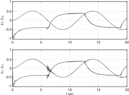
Simulation results are found in Figures 1 and 2, where the time responses of the outputs of the plantyðtÞ ¼ ½y1ðtÞ y2ðtÞT_{and the outputs of the reference modely}

rðtÞ ¼ ½yr1ðtÞ yr2ðtÞTare shown.

0 5 10 15 20

-1 -0.5 0 0.5 1

y1

, y

r1

y1

, y

r1

0 5 10 15 20

-1 -0.5 0 0.5 1

t sec

Figure 1. Simulation of the adaptive control system. The upper graphs show the time history of the subsystem 1 and reference model outputsy1ðtÞ ¼ ½y11ðtÞ y12ðtÞTandyr1ðtÞ½yr11ðtÞyr12ðtÞT;for the controller

The upper graphs in Figures 1 and 2 were generated by the plant model (66), the controller (16), with adaptation algorithms (68), and the reference model (67). The parameter valueskP

and kD are kP¼0:05 andkD¼0:005: The lower graphs show the time history with only the

-1 -0.5 0 0.5 1

y2

, y

r2

-1 -0.5 0 0.5 1

y2

, y

r2

0 5 10 15 20

0 5 10 15 20

t sec

Figure 2. Simulation of the adaptive control system. The upper graph shows the time history of the subsystem 2 and reference model outputs y2ðtÞ ¼ ½y21ðtÞ y22ðtÞT and yr2ðtÞ ¼ ½yr21ðtÞ yr22ðtÞT; for the

controller (16) and the adaptation algorithms (20). The lower graph shows the time history with only the integral part of the adaptation algorithms (68).

0 5 10 15 20 25 30 35 40 -1

-0.5 0 0.5 1

y1

, y

r1

-1 -0.5 0 0.5 1

y1

, y

r1

0 5 10 15 20 25 30 35 40 t sec

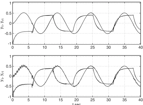
Figure 3. Simulation of the adaptive control system. The upper graph shows the time history of the subsystem 1 and reference model outputsy1ðtÞ ¼ ½y11ðtÞ y12ðtÞTandyr1ðtÞ½yr11ðtÞyr12ðtÞT;for the controller

(44) and the adaptation algorithms (45). The lower graph shows the time history with only the integral part of the adaptation algorithms (45).

integral part of the adaptation algorithms (68), i.e.kP¼kD¼0:The integral design parameter

kI ¼1 for all the simulation runs.

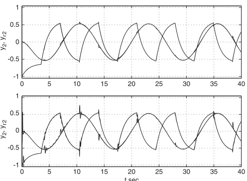
Simulation results for the second controller (44)–(46) are shown in Figures 3 and 4 with the same plant, parameters values, and reference signals as above, with the exception thatkP¼0:2

andkD¼0:002:

As expected, all signals in the system with co-ordinated decentralized controller are bounded, while stability and convergence of the errors to zero are ensured. The transient response for the controllers with PITD adaptation algorithms is better than the case when standard integral adaptation algorithms are used. The transient performance can be influenced by choosing the adaptation algorithms design parameters kI;kP; kD and h: However, as in the most existing

adaptive control schemes, there do not exist systematic analytic tuning rules. As usual in the adaptive control literature, we tuned the design parameters by trial-and-error. Our new PITD design adds the new design parameters kD and hl: Not surprisingly, we found that there is a

trade-off between transient performance and large control input variations during the transient.

7. CONCLUSION

Considering the direct certainty-equivalence DMRAC problem, we have proposed, for the first time, two parameterizations of the co-ordinated DMRAC to design output-feedback decentralized adaptive tracking control for a class of uncertain systems with MIMO subsystems and delayed communications between the subsystems. As in the case with SISO subsystems, it is shown that in the framework of reference model co-ordination zero residual tracking error is possible. The design uses decentralized local output feedback together with centralized model

-1 -0.5 0 0.5 1

y2

, y

r2

-1 -0.5 0 0.5 1

y2

, y

r2

0 5 10 15 20 25 30 35 40

0 5 10 15 20 25 30 35 40 t sec

Figure 4. Simulation of the adaptive control system. The upper graph shows the time history of the subsystem 2 and reference model outputsy2ðtÞ ¼ ½y21ðtÞ y22ðtÞT andyr2ðtÞ ¼ ½yr21ðtÞ yr22ðtÞT;for the

reference co-ordination. In this way, the totally decentralized structure of the current information update is retained, since there is no exchange of signals between the different subsystems. We developed DMRAC only on the basis of a prioriinformation about the local subsystems gain frequency matrices Kpi:We considered two cases ofa prioriknowledge about

Kpi}the ‘classical’ case withKpisatisfying some positive definiteness condition, and the recently

proposed less restrictive case based on the SDU decomposition ofKpi:In, e.g. Reference [29] an

interesting idea is presented to circumvent the need for the knowledge of the high frequency gain, for centralized SISO systems without delay. However, to the best of the authors’ knowledge, this idea has not yet found use even for centralized MIMO systems without delay, and, consequently, its extension remains an important research topic.

To achieve a better adaptation performance than traditional proportional and proportional integral adaptation algorithms, we suggested proportional, integral time-delayed adaptation laws. The appropriate Lyapunov–Krasovskii type functional is proposed to design the update mechanism for the controller parameters, and to prove stability.

As can be seen in Section 6 we can improve the transient performance of DMRAC by correspondingly choosing of the adaptive algorithms design parameters. Unfortunately, we do not have analytic tool for performance analysis. For the DMRAC with SISO subsystems and without delays there are some works (e.g. Reference [30] based on the ‘classical’ adaptive technique and Reference [31], based on the backstepping approach) where given some analytical expressions to evaluate the transient performance. These results allows us to hope that in the future it will possible to consider such problems and in the case of DMRAC with MIMO subsystems.

As can be seen in Sections 4 and 5, the developed structure of the dynamic system which forms the co-ordinate part of the control law is universal and does not depend on a priori

knowledge about the frequency gain matrices of the subsystems. Different types of a priori

information changes only the part of the control law that is based on the local signals of the subsystems. This result is pleasing, and gives hope that the present parametrization of DMRAC with its universal dynamic system structure for forming co-ordinated control signals, and recent advances in centralized MIMO adaptive control theory, e.g. the LDU, LDS decomposition of

Kp;e.g. Reference [23], and immersion and invariance MIMO adaptive control design method

[32], may provide useful tools for further designs of DMRAC with different types a priori

knowledge.

ACKNOWLEDGEMENTS

This work was supported by the Israel Science Foundation under Grant 38/03. The research of the first author was supported by the Center for Absorption in Science, Ministry of Immigrant Absorption, State of Israel.

REFERENCES

1. Ioannou PA, Kokotovic´ P.Adaptive Systems with Reduced Models.Springer: Berlin, 1983.

2. Mirkin BM, Choi M.Adaptive Decentralized Control of Dynamic Systems. Nauka: Bishkek, 1991 (in Russian). 3. Ioannou PA. Decentralized adaptive control of interconnected systems.IEEE Transactions on Automatic Control

1986;31:310–314.

4. Gavel DT, Siljak DD. Decentralized adaptive control: structural conditions for stability. IEEE Transactions on Automatic Control1989;34(4):413–426.

5. Ortega R. An energy amplification condition for decentralized adaptive stabilization. IEEE Transactions on Automatic Control1996;41:285–289.

6. Mirkin BM. Adaptive decentralized control with model coordination. Automation and Remote Control 1999; 60(1):73–81 (Translated fromAvtomatika i telemekhanika1999;1:90–100).

7. Wen C, Soh YC. Decentralized model reference adaptive control without restriction on subsystem relative degrees.

IEEE Transactions on Automatic Control1999;44(7):1464–1469.

8. Narendra KS, Oleng NO. Exact output tracking in decentralized adaptive control.IEEE Transactions on Automatic Control2002;47(2):390–395.

9. Mirkin BM. Comments on ‘Exact output tracking in decentralized adaptive control’. IEEE Transactions on Automatic Control2003;48(2):348–350.

10. Jain S, Khorrami F. Decentralized adaptive control of a class of large-scale nonlinear systems.IEEE Transactions on Automatic Control1997;42(2):136–154.

11. Jiang ZhP. Decentralized and adaptive nonlinear tracking of large-scale systems via output feedback. IEEE Transactions on Automatic Control2000;45(11):2122–2128.

12. Siljak DD. Decentralized control and computation: status and prospects. Annual Reviews in Control1996; 20: 131–141.

13. Wu H. Decentralized output feedback control of large scale interconnected time delay systems.Proceedings of the 35th Conference on Decision and Control, Kobe, Japan, 1996; 1611–1616.

14. Mahmoud MS, Bingulac S. Robust design of stabilizing controllers for interconnected time-delay systems.

Automatica1998;34:795–800.

15. Oucheriah S. Decentralized stabilization of large scale systems with multiple delays in the interconnections.

International Journal of Control2000;73(13):1213–1223.

16. Jiang B, Wang JL. Decentralized H1 _{output feedback stabilization for large-scale systems with multiple}

time-varying delays.Proceedings of the American Control Conference, Chicago, IL, 2000; 971–975.

17. Park JH. Robust nonfragile decentralized controller design for uncertain large-scale interconnected systems with time-delays.Journal of Dynamic Systems,Measurement,and Control2002;124(2):332–336.

18. Chou CH, Cheng ChCh. Decentralized model following variable structure control for perturbed large-scale systems with time-delay interconnections.Proceedings of the American Control Conference, Chicago, IL, 2000; 641–645. 19. Mirkin BM. Decentralized adaptive control with model coordination for large-scale time-delay systems.Proceedings

of the 3rd European Control Conference ECC-95, vol. 4 of 4, part 1, Rome, Italy, 1995; 2946–2950.

20. Mirkin BM, Gutman PO. Decentralized output-feedback MRAC of linear state delay systems.IEEE Transactions on Automatic Control2003;48(9):1613–1619.

21. Sastry S, Bodson M.Adaptive Control. Stability,Convergence,and Robustness. Prentice-Hall: Englewood Cliffs, NJ, 1989.

22. Ioannou PA, Sun J.Robust Adaptive Control. Prentice-Hall: Englewood Cliffs, NJ, 1996. 23. Tao G.Adaptive Control Design and Analysis. Wiley: New York, 2003.

24. Costa RR, Hsu L, Imai AK, Kokotovic´ P. Lyapunov-based adaptive control of MIMO systems.Automatica2003; 39(7):1251–1257.

25. Hsu L, Costa R, Imai AK. Multivariable adaptive control with transient overparametrization.Proceedings of the 42th IEEE Conference on Decision and Control, Hyatt Regency Maui, HI, U.S.A., 2003; 2728–2733.

26. Narendra KS, Annaswamy AM.Stable Adaptive Systems. Prentice-Hall: New York, 1989.

27. Mirkin BM. Survey of automation’s institute results in multilevel decentralized control.Problems of Automation and Control2000;1:25–34 (in Russian).

28. Hale JK, Lunel SMV.Introduction to Functional Differential Equations. Springer: New York, 1993.

29. Zhang Y, Wen C, Soh YC. Adaptive backstepping control design for systems with unknown high frequency gain.

IEEE Transactions on Automatic Control2000;45(12):2350–2354.

30. Datta A. Performance improvement in decentralized adaptive control: a modified model reference scheme.IEEE Transactions on Automatic Control1993;38:1717–1722.

31. Zhang Y, Wen C, Soh YC. Robust decentralized adaptive stabilization of interconnected systems with guaranteed transient performance.Automatica2000;36:907–915.