Role of inductive electric fields and currents in dynamical ionospheric situations

www.ann-geophys.net/25/437/2007/ © European Geosciences Union 2007

Annales

Geophysicae

Role of inductive electric fields and currents in dynamical

ionospheric situations

H. Vanham¨aki, O. Amm, and A. Viljanen

Finnish Meteorological Institute, Space Research Unit, P.O. Box 503, 00101 Helsinki, Finland

Received: 9 October 2006 – Revised: 16 January 2007 – Accepted: 8 February 2007 – Published: 8 March 2007

Abstract. We study the role of ionospheric induction in different commonly observed ionospheric situations. These include an intensifying electrojet, westward travelling surge (WTS) and-band. We use data based, realistic models for these phenomena and calculate the inductive electric fields that are created due to the temporal variations of ionospheric currents. The ionospheric induction problem is solved us-ing a new calculation technique that can handle non-uniform, time-dependent conductances and electric fields of any ge-ometry. We find that in some situations inductive effects are not negligible and the ionospheric electric field is not a pure potential field, but has a significant induced rotational part. In the WTS and-band models the induced electric field is concentrated in a small area, where the time deriva-tives are largest. In the electrojet model the induced field is significant over a large part of the jet area. In these ex-amples the induced electric field has typical values of few mV/m, which amounts to several tens of percents of the po-tential electric field present at the same locations. The in-duced electric field is associated with ionospheric and field aligned currents (FAC), that modify the overall structure of the current systems. Especially the induced FAC are often comparable to the non-inductive FAC, and may thus modify the coupling between the ionosphere and magnetosphere in the most dynamical situations. We also present some exam-ples with very simple ionospheric current systems, where the effect of different ionospheric parameters on the induction process is studied.

Keywords. Ionosphere (Electric fields and currents) – Elec-tromagnetics (Electromagnetic theory)

Correspondence to: H. Vanham¨aki

([email protected])

1 Introduction

In this paper, we study the role of inductive electric fields and currents in several common ionospheric phenomena, in-cluding an intensifying electrojet, westward travelling surge (WTS) and -band. Usually it is assumed that the iono-spheric electric field is a potential field, so that ∇×E=0, and it is well established that this is indeed the case in most situations (e.g. Untiedt and Baumjohann, 1993). However, Yoshikawa and Itonaga (1996) were the first to study how the inductive processes influence the reflection of Alfv´en waves from the ionosphere. They found that when an incident shear Alfv´en wave carrying a potential electric field is reflected from the non-isotropically conducting ionosphere, the re-flected wave consists of both shear and fast mode waves. The fast mode wave is directly related to the induced rota-tional part of the ionospheric electric field, and also the re-flected shear mode wave is modified when inductive phe-nomena are included in the analysis. Later studies by e.g. Buchert and Budnik (1997), Buchert (1998), Yoshikawa and Itonaga (2000), Lysak and Song (2001), Lysak (2004) and Sciffer et al. (2004), have confirmed these results and inves-tigated further the reflection process and the propagation of the shear and fast mode waves in the ionosphere.

knowledge there seems to be no empirical models of Alfv´en wave patterns related to some specific ionospheric events. In principle one could use a magnetospheric MHD simulation as an input in the Alfv´en wave scheme, but in practise mag-netospheric simulations use electrostatic ionospheric solvers and it would not be straightforward to couple them to an ionospheric Alfv´en wave solver (Janhunen, 1998). In addi-tion, also magnetospheric MHD simulations have problems in producing specific ionospheric phenomena.

Recently, Vanham¨aki et al. (2005) used a different ap-proach that allowed them to use purely ionospheric quanti-ties as input, instead of incident waves. They showed by approximate calculations that inductive electric fields asso-ciated with some very dynamic ionospheric phenomena, in-cluding WTS,-band and Giant Pulsation, are locally very significant. These local “hot-spots” tended to occur in those areas where the field aligned currents (FAC) were largest, so in these areas the inductive processes could well contribute to the ionosphere-magnetosphere coupling. Vanham¨aki et al. (2005) calculated the inductive fields caused by self-induction in the ionosphere (primary process) and also by the ground induced currents flowing in the conducting ground (secondary process). They concluded that at ionospheric al-titudes the secondary contribution from ground induction is always very small and smoothly distributed and in practice negligible when compared to the larger and more concen-trated primary contibution from ionospheric self-induction.

However, the calculation method used by Vanham¨aki et al. (2005) was rather approximate, giving only order of magni-tude estimates. The induced electric fields in the ionosphere were calculated as vacuum fields, i.e. the currents driven by the induced fields themselves were neglected. This approx-imation probably gives too large induced electric fields, as the effect of the neglected current should tend to decrease the induced fields according to Lenz’s law. Vanham¨aki et al. (2006) presented a new calculation method that solves the ionospheric induction problem self-consistently using only ionospheric potential electric field and conductances as in-put. This calculation method can handle non-uniform, time-dependent ionospheric conductances and electric fields of any geometry. In this paper we apply the new calculation method to several commonly observed ionospheric phenom-ena that have strong temporal variations. Our examples in-clude the previously studied WTS and-bands systems and also an intensifying electrojet. In Sects. 2–3 we briefly out-line the calculation method and discuss the general proper-ties of ionospheric induction. In Sect. 4 we present the main results for the realistic, data-based models. Section 5 is sum-mary and conclusions.

2 Theory

The calculation method has been presented by Vanham¨aki et al. (2006), and here we give just a brief summary. We use

a cartesian coordinate system where the ionospheric current sheet is taken to be the xy-plane and the z-axis points ver-tically downwards. The Earth’s magnetic field is assumed to be parallel to the z-axis, which is a reasonable approxi-mation in the northern auroral region. We also use the thin-sheet approximation, i.e. we assume that all horizontal cur-rents flow at a thin sheet at altitudez=0. We concentrate on the effects of ionospheric self-induction, so we do not include the induction effects that take place in the conducting Earth. While the ground induction has large effects on the electric and magnetic fields at the Earth’s surface, Vanham¨aki et al. (2005) concluded that at ionospheric altitudes the ground ef-fect should be negligible when compared to the efef-fects of ionospheric self-induction.

The input quantities in the calculation method presented by Vanham¨aki et al. (2006) are the 2-dimensional distribu-tions of ionospheric Pedersen and Hall conductances, 6P

and 6H, respectively, and the potential part of the

iono-spheric electric field, Epot with∇×Epot=0. The conduc-tances andEpotmay be arbitrary (yet physically reasonable) functions of time and position. In this paper we use empiri-cal models from previous data-based studies. The output of the calculation method is the induced rotational part of the electric field,Eindwith∇·Eind=0.

The potential electric field that we use as input may have been obtained from measurements or from MHD simulation by mapping the magnetospheric electric field down to the ionosphere along field lines. In principle, when we measure the ionospheric electric field we get the total field, including the induced rotational part. However, several standard anal-ysis methods such as AMIE (Richmond and Kamide, 1988), KRM, (Kamide et al., 1981) or the SuperDARN potential mapping technique (Ruohoniemi and Baker, 1998) are based on the assumption that the ionospheric electric field is a po-tential field. This assumption is also used in many data-based ionospheric models (e.g. Untiedt and Baumjohann, 1993), as well as in ionospheric solvers of magnetospheric MHD sim-ulations (e.g. Janhunen, 1998). The potential electric field obtained with any of the above techniques may be used as in-put in our calculation method, which then gives the induced rotational part of the ionospheric electric field as output.

The calculation method is based on Cartesian Elemen-tary Current Systems (CECS), that were introduced by Amm (1997). There are two kinds of elementary systems, curl-free (CF) and divergence-free (DF), which form a set of basis functions for representing 2-dimensional vector fields. The general outline of the calculation method is following:

– Express the potential (Epot) and induced rotational (Eind) parts of the electric field using CECS.

Induction

T=2

T=1 Induced E Induced Jp Induced Jh

Jh Jp

Potential E

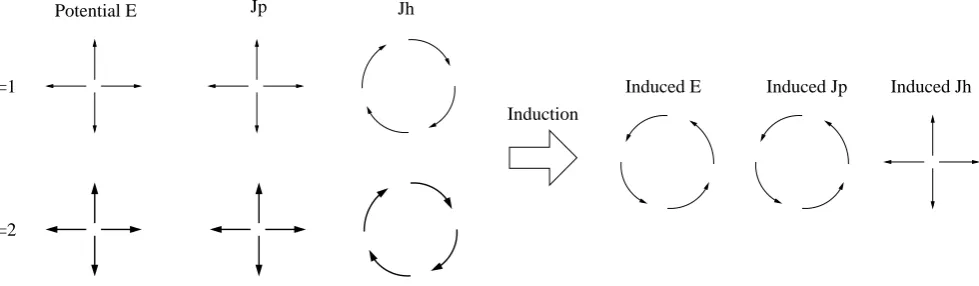
Fig. 1. Lenz’s law in the northern auroral ionosphere (with uniform conductances and downward pointing background magnetic field). Changes of the potential electric field (Epot) and associated currents (Jp and Jh) create rotational induced electric field (Eind). Induced currents oppose the change in rotational currents, but enhance the change in divergent currents (i.e. FAC).

the induced upward and downward FAC are nearly balanced. The increasingly localized nature of the induced system with smallerT is clearly visible in the|Iind_{|profiles. It seems}

that the ionospheric induction process affects the FAC more than the electric field, for the induced FAC are much larger than the input FAC, althoughEind is at most equal to in-putEpot. This is partly explained by the larger spatial scale of the induced E-field and also by the ratioΣH/ΣP = 2

of the conductances. In the input system rotational currents are Hall currents and FAC are associated with Pedersen cur-rents. In the induced system this is reversed, which means thatmax(F ACind_{/F AC1) = 4max(|E}ind_|/|Epot_|).

Figure 3 shows the effect of varying Pedersen conduc-tanceΣP, while keeping the oscillation timeTand Hall

con-ductanceΣH constant. The peak magnitude of the induced

electric field increases slightly with decreasingΣP, and the

field also decays somewhat slower with distance. This is related to the behaviour of the induced rotational currents, which are Pedersen currents in the case of uniform conduc-tances. Induction opposes the change in thez-component of the magnetic field, which in turn depends on the rotational currents. Thus induced rotational currents, that get stronger with ΣP, “screen” the input system, and make induced

E-field slightly smaller and more localized. The induced FAC depend on Hall conductivity and on the derivative of the in-duced electric field in the radial direction. Therefore chang-ingΣP does not affect induced FAC significantly, although

the input FAC are varied linearly withΣP.

In contrast to the non-trivial T and ΣP dependences,

Eq. (15) of Vanham¨aki et al. (2006) shows that the induced electric field depends linearly on Hall conductance. This is reasonable, for induction depends on the temporal changes of thez-component of the magnetic field, as explained in the previous section. Bz on the other hand is associated with

rotational currents. In the case of uniform conductances, ro-tational currents of the input system are Hall currents, while rotational currents of the induced system are Pedersen cur-rents. Therefore increasingΣ has the same effect on

in-by some constant factor. Consequently Eind depends lin-early onΣH, and the induced FAC, which are Hall currents,

depend onΣ2

H.

4 Inductive fields in different ionospheric systems

Next we present results for three realistic ionospheric situ-ations, namely a non-uniform electrojet, WTS andΩ-band. The electrojet model is based on models presented by Untiedt and Baumjohann (1993) and Amm (1995). The WTS andΩ -band models have been published by Amm (1995) and Amm (1996). They are constructed from observational data ob-tained at northern Scandinavia by the Scandinavian Magne-tometer Array, EISCAT radar and magneMagne-tometer cross, and STARE radar.

4.1 Non-uniform electrojet

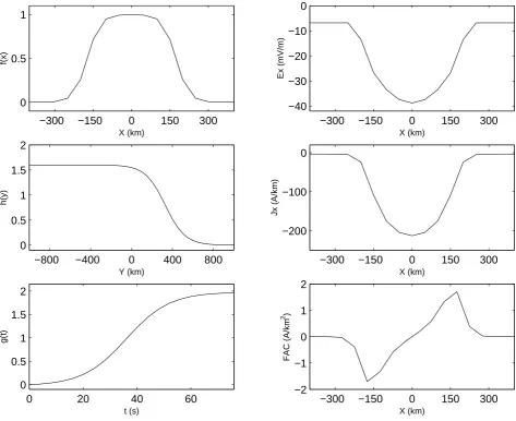
Our first example is an electrojet that intensifies and becomes more non-uniform with time. The input model is shown in Figs. 4 and 5. The electrojet flows in they-direction and the input electric fieldEpotis constant in time and uniform in they-direction. The cross section ofEpot_{over the electrojet}

is shown in the upper right panel of Fig. 4. The time varia-tions andy-dependence of the model are in the conductances, which are defined as

ΣP = ΣH/2, (3)

ΣH= 1 +f(x) [1 +h(y)g(t)]. (4)

Functionsf(x),h(y)andg(t)are given in the left side panels of Fig. 4. The calculation area where the CECS representing the induced electric field are placed is -625km≤x≤625

kmby -3025km≤y ≤3025km, with 50kmresolution in both directions. In the beginning the conductivity distribu-tions are uniform in they-direction. Cross sectional profiles of the resultingJ and FAC distributions are shown in mid-Fig. 1. Lenz’s law in the northern auroral ionosphere (with uniform conductances and downward pointing background magnetic field). Changes of the potential electric field (Epot) and associated currents (Jp and Jh) create rotational induced electric field (Eind). Induced currents oppose the change in rotational currents, but enhance the change in divergent currents (i.e. FAC).

– Calculate the magnetic fieldBcreated by the currents. – Faraday’s law relates the unknownEindto the magnetic

fieldB.

In the CECS representation Ohm’s law and Faraday’s law give us a system of linear algebraic equations that relate the unknown scaling factors of the CECS representation ofEind to the scaling factors of the input field Epot _and conduc-tances6H,6P. The CF and DF CECS have been defined so

that they have either a Diracδ-function curl or divergence at their center. This means that the calculation method is essen-tially a finite element method (FEM), where the basis func-tions (CECS) describe the curl and divergence of the elec-tric field. The CECS basis functions are very convinient for the ionospheric induction problem, for they make it easy to divide electric fields and currents into curl- and divergence-free parts, which is essential in the calculations. Moreover, use of the CECS basis converts spatial differential equations into systems of linear algebraic equations, where boundary conditions are implicitely included. Detailed description of the method is given in Vanham¨aki et al. (2006).

3 Features of ionospheric induction

3.1 Lenz’s law in the ionosphere

Lenz’s law states that the direction of the induced electric field in a loop of wire is such that the induced current op-poses the change of the magnetic flux through the loop. Fig-ure 1 is a schematic presentation of the ionospheric induction process. The potential electric field with associated Pedersen and Hall currents is on the left side. The potential E-field in-creases between T=1 and T=2 and the induced electric field and currents are on the right side. The inductive electric field is a rotational field, which (when conductances are uniform) is associated with a rotational Pedersen current and divergent

Hall current. The induced currents oppose the change in the rotational current, and hence also the change of magnetic flux through the ionospheric plane, but enhance the change in the divergent currents. This tendency of inductive currents to en-hance the change of FAC was also noted by Buchert (1998) and Yoshikawa and Itonaga (2000).

The z-component of the electric field is assumed to be very small due to very high conductivity along the magnetic field, so the rotationalEindis given by thez-component of Fara-day’s law,

(∇ ×Eind)z= − ∂Bz

∂t . (1)

In the CECS representation it is easy to see that only divergence-free currents are associated with the z-component of the magnetic field (Vanham¨aki et al., 2006, Eqs. 6–7). The induced electric field is also divergence-free, and according to Lenz’s law it opposes the change in the divergence-free currents. Therefore we can estimate

Eind≈ −µ0l ∂Jdf

∂t , (2)

wherel is a typical length scale andJdf _{is the ionospheric}

divergence-free current. These kind of estimates, when ap-plied to realistic data-dased models of different ionospheric current systems, are compared with exact results in Sect. 4. 3.2 Dependence on ionospheric parameters

0 10 20 30 40 50

Epot

mV/m

0 10 20 30 40 50

|Eind|

mV/m

−180 −90 0 90 180

arg(Eind)

deg

0 10 20

FAC1

A/km

2

0 20 40 60

|FACind|

A/km

2

−180 −90 0 90 180

arg(FACind)

deg

0 100 200

0 50 100

I1

ρ (km)

kA

0 100 200

0 100 200 300

|Iind|

ρ (km)

kA

0 100 200

−180 −90 0 90 180

arg(Iind)

ρ (km)

deg

Fig. 2. Input system (electric fieldEpot, field-aligned current density FAC1 and the total field-aligned current I1) is rotationally symmetric and oscillates harmonically in time. Upper row: Input electric field, and magnitude and phase of the induced electric fieldEind. Middle row: Same for the FAC. Bottom row: same for the integrated FAC inside radiusρ. In these examples conductances are uniform,6P=8 S and 6H=16 S. Oscillation timeT is varied:T=1,T=2,T=4,T=8andT=16.

the radiusρ=155 km is zero. This means that also the input current system is confined in this region. In the numerical calculations a rectangular 61×61 element grid with 10 km spacing was used. The situation with uniform conductances and harmonic time-dependence was discussed in Sect. 2.2 of Vanham¨aki et al. (2006). According to their Eq. (15) the in-duced electric field depends on the ratios6H/T and6P/T.

Here we vary each of the parametersT,6P and6H one at a

time, while keeping the other two fixed.

Figure 2 shows the input and induced electric field, FAC and integrated FAC for different oscillation times, between T=1 s andT=16 s. In this example ionospheric conductances are6P=8 S and6H=16 S. The top row of the figure shows

the radial profiles of the input potential electric field and the magnitude and phase (with respect to the input field’seiωt) of the induced rotational electric field for differentT. The middle and bottom rows show the FAC and its integral I (ρ)=2π

Z ρ

0

FAC(ρ0) dρ0,

0 10 20 30 40 50

Epot

mV/m

0 5 10 15 20

|Eind|

mV/m

−180 −90 0 90 180

arg(Eind)

deg

0 20 40 60 80

FAC1

A/km

2

0 10 20 30 40

|FACind|

A/km

2

−180 −90 0 90 180

arg(FACind)

deg

0 100 200

0 100 200 300

I1

ρ (km)

kA

0 100 200

0 100 200 300

|Iind|

ρ (km)

kA

0 100 200

−180 −90 0 90 180

arg(Iind)

ρ (km)

deg

Fig. 3. Similar to Fig. 2, but now the Pedersen conductance6P is varied while keeping the oscillation timeT and Hall conductance6H constant. In these examplesT=8 s and6H=30 S, while the Pedersen conductance is6P=30,6P=15,6P=10,6P=7.5and6P=6.

outside the area of changing currents. The induced electric field is also roughly 90 degrees behind the input field, at least near the origin, which is related to the fact thatEinddepends on the time derivative of the magnetic field.

The effect of different oscillation times on the induced fields is clearly visible in Fig. 2. With the shortest oscilla-tion time T=1 s the induced field Eind has a peak magni-tude similar to the input potential field, while withT=16 s the induced field is already quite small. When T >4 s the magnitude of the induced electric field depends almost lin-early on the frequencyω=2π/T. However, with smallerT the induced field increases less rapidly withω and is also more localized, decreasing faster at large distances. The FAC, shown in the middle row of Fig. 2, are concentrated near the origin and at the outer ring, where the sources of

−300 −150 0 150 300 0

0.5 1

X (km)

f(x)

−300 −150 0 150 300

−40 −30 −20 −10 0

X (km)

Ex (mV/m)

−800 −400 0 400 800

0 0.5 1 1.5 2

Y (km)

h(y)

−300 −150 0 150 300

−200 −100 0

X (km)

Jx (A/km)

0 20 40 60

0 0.5 1 1.5 2

t (s)

g(t)

−300 −150 0 150 300

−2 −1 0 1 2

X (km)

FAC (A/km

2 )

Fig. 4. On the left side the functionsf (x),h(y)andg(t )giving the spatial and temporal dependences of the electrojet model (Eq. 4). On the right side the cross sectional shape of the North-South directed electric field and current together with FAC.

than the input FAC, although Eind is at most equal to in-putEpot. This is partly explained by the larger spatial scale of the induced E-field and also by the ratio6H/6P=2 of

the conductances. In the input system rotational currents are Hall currents and FAC are associated with Pedersen cur-rents. In the induced system this is reversed, which means that max(FACind/FAC1)∝2 max(|Eind_|/|Epot_|).

Figure 3 shows the effect of varying Pedersen conductance 6P, while keeping the oscillation timeT and Hall

conduc-tance6H constant. The peak magnitude of the induced

elec-tric field increases slightly with decreasing6P, and the field

also decays somewhat slower with distance. This is related to the behaviour of the induced rotational currents, which are Pedersen currents in the case of uniform conductances. In-duction opposes the change in the z-component of the mag-netic field, which in turn depends on the rotational currents. Thus induced rotational currents, that get stronger with6P,

“screen” the input system, and make induced E-field slightly smaller and more localized. The induced FAC depend on

Hall conductivity and on the derivative of the induced elec-tric field in the radial direction. Therefore changing6P does

not affect induced FAC significantly, although the input FAC are varied linearly with6P.

In contrast to the non-trivial T and 6P dependences,

Eq. (15) of Vanham¨aki et al. (2006) shows that the induced electric field depends linearly on Hall conductance. This is reasonable, for induction depends on the temporal changes of the z-component of the magnetic field, as explained in the previous section. Bz on the other hand is associated with

rotational currents. In the case of uniform conductances, ro-tational currents of the input system are Hall currents, while rotational currents of the induced system are Pedersen cur-rents. Therefore increasing6H has the same effect on

in-duction as increasing the strength of the input electric field by some constant factor. ConsequentlyEinddepends linearly on 6H, and the induced FAC, which are Hall currents, depend

5

10

15

−300

−150

0

150

300

X (km)

Pedersen conductance, 1/Ω

10

20

30

−300

−150

0

150

300

Epot, max = 38.8 mV/m

X (km)

Eind, max = 4.3 mV/m

−300

−150

0

150

300

J1, max = 1323 A/km

X (km)

Jind, max = 147 A/km

−4

−2

0

2

4

−300

−150

0

150

300

X (km)

FAC1, A/km2

−0.5

0

0.5

0

10

20

−800 −400

0

400

800

−300

−150

0

150

300

Y (km)

X (km)

ratio Eind / Etot, max = 30 %

−50

0

50

−800 −400

0

400

800

Ratio FACind / FACtot, max =126 % , min =−274 %

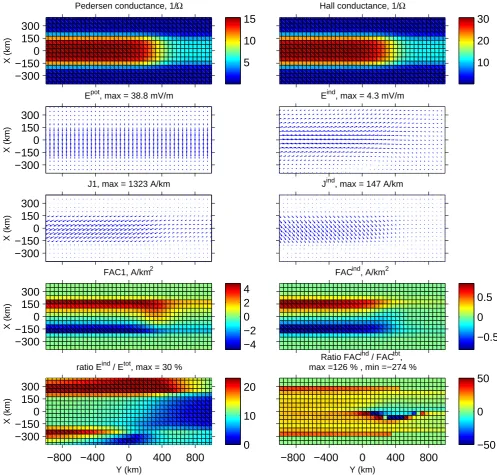
Fig. 5. The input electrojet model (Pedersen and Hall conductances, potential electric fieldEpotwith current systemJ1 and FAC1) and the calculated induced electric field (Eind) and current system (Jindand FACind) at time instantt=40 s. Comparison between the induced and total (input + induced) electric field and FAC are also shown.

4 Inductive fields in different ionospheric systems

Next we present results for three realistic ionospheric situ-ations, namely a non-uniform electrojet, WTS and-band. The electrojet model is based on models presented by Untiedt and Baumjohann (1993) and Amm (1995). The WTS and -band models have been published by Amm (1995) and Amm (1996). They are constructed from observational data ob-tained at northern Scandinavia by the Scandinavian

Magne-tometer Array, EISCAT radar and magneMagne-tometer cross, and STARE radar.

4.1 Non-uniform electrojet

−300 −150 0 150 300

J1p, max = 592 A/km

X (km)

Jpind, max = 66 A/km

−300 −150 0 150 300

J1h, max = 1183 A/km

X (km)

Jhind, max = 131 A/km

−300 −150 0 150 300

J1cf, max = 565 A/km

X (km)

Jcfind, max = 112 A/km

−800 −400 0 400 800 −300

−150 0 150 300

J1df, max = 1124 A/km

Y (km)

X (km)

−800 −400 0 400 800

Jdfind, max = 79 A/km

Y (km)

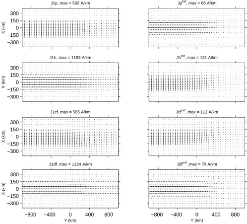
Fig. 6. The division of original (1) and induced (ind) currents of the electrojet model into Pedersen (Jp), Hall (Jh), curl-free (Jcf) and divergence-free (Jdf) parts at time instantt=40 s

the y-direction. The cross section ofEpotover the electrojet is shown in the upper right panel of Fig. 4. The time varia-tions and y-dependence of the model are in the conductances, which are defined as

6P =6H/2, (3)

6H =1+f (x)[1+h(y)g(t )]. (4)

Functions f (x), h(y) and g(t ) are given in the left side panels of Fig. 4. The calculation area where the CECS representing the induced electric field are placed is −625 km≤x≤625 km by −3025 km≤y≤3025 km, with

50 km resolution in both directions. In the beginning the con-ductivity distributions are uniform in they-direction. Cross sectional profiles of the resultingJx and FAC distributions

−300 −150 0 150 300

B1 at ground, max = 402 nT

X (km)

Bind at ground, max = 29 nT

−200 0 200

−300 −150 0 150 300

X (km)

B1z at ground

−20 −10 0 10

Bzind at ground

−300 −150 0 150 300

B1 at z=−300 km, max = 760 nT

X (km)

Bind at z=−300 km, max = 144.5 nT

−100 0 100

−800 −400 0 400 800

−300 −150 0 150 300

Y (km)

X (km)

B1z at z=−300 km

−10 −5 0 5

−800 −400 0 400 800

Y (km) Bzind at z=−300 km

Fig. 7. The magnetic fields associated with the input (B1) and induced (Bind) electrojet system at the ground and at 300 km above the ionospheric current layer at time instantt=40 s.

these kind of values have been observed during large storms (Pulkkinen et al., 2005).

The input and induced systems att=40 s are illustrated in Figs. 5–7. The input electrojet consists of a southward elec-tric field and South-West currents that are concentrated in the x-direction to a∼300 km wide channel, where also the conductances are enhanced. FAC are focused on two narrow bands at the northern and southern edges of the electrojet, ex-cept at the transition region where a downward FAC feed the intensifying ionospheric current. The induced electric field Eind is directed eastward and is quite uniform in the area where the input electrojet increases. In this area the induced E-field is about 10% of the input field. The induced E-field is not symmetric in the North-South direction, but spreads farther out in the North. This is clearly visible in the lower left panel of Fig. 5, where the ratio|Eind|/|Epot+Eind| is illustrated.

Table 1. Dependence of max(|Eind|) on the durationT of the electrojet intensification. In these examplesTis changed by a factor of 2 while keeping all other parameters fixed. Also the ratio between the maximum values ofEindfor differentT is given.

T 19 38 76 152 304 s

max(|Eind|) 12.31 7.74 4.30 2.24 1.14 mV

Ratio 1.59 1.80 1.92 1.96

5

10

15

20

−300

−150

0

150

300

X (km)

Pedersen conductance, 1/Ω

20

40

60

80

Hall conductance, 1/Ω

−300

−150

0

150

300

Epot, max = 31.04 mV/m

X (km)

Eind, max = 1.97 mV/m

−300

−150

0

150

300

J1, max = 742 A/km

X (km)

Jind, max = 145 A/km

−6

−4

−2

0

2

−300

−150

0

150

300

X (km)

FAC1, A/km2

−1

0

1

FACind, A/km2

0

10

20

30

−600 −300

0

300 600

−300

−150

0

150

300

Y (km)

X (km)

ratio Eind / Etot, max = 53 %

−100

0

100

−600 −300

0

300 600

Y (km)

Ratio FACind / FACtot,

max =244 % , min =−792 %

Fig. 8. Same as Fig. 5, but for the WTS model.

of upward FAC being∼80% of the downward FAC. This excess downward FAC feeds the intensifying western part of the electrojet. In the induced system there is∼15% im-balance in the opposite direction, whith the excess induced FAC flowing upwards in the transition region between the

−300

−150

0

150

300

J1p, max = 277 A/km

X (km)

Jpind, max = 37 A/km

−300

−150

0

150

300

J1h, max = 708 A/km

X (km)

Jhind, max = 140 A/km

−300

−150

0

150

300

J1cf, max = 323 A/km

X (km)

Jcfind, max = 98 A/km

−600 −300

0

300

600

−300

−150

0

150

300

J1df, max = 605 A/km

Y (km)

X (km)

−600 −300

0

300

600

Jdfind, max = 53 A/km

Y (km)

Fig. 9. Same as Fig. 6, but for the WTS model.

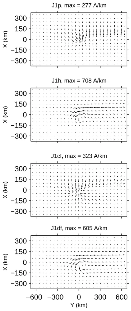
the input and induced current systems into Pedersen, Hall, curl-free and divergence-free parts is given in Fig. 6. The in-duced currents oppose the change of divergence-free currents but increase the change of curl-free currents and associated FAC. This behaviour is in accordance with Lenz’s law, as ex-plained in Sect. 3. Most of the FAC in the input model are associated with Pedersen currents, but in the induced system

−300 −150 0 150 300

Eind, max = 1.97 mV/m

X (km)

−600 −300 0 300 600

−300 −150 0 150 300

−d(J1df)/dt, max = 96 A/(s km)

Y (km)

X (km)

Fig. 10. Comparison between the induced electric field (same as in Fig. 8) and negative time derivative of the divergence-free currents of the input system.

are symmetric in the North-South direction, but the curl- and divergence-free currents are unsymmetric because of the ex-tra FAC flowing at the ex-transition region. The slight asym-metry of the divergence-free currents is the reason why the induced electric field is also asymmetric, as noted above.

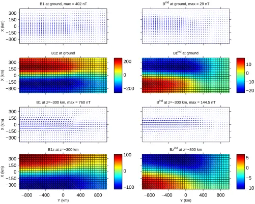
The magnetic fields associated with the input and induced current systems are illustrated in Fig. 7 at two different al-titudes, at ground and 300 km above the ionospheric current layer. At ground level the induced magnetic field opposes the change of the original field. The magnitude of the in-duced B-field is∼5% in the horizontal part and∼10% in the vertical part when compared to the original field. The asym-metry of the induced system is clearly visible, especially in the vertical component. Above the ionosphere the induced Bzis opposite to the original field, but the horizontal

compo-nent is rotated by almost 90 degrees. The magnitude of the inducedBzis again about 10%, but in the horizontal

compo-nent the magnitude of the induced field is over 15% of the original field. This larger contribution is mainly due to the induced FAC, that contribute to the horizontal magnetic field above the ionosphere.

In this example the intensification of the electrojet took place inT=76 s, as shown in the lower left panel of Fig. 4. In the numerical calculations this time interval was divided into 20 steps with1t=4 s. Table 1 shows the peak

magni-tudes of the induced electric field for different values ofT. In these examples only the total durationT of the electrojet intensification is changed while keeping the form of temporal variations and other parameters the same. ChangingT from 304 s to 152 s doubles the magnitude of the induced elec-tric field, as expected when all time derivatives are doubled. However, further decreases inT result in smaller increases in the induced field. The induction process becomes non-linear as the induced currents reach values that are comparable to the input system. When the intensification happens in time span of T=19 s the magnitude of the induced electric field is over 30% of the input potential field. This would mean that the maximum time derivative of the ground magnetic field is ∼51 nT/s, which is an exceptionally high, yet ob-served value (Pulkkinen et al., 2005). Interestingly, changes in the size (width) of the electrojet have exactly the same effect on the induced electric field as changes in the tempo-ral variations. It seems that the magnitude of the induced field depends (non-linearly) on the ratiol/τ, wherel andτ are characteristic spatial and temporal scales, respectively. A similar result was obtained by Yoshikawa and Itonaga (1996) for the case of Alfv´en wave reflection from ionosphere, while Buchert (1998) found dependencel2/τ.

4.2 WTS

The upper and left side panels of Fig. 8 show the input WTS model, Pedersen and Hall conductances 6P and 6H,

po-tential electric field Epotand associated currents and FAC. The calculation area where the CECS representing the in-duced electric field are placed is −625 km≤x≤625 km by −1025 km≤y≤1425 km, with 50 km resolution in both di-rections. Temporal variations are created by moving the whole system westward at 10 km/s, which is quite high but still a realistic speed (Paschmann et al., 2002, chapter 6). The maximum time derivative of the ground magnetic field in this case is∼5 nT/s. The induced electric fieldEindand currents Jindtogether with FAC are shown on the right side panels. The bottom panels of Fig. 8 show comparison of the induced E-field against the total field Epot_+Eind _{and induced FAC} agains the total FAC.

−300

−150

0

150

300

B1 at ground, max = 110 nT

X (km)

Bind at ground, max = 6.1 nT

−100

−50

0

−300

−150

0

150

300

X (km)

B1z at ground

−4

−2

0

2

4

Bzind at ground

−300

−150

0

150

300

B1 at z=−300 km, max = 409 nT

X (km)

Bind at z=−300 km, max = 114.6 nT

−40

−20

0

−600 −300

0

300

600

−300

−150

0

150

300

Y (km)

X (km)

B1z at z=−300 km

−1

−0.5

0

0.5

−600 −300

0

300

600

Y (km)

Bzind at z=−300 km

Fig. 11. Same as Fig. 7, but for the WTS model.

loop, with downward FAC at the eastern and upward FAC at the western part of the surge head. The induced FAC are al-most balanced with a slight upward net current, the integrated downward current over the analysis region being∼90% of the upward current in the same area. In the input model the imbalance is larger, the upward FAC being∼30% larger than the total downward FAC. It is interesting to note that while the induced upward FAC are concentrated at the same areas

where the FAC of the input system are largest, the induced downward FAC are located east of this area. This means that inductive processes do modify the nature of ionosphere-magnetosphere coupling, at least in the WTS.

0 10 20 30 40 50 60 70 80 0

1 2 3 4 5 6 7 8 9

V (km/s)

max |E

ind

| (mV/m)

Fig. 12. The peak magnitude of the induced electric field for dif-ferent velocities of the WTS system.

about the same magnitude (1.97 and 2.12 mV/m) and in both cases the induced field is concentrated in the same area at the surge head. However, the orientation and spatial structure of the induced field obtained by Vanham¨aki et al. (2005) is quite different from that found in this study. There are proba-bly two reasons for the differences: Vanham¨aki et al. (2005) calculated the induced field as a vacuum field (i.e. the sec-ond order effect of the induced current was ignored), and in their calculation method the induced field is not completely divergence-free.

Figure 9 shows the division of the input and induced cur-rents into different parts. In the previous electrojet example there was a high degree of similarity between the induced Pedersen and divergence-free currents and also between in-duced Hall and curl-free currents. In the WTS case the sim-ilarity is not as prominent, although the induced Hall and curl-free currents have very much the same shape if not mag-nitude. This is probably due to the larger and sharper con-ductivity gradient that are present near the surge head, where the induced electric field and currents are concentrated. In-deed, in the input system, which is spread out in a larger area, there is still a close connection between the Pedersen and curl-free currents as well as between Hall and divergence-free currents.

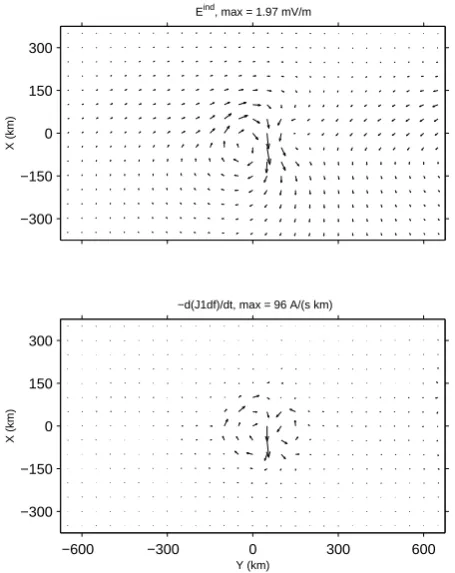
In the electrojet example it was easy to see that the induced electric field opposes the change in the divergence-free part of the input system. In the WTS example this is more difficult to see immediately from Fig. 9 due to the spatial movement of the system. Figure 10 shows a direct comparison between the induced electric field and the time derivative of the input divergence-free current. There is indeed a close resemblance between the two vector fields, in accordance to Lenz’s law as explained in Sect. 3. According to Fig. 10 typical length scale ofd(J1df)/dt seems to be about 100 km. Using this

length scale in Eq. (2) gives an estimate for the magnitude of the induced electric field as|Eind|≈12 mV/m, which is too high by a factor of 6.

Magnetic fields of the input and induced systems are shown in Fig. 11. The induced magnetic field at ground is almost negligible, less than 5% of the input field. Above the ionosphere, however, the horizontal part ofBindis quite large, about 30% of the input field near the surge head. Hor-izontal magnetic field above the ionosphere is dominated by FAC, which explains the large contribution of the induced field.

Figure 12 shows how the peak magnitude of the induced electric field varies with the speed of WTS, with other pa-rameters kept fixed. For all realistic speeds the dependence is linear. Only for speeds>30 km/s the induction process becomes non-linear, meaning that the induced currents them-selves produce a significant Bz, that affects induction via

Eq. (1). Also with these higher speeds the shape of the in-duced E-field is similar to Eind in Fig. 8, although the in-duced field spreads over a larger area.

4.3 -band

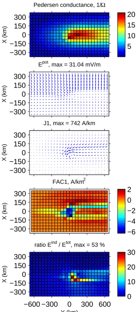
Our third example is an ionospheric -band. The in-put model and the induced electric field and current are given in Figs. 13–14. The calculation area where the CECS representing the induced electric field are placed is −625 km≤x≤675 km by −625 km≤y≤1075 km, with 50 km resolution in both directions. The input model is mov-ing eastward at 2 km/s, which is again in the upper range of realistic speeds in terrestrial applications. In this case the time derivative of the ground magnetic field is about 5 nT/s. In the case of the-band the induced electric fieldEind shown in Fig. 13 is very similar to that obtained by Van-ham¨aki et al. (2005) using a more approximate calculation method. The peak value of the induced field is very small compared to the largest values of the potential field present in the input model. However, the largest values ofEind oc-cur in theitself, i.e. in the area of enhanced conductivity, where the potential electric field is supressed. In this lim-ited area the inductive part contributes up to 25% of the total electric field.

5

10

15

20

−300

−150

0

150

300

X (km)

Pedersen conductance, 1/Ω

20

40

60

80

100

120

Hall conductance, 1/Ω

−300

−150

0

150

300

Epot, max = 188.91 mV/m

X (km)

Eind, max = 1.52 mV/m

−300

−150

0

150

300

J1, max = 2864 A/km

X (km)

Jind, max = 83 A/km

−20

−10

0

10

−300

−150

0

150

300

X (km)

FAC1, A/km2

0

1

2

FACind, A/km2

0

10

20

−150 100 350 600

−300

−150

0

150

300

Y (km)

X (km)

ratio Eind / Etot, max = 26 %

−50

0

50

100

−150 100 350 600

Y (km)

Ratio FACind / FACtot,

max =227 % , min =−79 %

Fig. 13. Same as Fig. 5, but for the-band model.

this means that also in this case ionospheric induction may change the ionosphere-magnetosphere coupling.

Figure 15 shows a comparison of the induced electric field with the time derivative of the divergence-free input system. Again, there is a good resemblance between the vector fields, although not as close as in the WTS case. Typical length

−300

−150

0

150

300

J1p, max = 939 A/km

X (km)

Jpind, max = 26 A/km

−300

−150

0

150

300

J1h, max = 2825 A/km

X (km)

Jhind, max = 79 A/km

−300

−150

0

150

300

J1cf, max = 894 A/km

X (km)

Jcfind, max = 62 A/km

−150 100 350 600

−300

−150

0

150

300

J1df, max = 2159 A/km

Y (km)

X (km)

−150 100 350 600

Jdfind, max = 31 A/km

Y (km)

Fig. 14. Same as Fig. 6, but for the-band model.

of the divergence-free input currents. The exact calculation gives a somewhat smoother vector field, which also spreads out in a larger area than whered(J1df )/dtis concentrated. This kind of smoothing is expected, since the real induc-tion process is non-local both in space and in time. Fur-thermore, estimates in Figs. 10 and 15 were calculated using

The magnetic field associated with the induced currents of the-band is shown in Fig. 16. The induced B-field is in practise negligible in comparison with the original magnetic field. Only the induced horizontalBind_⊥ above the ionosphere reaches values∼6% of the input field. This reflects the fact that in the-band the induced horizontal currents are rela-tively small when compared to the currents in the input sys-tem, but the induced FAC have a somewhat larger impact. The relatively wide and smooth distribution of the input FAC also means that the associated B-field above the ionosphere is quite featureless. The induced B-field is more concentrated, so it is able to modify the magnetic signature of the-band above the ionosphere to some extent.

5 Summary and conclusions

We have calculated the induced electric fields and current that are present in some typical ionospheric systems. The calculation was performed using the method presented by Vanham¨aki et al. (2006). In this calculation method the iono-spheric potential electric fieldEpotand height integrated con-ductances6P and6H are given as input. Output is the

in-duced rotational electric fieldEind in the ionosphere. The main difference to previous methods, e.g. Yoshikawa and Itonaga (1996), Buchert (1998) and Lysak (2004), is that we do not have to specify the Alfv´en waves incident from the magnetosphere, but can use more easily measurable iono-spheric parameters as input. The calculation method of Van-ham¨aki et al. (2006) can be used with general, non-uniform and time-dependent conductance distributions, which en-ables us to use very realistic data-based ionospheric models, as is done in Sect. 4.

The simplified examples presented in Sect. 3 clarify the effect of ionospheric conductances and characteristic time scales on the induction process. In these examples, for the sake of clarity we assume uniform conductances, unlike in the realistic examples presented in Sect. 4. We find that the induced electric field depends on the ratios6H/T and 6P/T. Increasing the Hall conductance increases the

in-duced electric field linearly and the inin-duced FAC as62_H. The effect of a varying Pedersen conductance is smaller. With large6P the induced electric field is somewhat decreased in

magnitude and becomes concentrated in a smaller area. The effect of varying oscillation timeT is a combination of the effects of varying6P and6H.

We also considered three typical examples of ionospheric electrodynamic situations, namely an intensifying electrojet, a westward travelling surge and an-band. All these models are realistic and based on observational data. In the WTS and -band models the induced electric field is concentrated in a rather small area, where the temporal changes of the cur-rent system are largest. The induced fieldEindis quite sig-nificant in these “hot-spots”, reaching values 20–50% of the potential field. Because the hot-spots are located in areas of

−300 −150 0 150 300

Eind, max = 1.52 mV/m

X (km)

−150 100 350 600

−300 −150 0 150 300

−d(J1df)/dt, max = 57 A/(s km)

Y (km)

X (km)

Fig. 15. Same as Fig. 10, but for the-band model.

enhanced conductances, even relatively small electric fields are associated with large ionospheric currents and FAC. In these two examples the induced currents form small local-ized loops, which modify the pattern of the otherwise present non-inductive currents. In the example of the non-uniform, intensifying electrojet the induced electric field has a mag-nitude of∼10% of the potential E-field in large parts of the system. Also the induced FAC are spread in a large area and contribute about 20% of the total FAC in the electro-jet. The induced currents are also associated with magnetic fields, that may have a significant contribution to the total B-field, especially above the ionospheric current sheet.

−300

−150

0

150

300

B1 at ground, max = 414 nT

X (km)

Bind at ground, max = 5.1 nT

−400

−200

0

200

−300

−150

0

150

300

X (km)

B1z at ground

−8

−6

−4

−2

0

2

Bzind at ground

−300

−150

0

150

300

B1 at z=−300 km, max = 1204 nT

X (km)

Bind at z=−300 km, max = 77.4 nT

−150

−100

−50

0

50

−150 100 350 600

−300

−150

0

150

300

Y (km)

X (km)

B1z at z=−300 km

−2

−1

0

−150 100 350 600

Y (km)

Bzind at z=−300 km

Fig. 16. Same as Fig. 7, but for the-band model.

Eq. (2) the magnitude of the induced field was over-estimated by a factor of 5–10 in all three cases, although the rather ar-bitrary determination of a characteristic length scale may be part of the reason. Futhermore, the ionospheric divergence-free currents are almost the same as the ionospheric equiv-alent currents that may be estimated using ground based

Our results, although limited to three specific events, show that locally inductive phenomena have an important role in (terrestrial) ionospheric electrodynamics. Induced electric fields in the ionosphere change the structure of the pure po-tential field that is mapped from the magnetosphere along field lines, and also induced FAC alter the coupling between the ionosphere and magnetosphere. Inductive effects are largest in the most dynamical events, which are usually the most interesting ones.

The calculation method presented by Vanham¨aki et al. (2006) that is used in this study assumes a 2-dimensional thin-sheet ionosphere. While this is a widely used and usually good enough approximation, the real 3-dimensional structure of the ionospheric currents may affect the induction process. A first step towards a 3-dimensional induction could be made by generalizing the calculation method presented by Vanham¨aki et al. (2006) to incorporate two ionospheric cur-rent sheets at diffecur-rent altitudes. The upper and lower sheets would contain mainly Pedersen and Hall currents, respec-tively. Already this simplistic 2-layer model would contain new features, like mutual induction and current closure be-tween the two sheets.

Another interesting future study would be to obtain obser-vational data on the ionospheric induction process. One pos-sibility would be to observe Alfv´en waves at the magneto-sphere both before and after they reflect from the ionomagneto-sphere using the Cluster spacecraft. Simultaneous observations of the ionospheric reflection area by a network of groundbased radars and magnetometers would allow us to compare the measured properties of the reflected waves with theoretical models.

Acknowledgements. The work of H. Vanham¨aki is supported by the Finnish Graduate School in Astronomy and Space Physics.

Topical Editor M. Pinnock thanks J. Vogt and another referee for their help in evaluating this paper.

References

Amm, O.: Direct determination of the local ionospheric Hall con-ductance distribution from two-dimensional electric and mag-netic field data: Application of the method using models of typi-cal ionospheric electrodynamic situations, J. Geophys. Res., 100, 21 473–21 488, 1995.

Amm, O.: Improved electrodynamic modeling of an omega band and analysis of its current system, J. Geophys. Res., 101, 2677– 2683, 1996.

Amm, O.: Ionospheric elementary current systems in spherical co-ordinates and their application, J. Geomagnetism and Geoelec-tricity, 49, 947–955, 1997.

Buchert, S.: Magneto-optical Kerr effect for a dissipative plasma, J. Plasma Phys., 59, 39–55, 1998.

Buchert, S. and Budnik, F.: Field-aligned current distributions gen-erated by a divergent Hall current, Geophys. Res. Lett., 24, 297– 300, 1997.

Janhunen, P.: On the possibility of using an electromagnetic iono-sphere in global MHD simulations, Ann. Geophys., 16, 397–402, 1998,

http://www.ann-geophys.net/16/397/1998/.

Kamide, Y., Richmond, A., and Matsushita, S.: Estimation of iono-spheric electric fields, ionoiono-spheric currents, and field-aligned currents from ground magnetic records, J. Geophys. Res., 86, 801–813, 1981.

Lysak, R.: Magnetosphere-ionosphere coupling by Alfv´en waves at midlatitudes, J. Geophys. Res., 109, A07201, doi:10.1029/2004JA010454, 2004.

Lysak, R. and Song, Y.: A three-dimensional model of the prop-agation of Alfv´en waves through the auroral ionosphere: First results, Adv. Space Res., 28, 813–822, 2001.

L¨uhr, H., Aylward, A., Buchert, S., Pajunp¨a¨a, K., Holmboe, T., and Zalewski, S.: Westward moving dynamic substorm features observed with the IMAGE magnetometer network and other ground-based instruments, Ann. Geophys., 16, 425–440, 1998, http://www.ann-geophys.net/16/425/1998/.

Paschmann, G., Haaland, S., and Treumann, R. (Eds.): Auroral Plasma Physics, Space Sci. Rev., 103, 1–486, 2002.

Pulkkinen, A., Lindahl, S., Viljanen, A., and Pirjola, R.: Geomag-netic storm of 29–31 October 2003: GeomagGeomag-netically induced currents and their relation to problems in the Swedish high-voltage power transmission system, Space Weather, 3, S08C03, doi:10.1029/2004SW000123, 2005.

Richmond, A. and Kamide, Y.: Mapping electrodynamic features of the high-latitude ionosphere from localized observations: Tech-nique, J. Geophys. Res., 93, 5741–5759, 1988.

Ruohoniemi, J. and Baker, K.: Large-scale imagining of high-latitude convection with Super Dual Auroral Radar Network HF radar observations, J. Geophys. Res., 103, 20 797–20 811, 1998. Sciffer, M., Waters, C., and Menk, F.: Propagation of ULF waves through the ionosphere: Inductive effect for oblique magnetic fields, Ann. Geophys., 22, 1155–1169, 2004,

http://www.ann-geophys.net/22/1155/2004/.

Untiedt, J. and Baumjohann, W.: Studies of polar current systems using the IMS Scandinavian magnetometer array, Space Sci. Rev., 63, 245–390, 1993.

Vanham¨aki, H., Viljanen, A., and Amm, O.: Induction Effects on Ionospheric Electric and Magnetic Fields, Ann. Geophys., 23, 1735–1746, 2005,

http://www.ann-geophys.net/23/1735/2005/.

Vanham¨aki, H., Amm, O., and Viljanen, A.: New Method for Solv-ing Inductive Electric Fields in the Non-Uniformly ConductSolv-ing Ionosphere, Ann. Geophys., 24, 2573–2582, 2006,

http://www.ann-geophys.net/24/2573/2006/.

Yoshikawa, A. and Itonaga, M.: Reflection of shear Alfv´en waves at the ionosphere and the divergent Hall current, Geophys. Res. Lett., 23, 101–104, 1996.