www.ann-geophys.net/25/1279/2007/ © European Geosciences Union 2007
Annales
Geophysicae
Polar vortex evolution during Northern Hemispheric winter 2004/05
T. Chshyolkova1, A. H. Manson1, C. E. Meek1, T. Aso2, S. K. Avery3, C. M. Hall4, W. Hocking5, K. Igarashi6, C. Jacobi7, N. Makarov8, N. Mitchell9, Y. Murayama6, W. Singer10, D. Thorsen11, and M. Tsutsumi2
1Institute of Space and Atmospheric Studies, University of Saskatchewan, 116 Science Place, Saskatoon, SK, S7N 5E2,
Canada
2National Institute of Polar Research, Tokyo, Japan 3CIRES, University of Colorado, Boulder, USA
4Tromsø Geophysical Observatory, University of Tromsø, Tromsø, Norway
5Department of Physics and Astronomy, University of Western Ontario, London, Canada 6National Institute of Information and Communications Technology, Tokyo, Japan 7Institute for Meteorology, University of Leipzig, Leipzig, Germany
8Institute for Experimental Meteorology, SPA “Typhoon”, Obninsk, Russia
9Centre for Space, Atmospheric, and Oceanic Sciences, Department of Electronic and Electrical Engineering, University of
Bath, Bath, UK
10Leibniz-Institut fur Atmospharen physik an der Universitat Rostock, K¨uhlungsborn, Germany 11Department of Electrical and Computer Engineering, University of Alaska, Fairbanks, USA
Received: 20 February 2007 – Revised: 28 May 2007 – Accepted: 12 June 2007 – Published: 29 June 2007
Abstract. As a part of the project “Atmospheric Wave Influences upon the Winter Polar Vortices (0–100 km)” of the CAWSES program, data from meteor and Medium Fre-quency radars at 12 locations and MetO (UK Meteorologi-cal Office) global assimilated fields have been analyzed for the first campaign during the Northern Hemispheric winter of 2004/05. The stratospheric state has been described using the conventional zonal mean parameters as well as Q-diagnostic, which allows consideration of the longitudinal variability.
The stratosphere was cold during winter of 2004/05, and the polar vortex was relatively strong during most of the win-ter with relatively weak disturbances occurring at the end of December and the end of January. For this winter the strongest deformation with the splitting of the polar vortex in the lower stratosphere was observed at the end of Febru-ary. Here the results show strong latitudinal and longitudinal differences that are evident in the stratospheric and meso-spheric data sets at different stations. Eastward winds are weaker and oscillations with planetary wave periods have smaller amplitudes at more poleward stations. Accordingly, the occurrence, time and magnitude of the observed reversal of the zonal mesospheric winds associated with stratospheric disturbances depend on the local stratospheric conditions. In general, compared to previous years, the winter of 2004/05 could be characterized by weak planetary wave activity at stratospheric and mesospheric heights.
Correspondence to: T. Chshyolkova ([email protected])
Keywords. Meteorology and atmospheric dynamics (Mid-dle atmosphere dynamics; Waves and tides) – Radio science (Remote sensing)
1 Introduction
The stratospheric polar vortex, a system of strong eastward winds, is the main dynamical feature of the winter middle atmosphere (20–100 km) at middle and high latitudes. Each day after the autumnal equinox less sunlight reaches the po-lar stratosphere, and as a consequence, the primary heating due to ozone decreases. As a result of the radiational cool-ing at high latitudes a strong negative temperature gradient develops between polar and tropical regions. This leads to the formation of the polar night jet, comprising strong east-ward winds encircling the pole. These winds reach speeds of∼80 m/s at∼60 km altitude in the Northern Hemisphere (NH) and isolate polar air (the core of the polar vortex) from air in the tropics and middle latitudes (Schoeberl and Hart-mann, 1991; Wallace and Hobbs, 2006). Therefore the polar vortex not only dominates the dynamics, it also has a pro-found effect on the distribution of chemical constituents.
downward motion at higher latitudes is responsible for a much warmer mesopause and even stratopause than would be expected from considerations of radiative equilibrium.
The NH polar vortex is highly variable throughout its life cycle. Intervals of a strong vortex (symmetrical and cen-tered over the pole) with high wind speeds are interrupted by sudden stratospheric warmings (SSW). During SSW strato-spheric temperatures significantly increase (at least 25 K per week) at higher latitudes (>50◦). The stratospheric warm-ing is called major (MSW) if the temperature enhancement leads to reversal of the middle latitude-to-pole temperature-gradient and results in reversal of the mean zonal winds from eastward to westward at heights near 30 km. Usually a MSW develops in the middle of winter, after the solstice. If there is no reversal of the mean zonal circulation then the strato-spheric warming is called minor. The warming that occurs in late winter/early spring, and marks the transition from win-ter to summer circulation, is the final warming. There is also one more type of warming, the so-called Canadian warm-ing, which occurs as a result of intensification of the Aleu-tian anticyclone with a reversal of the temperature gradient poleward of 60◦N over Canada.
Labitzke (1972) investigated temperature changes in the middle atmosphere at higher latitudes (circa 65◦N), during stratospheric warmings, using satellite radiance and rocket measurements. The results indicated that the effects of strato-spheric mid-winter warmings extend into the upper meso-sphere. It was shown that at first the temperature increases around 60 km height. Then over several days the middle stratosphere warms up, while the lower stratosphere and up-per mesosphere cool. During the breakdown of the vortex, temperatures rise in the lower stratosphere and upper meso-sphere and decrease in the layer between 30 and 60 km.
At mesospheric heights reversals of the dominating east-ward winds have been observed in association with strato-spheric disturbances (Gregory and Manson, 1975; Greisiger et al., 1984; Jacobi et al., 1997; Hoffmann et al., 2002). Hoff-mann et al. (2002) studied the response of the mesospheric winds, which were measured with Medium Frequency (MF) radars, to stratospheric circulation disturbances at Juliusruh (55◦N) during 1989–2000 and at Andenes (69◦N) during 1998–2000. Reversals of mesospheric winds were observed on days near those of stratospheric warmings and of en-hanced activity of quasi-stationary waves. However, clear coincidences between stratospheric and mesospheric events occurred only for planetary-scale phenomena. It was also noted that wind reversals occurred at different times at the two stations, with the later reversal at the more poleward sta-tion (Andenes). Some cases, when the mesospheric zonal winds decreased and/or reversed during cold stratospheric condition, were reported as well (Greisiger et al., 1984).
Another European study (Jacobi et al., 2003) involved mesospheric radar wind measurements over Castle Eaton (52◦N), Collm (52◦N) and Esrange (68◦N) during the February 2001 major stratospheric warming. They also
found that the warming resulted in a reversal of both the zonal and meridional wind components. Earlier, Jacobi et al. (1997) had argued that although the beginning of the warming at low stratospheric heights (∼20 km) often appears simultaneously with the weakening or reversal of the meso-spheric zonal winds (∼90 km), this is not the result of large vertical scale or wavelength process, but is rather due to the fact that the warming needs approximately the same time to reach the lower stratosphere and the mesosphere from the stratopause, where it starts. Both Hoffmann et al. (2002) and Jacobi et al. (2003) observed long period oscillations around 10 and 20 days in their radar data. The 20-day spec-tral peak was assumed to be merely the response time of the MLT winds to the stratospheric warming, while the 10-day spectral peak could have been the signature of a planetary wave propagating from below. Therefore the variability at the mesospheric heights could be the result of the combined effect of a vertically propagating planetary wave and decreas-ing zonal winds, i.e. a trend rather than an oscillation. Man-son et al. (2002) using both radar winds and airglow inten-sities during the SSW and final warmings of several winters, found no relationship between these events and phases of the long period oscillations associated with planetary waves.
During the same stratospheric warming event (February 2001) that had been studied by Jacobi et al. (2003), hydroxyl (∼86 km) and oxygen green line (∼97 km) emissions were measured using a ground-based wide angle Michelson Inter-ferometer at Resolute Bay, Canada (75◦N, 95◦W). Winds obtained by Doppler-shifting techniques from both emission layers showed reversals around the times of SSW (Bhat-tacharya et al., 2004). Spectral analyses of the data indicated that during the periods of cold or undisturbed stratospheric temperatures the amplitudes of oscillations with periods from 6 h to 2 days decreased. The authors also noted an increase in short (<12 h) period oscillations over the course of the warming.
downward. The region of warm temperatures at high lati-tudes starts to descend.
The model (Matsuno, 1971) predicts a decrease in tem-perature above the critical level at high latitudes, which is much smaller than the increase beneath it. Holton (1983) ar-gued that cooling due only to adiabatic ascent near the critical level is not enough to explain the observed decrease of meso-spheric temperatures during the SSW, especially when the critical level descends to the lower heights. Using a numer-ical model with a simple GW spectrum the author demon-strated that a significant temperature decrease in the meso-sphere resulted. This was caused by a reduction of the mean poleward meridional circulation due to a decrease of the GW drag followed by a relaxation toward radiative equilibrium. The decrease of GW drag was considered to be a result of the changed propagation conditions for GW in the lower at-mosphere during the course of a SSW event.
More recently Liu and Roble (2002) carried out a nu-merical study of the impact of a self-generated stratospheric warming on the Mesosphere/Lower Thermosphere (MLT) region. The Thermosphere, Ionosphere, Mesosphere, and Electrodynamics General Circulation Model/Climate Com-munity Model (TIME-GCM/CCM3), which is a new gen-eration GCM with GW parameterization, was used. They showed that growth of the planetary wave with the zonal wave number m=1 precedes the SSW, and that this growth could be due to wave resonance. The resonant amplifica-tion of the wave causes the deceleraamplifica-tion and reversal of the zonal wind and induces poleward and downward (the latter at high latitudes) circulation in the stratosphere and equa-torward circulation in the lower mesosphere. These lead to the adiabatic warming in the polar stratosphere (<25 K) and strong cooling (∼40 K) in the lower mesosphere. The au-thors (Liu and Roble, 2002) also demonstrated that changes in the wind field alter the propagation conditions for gravity waves (GW), so that more eastward GW can reach the MLT region during the warming, where they can cause weaken-ing and eventual reversal of the newly formed westward jet. The resulting vertical gradient of the winds is consistent with a cool polar mesosphere. The dissipation of GW at meso-spheric heights may also generate planetary waves in situ (Smith, 1996).
The CAWSES program (Climate and Weather of the Sun Earth System; SCOSTEP 2004-08) has offered more collab-orative opportunities to study the winter polar vortices, in particular the strong longitudinal differences that are evident in wind measurements from different stations, i.e. the occur-rence, time and magnitude of the reversals of the zonal meso-spheric winds (Smith et al., 1982). For the project “Atmo-spheric Wave Influences upon the Winter Polar Vortices (0– 100 km)”, wind data from several radars at 12 mid- and high-latitude locations and global assimilated fields from a GCM have been analyzed for the first campaign during the North-ern Hemispheric winter of 2004/05. Data and their analyses are described in Sects. 2 and 3, respectively. The evolution
of the stratospheric vortex over the Arctic during the win-ter is presented in Sect. 4, while Sect. 5 deals with the issue of stratosphere-mesosphere coupling. Section 6 provides a summary.
2 Data
2.1 Radar data
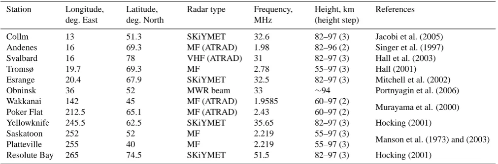
To study dynamics at the mesospheric heights (60–100 km) the meridional (NS) and zonal (EW) components of the winds obtained by Medium (MF) and Very High Frequency (VHF) radars are used. The daily mean wind data from se-lected heights were provided by 12 mid- and high-latitude stations. The coordinates of the stations, main parameters and references that contain more detailed description of these radars are given in Table 1.
All MF radars are of similar configuration; they employ the spaced antenna technique to detect motions of weakly ionized irregularities in the ionospheric D and lower E re-gions. To estimate wind velocities from the raw data, two different methods, the spaced antenna “full correlation anal-ysis” by Meek (1980) and a more classical analysis by Briggs (1984), were used. Thayaparan et al. (1995) compared winds calculated using these two methods and found no significant difference between them.
Meteor radars detect the part of transmitted energy that is scattered back by the meteor’s trail of ionized gas. Then the atmospheric wind velocities are deduced by observing how the meteor trail drifts with time (Doppler shifting). All of the meteor radars (except Obninsk) are commercially produced HF/VHF All-Sky Interferometric Meteor Radars by ATRAD (Atmospheric Radar Systems Pty Ltd, Australia) or MAR-DOC (Modular Antenna Radar Designs Of Canada) together with Genesis Software Pty, Ltd (SKiYMET). These VHF all-sky systems employ interferometric techniques and operate at very high pulse repetition frequencies (∼2 kHz). Such frequencies allow the determination of additional meteor pa-rameters such as entrance speeds. Description of the hard-ware, detection algorithms and data handling can be found in the paper by Hocking et al. (2001).
Both meteor and MF radars provide horizontal winds in the MLT region. However, they employ different measure-ment techniques, use different assumptions for the wind es-timation, and have their own limitations. For example, the fields of view are approximately ±17◦ and ±70◦ for MF
Table 1. Characteristics of the radars.
Station Longitude,
deg. East
Latitude, deg. North
Radar type Frequency,
MHz
Height, km (height step)
References
Collm 13 51.3 SKiYMET 32.6 82–97 (3) Jacobi et al. (2005)
Andenes 16 69.3 MF (ATRAD) 1.98 82–96 (2) Singer et al. (1997)
Svalbard 16 78 VHF (ATRAD) 31 82–97 (3) Hall et al. (2003)
Tromsø 19.7 69.3 MF 2.78 55–97 (3) Hall (2001)
Esrange 20.4 67.9 SKiYMET 32.5 82–97 (3) Mitchell et al. (2002)
Obninsk 36 52 MWR beam 33 ∼94 Portnyagin et al. (2006)
Wakkanai 142 45 MF (ATRAD) 1.9585 60–97 (2)
Murayama et al. (2000)
Poker Flat 212.5 65.1 MF (ATRAD) 2.43 60–97 (2)
Yellowknife 245.5 62.5 SKiYMET 35.65 82–97 (3) Hocking (2001)
Saskatoon 252 52 MF 2.219 55–97 (3)
Manson et al. (1973) and (2003)
Platteville 255 40 MF 2.219 55–97 (3)
Resolute Bay 265 74.5 SKiYMET 51.5 82–97 (3) Hocking (2001)
locations (Australia, Canada, and Norway), the conclusions are similar. The mesospheric wind velocities as determined by meteor and MF radars demonstrate good agreement below 90 km. In general the MF meridional wind speeds are sys-tematically lower by 20%, while the zonal component shows “modestly altitude-dependent” differences (Hall et al., 2005). It is necessary to keep this in mind when measurements from radars are considered below (Sect. 5).
2.2 MetO data
MetO (also known as UKMO, United Kingdom Meteorolog-ical Office) temperatures and horizontal wind components have been used to describe the state of the stratosphere. The MetO data are the result of assimilation of operational meteo-rological measurements from satellites, radiosondes, and air-craft into a numerical forecasting model of the stratosphere and troposphere. Since November 2000 the MetO fields have been produced using a 3-D variational (3DVAR) data assim-ilation system (Lorenc et al., 2000). After October 2003 the “New Dynamics” version of the “Unified Model” was intro-duced and three more levels (up to 0.1 hPa≈64 km) added to the existing 22 standard UARS (Upper Atmosphere Research Satellite) pressure levels. The outputs of the model with data assimilation are global fields of daily temperatures, geopo-tential heights and wind components. There are 72 latitudes and 96 longitudes with 2.5◦ and 3.75◦ steps in latitude and
longitude, respectively.
Estimates of the errors in the analysed fields are 1◦K and 6 m/s at low heights (<100 hPa). These estimations are from the documentation provided by the team of the Met Of-fice through the British Atmospheric Data Centre (BADC, http://badc.nerc.ac.uk/). In general, the errors are predicted to be larger at high latitudes and at the uppermost levels. In-tercomparisons of different climatological data sets for the
middle atmosphere (UKMO, ECMWF, NCEP, CIRA86, etc.) reveal uncertainties and problem areas (Randel et al., 2004). The MetO data, for instance, show cold temperature-biases (∼5 K) near the stratopause (the upper levels of the model) and a warm tropical tropopause temperature (∼1–2 K). Note, however, that the data used for these comparisons were from earlier years (1992–1997), before later improvements in the model and assimilation technique. MetO data are widely used and shown to be very helpful in studies of the strato-spheric region. In particular, O’Neill et al. (1994) success-fully used the MetO data to study the evolution of the NH stratosphere during winter 1991/92. We have also used MetO data in conjunction with TOMS (Total Ozone Mapping Spec-trometer) and MF radar data in earlier studies (Chshyolkova et al., 2005).
2.3 Aura data
As a supplement we have also employed temperatures mea-sured by the Microwave Limb Sounder (MLS, Waters et al., 2006) on board the National Aeronautic and Space Admin-istration (NASA) Aura satellite. The Aura spacecraft was launched on 15 July 2004 on a 705-km sun-synchronous near-polar orbit with a 98.2 inclination. It has a 16-day “re-peat cycle” and 233 revolutions per cycle. The temperatures used here are MLS data produced by the “version 1.5” data processing algorithms (along the measurement track). The daily data are available for the 316–0.001 hPa (∼8–80 km) altitude region and have coverage from 82◦S to 82◦N lati-tudes on each orbit with horizontal and vertical resolutions of 500 km and 4 km, correspondently. The first validation results of Froidevaux et al. (2006) show that MLS measure-ments of temperature and mixing ratios of O3, H2O, N2O,
HCl, HNO3, and CO agree well with other satellite and
in the stratospheric and mesospheric regions. The precision of a single temperature profile was estimated to be 0.5–1 K in the middle stratosphere and noisier (estimated precision up to 2 K) at the lowest (316 hPa) and highest (0.001 hPa) pres-sure levels. The special issue on Aura (IEEE Transactions on Geoscience and Remote Sensing 44(5), May 2006) offers more detailed information on the technical characteristics of the instrument and retrieval algorithms.
3 Analysis
To characterize the winter polar vortex the “Q-diagnostic” has been chosen and the algorithm developed by Harvey et al. (2002) was closely followed. The Q-diagnostic includes calculation of the scalar quantity Q, the streamfunction (ψ ), the relative vorticity (ζ ), and integration of Q,ζ, and winds alongψ isopleths. Q is “a measure of the relative contribu-tion of strain and rotacontribu-tion in the wind field” (Fairlie, 1995), and for two-dimensional flow it is given by
Q= 1
2a2 (
1
cosϕ ∂u
∂λ−vtanϕ
2 +
∂v
∂ϕ
2
+2∂u
∂ϕ
1
cosϕ ∂v
∂λ+utanϕ
, (1)
whereφ is latitude, λ is longitude, u is zonal wind, v is meridional wind, anda is the radius of the Earth. In areas whereQis positive the strain dominates and fluid elements are stretched, and in regions with negativeQrotation dom-inates the flow. For example, shear-zones beyond the edges of vortices and near jet streams have positiveQwhile neg-ativeQis associated with stable rotational flow (Babiano et al., 1994) and is generally observed inside vortices. How-ever, as was noted by Harvey et al. (2002), in the presence of elongated vortices (cyclonic and anticyclonic) and polar vortex divisions shear-zones can also be found inside vor-tices. Therefore, for identification of the vortex edges the integrated values ofQalong streamfunction lines are used. Those streamlines that haveHQ≈0 and the strongest inte-grated winds are chosen to represent the vortex “edges”. The integration of relative vorticity along the streamlines enables one to distinguish cyclonic and anticyclonic vortices. A more detailed description of the Q-diagnostic can be found in Fair-lie (1995) and Harvey et al. (2002), and references therein.
4 Evolution of the polar vortex during winter of 2004/05
The NH winter of 2004/05 was relatively cold, especially in the lower stratosphere. More days and larger areas with tem-peratures below 195 K were observed during this Arctic win-ter (Manney et al., 2006). Due to decreases in temperature, a reduction of up to∼0.5 ppmv in water vapor was detected over Spitsbergen in the∼12–20 km height region on 25–27 January due to ice formation (Jim´enez et al., 2006). Figure 1
MetO: Zonal mean temperature at 10.0 hPa
300 350 400 450
day # of 2004/05 200
210 220 230
Temperature,K
MetO: Zonal mean NS wind component at 10.0 hPa
300 350 400 450
day # of 2004/05 -3
-2 -1 0 1 2 3
NS wind, m/s
Zonal mean EW wind component at 10.0 hPa
300 350 400 450
day # of 2004/05 -20
0 20 40 60 80
[image:5.595.310.547.60.417.2]EW wind, m/s
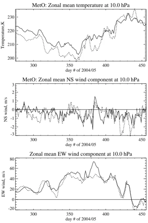
Fig. 1. Temperature (top), NS (middle) and EW (bottom) wind
components from MetO 10 hPa level averaged along the 60◦N
(solid) and 70◦N (dashed) longitudinal circles for the time interval
from 1 October 2004 till 31 March 2005 (day numbers 275–456).
shows variations of MetO temperatures (top panel), merid-ional (NS, middle panel) and zonal (EW, bottom panel) wind components averaged around the 60◦N (solid line) and 70◦N (dotted line) latitudinal circles at the 10 hPa pressure level (∼32 km), for the time interval from October 2004 (start-ing from day number 275) until the end of March 2005 (day number 456). The MetO temperatures (top) decrease until the end of December (day number 366) down to 202 K and 180 K at 60◦N and 70◦N, respectively, and exhibit similar
temporal variations at both latitudes, with temperatures aver-aged over 70◦N being lower than those averaged over 60◦N.
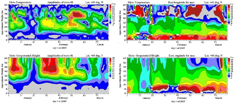
Fig. 2. Time (January–March) versus height (∼0–64 km) contours of the amplitudes (left) and phases (right) of the wave number 1 tem-perature (top) and geopotential height (bottom) perturbations. The phase is defined as longitude (east of Greenwich meridian) of the wave maximum.
more eastward) as winter proceeds with the strongest winds (up to 70 and 55 m/s at 60◦N and 70◦N, respectively) in
De-cember and January. After that, zonal winds decrease and become westward in the second part of March; this is the transition toward the summer-like circulation.
The absence of significant temperature increases in Fig. 1 (more than 25 K over a week) and associated reversals of the zonal winds indicates that the winter of 2004/05 was cold and without midwinter major sudden warmings (MSW). How-ever, there are several time intervals when the MetO tem-peratures exhibit rapid increases; for example, at the end of December/beginning of January (between day numbers 360 and 375), at the end of January/beginning of February (be-tween day numbers 390 and 400), and at the end of Febru-ary (between day numbers 410 and 425). During these time-intervals the zonal mean temperatures rise (∼20 K at 70◦N), zonal winds decelerate, and meridional winds become south-ward. This is likely due to the heat and momentum deposi-tion by the planetary waves as the result of their interacdeposi-tion with the mean flow (Shepherd, 2000).
Usually, stratospheric disturbances are associated with the enhanced activity of the quasi-stationary waves as well as transient planetary waves. Characteristic of the quasi-stationary planetary waves with zonal wave numbers m=1 (SPW1) and m=2 (SPW2) have been obtained by applying Fourier transform to MetO data for the time interval from 1 January to 31 March 2005. The amplitudes (left) and phases (the eastward longitude of the wave maximum, right) of the SPW1 calculated using temperature and geopotential height fields at latitude of 60◦N are shown in Fig. 2 at the top and
0 1 2 3 4 5 6 7 8 9 Amplitude, m/s
T=10d, m=+1 T=10d, m=-1
MetO EW
T=15d, m=+1 T=15d, m=-1
Year 2004/05
Latitude, deg Latitude, deg
Latitude, deg Latitude, deg
75 50 25 0 -25 -50 -75 75 50 25 0 -25 -50 -75 75 50 25 0 -25 -50 -75 75 50 25 0 -25 -50 -75
J A S O N D J F M A M J J A S O N D J F M A M J J A S O N D J F M A M J J A S O N D J F M A M J
[image:7.595.84.511.73.351.2]10.0 hPa 1.0 hPa 0.3 hPa 10.0 hPa 1.0 hPa 0.3 hPa 10.0 hPa 1.0 hPa 0.3 hPa 10.0 hPa 1.0 hPa 0.3 hPa
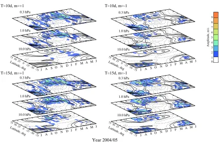
Fig. 3. The amplitudes of the MetO EW wind oscillations with periods 10 (the upper row) and 15 (the bottom row) days and
west-ward/eastward wave numbers +/−1 versus latitude are shown for the time interval from July 2004 until June 2005. The mean zonal EW
winds smoothed over 30 day intervals with 5 day step are contoured by solid (positive, eastward) and dashed (negative, westward) lines. The
thick line is the “zero wind” line. The other contours are . . .−30,−10, +10, +30... m/s.
for the first part of the winter. However, the last enhance-ments of the two waves, in late February, coincide.
The amplitudes for several horizontally propagating oscil-lations (PW) with different periods (T) and zonal wave num-bers (m) were calculated from MetO zonal winds using the least-square fitting process. Figure 3 demonstrates the ampli-tudes of eastward (m=−1) and westward (m=+1) propagat-ing waves with periods 10 and 15 days for three heights 10, 1 and 0.3 hPa. As discussed in (Chshyolkova et al., 2006), the eastward waves are baroclinic and westward are normal modes (Andrews et al., 1987). The solid and dashed lines in-dicate eastward and westward zonal mean winds, which are smoothed over 30-day intervals with a 5-day time-step. The thick solid line is the “zero-wind” line, and the step between contours is 10 m/s. Notice that the winter months of the NH are in the middle of each rectangle. It is seen from the fig-ure that in the NH the eastward waves are more active in the beginning of the winter when the eastward mean winds are strongest, and are confined to the winter hemisphere (east-ward background flow). Activity of the west(east-ward waves of the NH increases by the end of the winter, and they pene-trate to the SH in March. In October the cross-hemispheric coupling of the westward waves is somewhat smaller than in the Arctic spring (March). Compared to winters of 2000 and
2001, the amplitudes of the waves are∼1.5 times weaker this year (Chshyolkova et al., 2006).
Fig. 4. Representation of the polar vortex (blue) and anticyclones
(orange) fromθ=500 to 2000 K (∼20–50 km) isentropic surface on
25 December 2004; 1 January, 1 February and 25 February 2005.
then occupied larger areas. The strongest disturbance for this winter occurred at the end of February. For example the vor-tex structure for 25 February is demonstrated in the bottom right corner of Fig. 4. In the lower stratosphere the polar vor-tex splits into two parts, while at the upper levels the vorvor-tex is just strongly elongated and displaced from the pole. Again, the whole structure is elongated and rotated westward with height.
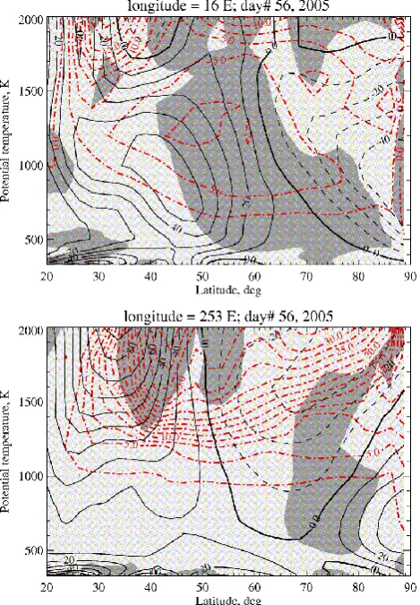
Zonal asymmetry of the winter circulation is obvious dur-ing the disturbed days, but there are also longitudinal pe-culiarities when the vortex is relatively strong and circular. This is clearly seen from the comparison of the latitude-altitude cross-sections for 253◦E (North America) and 16◦E (Scandinavia-Europe) that are shown for 25 December 2004 (Fig. 5a) and for 25 February 2005 (Fig. 5b). These plots demonstrate the Q parameter (dark/light grey shadings), “scaled” (see below) Potential Vorticity (PV, dot-dashed lines), and zonal winds (solid and dashed lines) for 20◦N– 90◦N latitudes and from 20 to 50 km heights. The areas dominated by rotation (negative Q values) are shaded with darker grey color. Eastward and westward winds are plotted using solid and dashed lines, respectively, and the thick solid lines denote the “zero-wind” line. The PV was modified by scaling it with a dimensionless factor,θ420
−4
, to remove
altitudinal dependence due to the potential temperature (θ) changes with height (M¨uller and G¨unther, 2003, 2005).
The Arctic polar vortex is clearly visible as a region bounded by closely spaced dot-dashed lines (large gradients of scaled PV in Fig. 5); it is centered almost over the pole and occupies a large area (up to∼40–50◦N). As can be seen in Fig. 5a, during December the cyclonic rotation is dominant over Europe (the top panel) at latitudes poleward of 55–60◦ with the maximum latitudinal gradients of PV also occur-ring near 55◦. In contrast, over North America (the bottom panel) there is a zone of positiveQ(“shear zone”) at∼55◦ between the central (∼60–90◦N) and mid-latitudinal (40– 50◦N) parts of the cyclonic vortex. Also notice the strong lat-itudinal gradients in PV near 40 and 55◦latitudes. Although the eastward winds demonstrate similarly very strong speeds (∼90 m/s) near the “edge” of the vortex in both meridional cross-sections, positions of the maxima are different. Maxi-mum winds are reached at∼50◦N over Europe and∼40◦N over the North American continent.
Figure 5b shows that even more differences exist between European and North American locations on 25 February, dur-ing the strongest disturbance for this winter. At the North American longitude (253◦E) a westward wind cell centered near 70◦occupies the middle to high latitudes at stratospheric levels, and the eastward wind-jet is shifted equatorward (cen-tered near 30◦N) and upward. At the same time, at the Eu-ropean longitude (16◦E), the eastward winds are still strong (∼60 m/s) and maximize near 50◦N. This is due to the defor-mation and shift of the vortex away from the pole. The part of the vortex over North America weakened, while its second part over Europe was still strong.
5 Stratosphere-mesosphere coupling
In this section analysis of winds in the height region from
Fig. 5a. Latitude-altitude cross sections of the Q parameter (dark
grey is negative, light grey is positive) at 16◦E (top) and 253◦E
(bottom) longitudes on 25 December 2004 (day number 360). Solid and dashed lines are positive (eastward) and negative (westward) MetO zonal winds (m/s), respectively. Dash-dot lines are contours
of modified PV (1PV unit=10−6m2Ks−1kg−1).
of the means. For the sake of continuity, the middle alti-tudinal section shows daily winds calculated using the ther-mal wind equation with the MetO winds at the low bound-ary (0.1 hPa). A simple linear fit was employed to calcu-late latitudinal temperature gradients from Aura MLS daily measurements within±10◦in latitude and±12◦in longitude
over the stations.
The different datasets agree well near both their bound-aries: 55 and 82 km. Good agreement is expected around 55 km as we use MetO winds at its highest levels to begin the calculation of the wind field above (55–80 km). Around
∼82 km discrepancies can be found between winds calcu-lated using thermal wind equation and radar measurements. There are several possible reasons for these discrepancies:
– There are unknown tidal signatures in Aura data. Two adjacent tracks 12 h apart have been used in calcula-tions, so the 24-h tide is minimized, while
contamina-Fig. 5b. The same as contamina-Fig. 5a only for 25 February 2005 (day num-ber 56).
tion due to the stronger 12-h tide at these latitudes could be significant. The radar winds (82–97 km) are “tidally corrected” (evidence for this is provided below). – The thermal wind equation assumes geostrophic
bal-ance (no drag), which is rarely the case in the atmo-sphere. For example, at mesospheric heights the drag due to GW and PW is strong enough (e.g. Liu and Roble, 2002) to break this assumption. Without drag the zonal winds would continue to become more east-ward throughout the 55–80 km height interval (Manson et al., 1991).
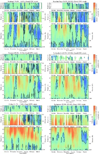
[image:9.595.311.546.64.402.2]Fig. 7. Evolution of zonal winds in the height range from the surface of the Earth up to the upper mesosphere (97 km) in the time interval from October of 2004 until March of 2005 for Tromsø and Saskatoon. The MetO daily winds are shown in the bottom panel of each plot
(0–55 km), while in the middle (55–82 km) and the top (82–97 km) panels day-time mean (≥7 h of data) centred on noon and obtained from
measurements only cover up to 82◦N. (An example of
this is shown later in Fig. 8.)
– As was mentioned in Sect. 2.3, Aura MLS temperature data are less accurate at the upper levels (0.001 hPa), although the MF radars have minimal zonal speed bias at 82 km (Sect. 2.1). Note also that there is a 2 km gap between the datasets.
– Data have different resolutions: 3 days in the 82–97 km and 1 day in the 55–82 km height regions.
The availability of the MFR data (Tromsø, Saskatoon, and Platteville) at low heights allows comparisons between direct wind measurements and the winds calculated from the ther-mal wind equation. Figure 7 presents the zonal wind time-altitude cross-section for Tromsø and Saskatoon locations in a fashion similar to Fig. 6. The lowest parts of the plots (0– 55 km) are the same in both figures and present the MetO as-similated daily zonal winds, while at the middle (55–82 km) and upper (82–97 km) heights the mean day-time winds are shown in Fig. 7. These winds were constructed from hourly data and with at least 7 values per day centered on noon. Usually, due to the increased noise level and lack of useful radar scatter during the night below∼70 km, the coverage is poorest at low heights, but becomes better near and above 80 km, where the number of hourly mean values approaches 24 (Luo et al., 2002). The averaging over 7 h minimizes GW influences.
There is very good overall qualitative agreement between calculated and measured winds (middle panels) at all three stations (Platteville is not shown). The largest differences in the middle panel occur near 80 km, where radar data of-ten show westward (blue) winds. This can be attributed to tidal contamination. The comparison of the top panels in Figs. 6 and 7 for corresponding stations also reveals that the differences are mostly due to tides (the effect of differ-ent temporal resolution is insignificant). For example, for Saskatoon (Fig. 6, bottom left panel), in October the fitted mean winds (no tidal contamination) show westward cells closing at∼82 km, while in Fig. 7 (bottom plot) the west-ward winds penetrate below∼80 km. Again, remember to keep in mind that the thermal winds are available only up to 0.001 hPa (∼80 km), while the radars have no altitudinal gaps in this region. Another factor that would contribute to the discrepancies of Figs. 6 and 7 is the geostrophic assump-tion. The GW drag is important at the mesospheric heights and, as mentioned above, acts to decrease eastward winds. The geostrophic balance assumes zero drag, so the winds cal-culated using the thermal wind equation may be more east-ward than the actual winds, especially at the upper levels. The smaller radar amplitudes could also be explained by the MF speed bias of∼20% (Sect. 2.1). Despite all these differ-ences the calculated thermal winds are a good approximation of the real winds in this height region and can be used for qualitative comparisons and wave analysis purposes.
Returning to consideration of Fig. 6, the main feature com-mon to all stations is the eastward jet (green-red colors in Fig. 6) in the stratosphere-mesosphere height region (20– 90 km), which is often referred as the polar night jet (PNJ). The maximum of the eastward flow, which is located at∼55– 60 km in early winter, decreases in magnitude and progresses downward to∼30–40 km with time. The magnitude of the PNJ varies throughout the winter with occasional reversals (blue) to the westward direction. After each disturbance, winds are restored to their normal winter values until they finally became westward throughout the middle atmosphere, marking the transition to the summer-like wind pattern. Al-though the general scenario is common for all stations, it dif-fers in detail because the radars have different locations rel-ative to the vortex. The eastward winds are weaker at higher latitudes as was also seen in Figs. 5a, b. The strong west-ward events seen at the high latitude Svalbard station below
∼85 km are much weaker at Tromsø, and are seen only as rel-atively small decreases in eastward winds at Collm. Similar latitudinal differences can be seen for Canadian stations. Sta-tions at Andenes, Esrange (not shown), and Tromsø are rela-tively close (125–270 km), and zonal wind time-variations at these stations are quite similar.
Longitudinal variations are apparent between Collm and Saskatoon (bottom plots in Fig. 6). The eastward winds are weaker at Saskatoon, which can be explained by the different location of the PNJ maximum over Europe and North America: 50◦N for 16◦E longitude and near 40◦N for 253◦E (Fig. 5). Indeed, the wind contours for Platteville (not shown) do exhibit much stronger eastward flows than at Saskatoon, which persist above ∼40 km throughout all winter until the end of March. Also, at the end of Febru-ary (warming event) the transition to the westward winds oc-curred over Saskatoon between 20 and 97 km, while at Collm the westward wind cell occupies the region between ∼40 and 80 km for a few days, with eastward winds at heights near 30 km until the end of March. This reflects the vortex characteristics during this time (Sect. 4, bottom left plot in Fig. 4), and is consistent with Fig. 5b that shows weak west-ward winds at stratospheric levels for latitudes higher than 50◦N (bottom plot) for Saskatoon longitudes, while there are still quite strong (∼60 m/s) eastward winds over Europe at 50◦N (top plot). Obninsk is located at a similar latitude, but is∼20◦east of Collm. Zonal winds at Obninsk (not shown) are similar to those at Collm station, except they were less westward in the 55–82 km height range at the end of Jan-uary/beginning of February. The meteor radar at Obninsk does not provide height information, and all reflections are assumed to be from the height region centered at approxi-mately 94 km. These winds and Collm winds at 94 km agree well, and have such similarities as wind reversals in the mid-dle of January, the beginning of February, and in the midmid-dle of March.
Scandinavian-European and Canadian stations. For example, the PNJ has stronger magnitudes at Poker Flat (∼65◦N) than
at Canadian/European stations with similar latitudes. Over Wakkanai the first strong westward reversal occurred in the first half of January between 20 and 70 km, and was fol-lowed by the second stronger reversal in February. Later the winds became weakly eastward above∼40–50 km, but re-mained westward in the lower stratosphere until the end of the March. These may be explained by the relatively close proximity of these stations to the Aleutian High.
Continuing with perusal of Fig. 6, in the upper meso-spheric region (82–97 km) the eastward zonal winds decrease in magnitude with increasing height at all stations, although their particular variations differ. Most of their variability can probably be explained by the local effects of GWs on the mean flow (deceleration of the flow as well as induced vari-ability with periods in the PW range, see for example Smith, 1996). Some of the reversals of the eastward mesospheric winds can be linked to the wind reversals below. The warm-ing event at the end of February is the best example of such connection between mesosphere and stratosphere. The tim-ing of such reversals appears to be approximately the same throughout the whole height range or sometimes a little ear-lier at the upper altitudes.
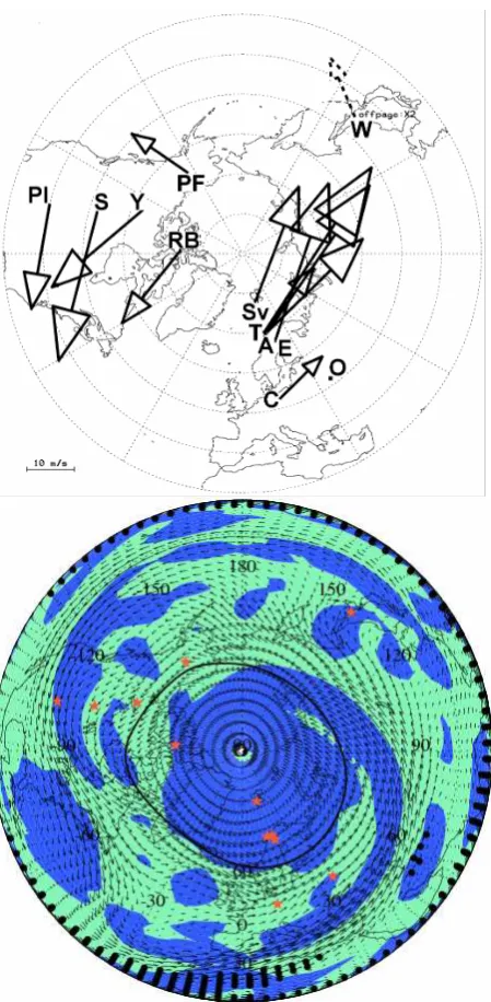
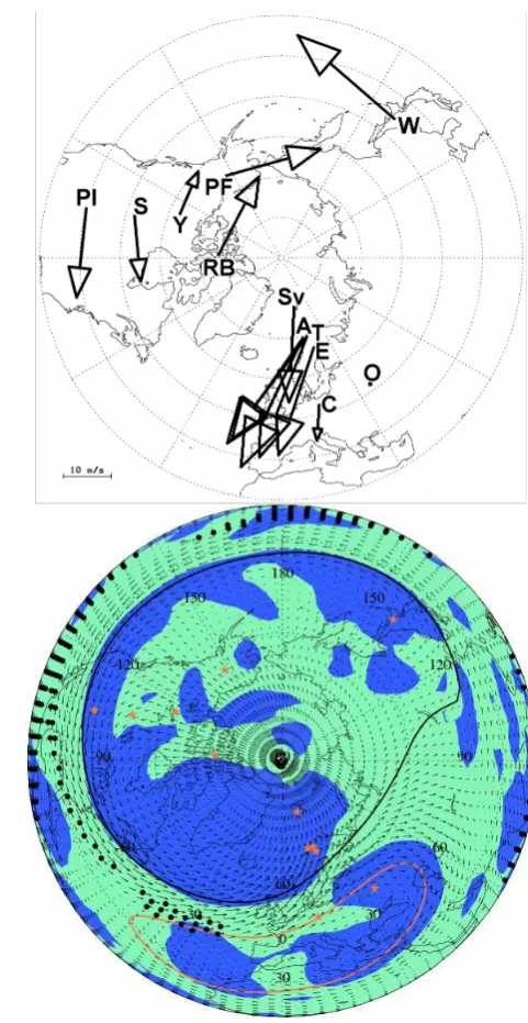
Next, an attempt to compare winds from the upper strato-spheric (∼50–60 km) heights with those from the meso-spheric heights (82 km) is made with the emphases on the vortex structure rather than consideration of eastward wind profiles at separate locations. The comparison is difficult mostly due to the lack of mesospheric observations. All available 3-day radar vectors were inspected. Days that in-dicated the usual winter cyclonic flow around the pole and events in February (1 and 19) were chosen for demonstra-tion. In Fig. 8 the daily MetO winds at 2000 K (∼50 km) isentropic surface (lower plots) along with the 3-day mean wind vectors (82 km) obtained at 12 radar stations (upper plots) are shown for 20 January, 1, 13, and 19 February 2005. The lower plots are the stereographic projections (15–90◦N) of the Q-diagnostic over the NH with the blue areas where Q is negative (rotation dominates the flow) and green ar-eas where Q is positive (strain is dominant). Black arrows are winds, red stars are locations of the radar stations, and black/red lines are estimated edges of cyclones/anticyclones. Black filled dots are assigned to the areas with the negative PV, which are usual at low latitudes. Sometimes, however, the black dots can be found more poleward, which indicates an intrusion of the tropical air to the mid-latitudinal region at the upper stratospheric heights (Harvey et al., 2002). The vortex plots are daily, while the radar winds are obtained over 3-day interval centered on the chosen dates.
First of all at the upper stratospheric heights the vortex does not have the “solid” or continuous shape as it usually has in the middle stratosphere; at these levels patches of blue color are scattered over the hemisphere composing some kind of spiral or comma shapes. The meridional wind
com-ponent is often strong, and there is, therefore, significant di-vergence from the cyclonic eastward flow. On the upper plots vectors of the mesospheric mean wind measured at 12 loca-tions (the same localoca-tions that are shown by red stars on the lower plots) are placed on top of the stereographic map (30– 90◦N). In January (e.g. 20 January, Fig. 8a) arrangement of radar wind vectors is consistent with cyclonic motion around the pole, and they match well the MetO winds at correspond-ing locations. Often, especially when negative areas of Q have consistent large circular shapes with little or no shear (green) zones inside, the stratospheric and mesospheric vec-tors show very close similarity in their directions. Usually best agreement requires a shift of the vortex with height, for example.
On 1 February (Fig. 8b), the time of the weak strato-spheric disturbance, radar and MetO wind vectors over high-latitudinal stations (>60◦N) demonstrate opposite directions
and have strong meridional components. This suggests an existence of strong thermal gradients of opposite directions at stratospheric and mesospheric heights. The MetO data at ∼30 km (not shown) indicate that the polar vortex was squeezed by two anticyclones located at lower latitudes in the 330–360◦E and 90–180◦E longitudinal sectors. The stronger of the two anticyclones (90–180◦E) also pushed the polar vortex away from the pole, which is reflected in Fig. 2 as amplitude of SPW1 increases at 60◦N. Therefore the boundary between cold and warm regions lay across the pole, and strong poleward/equatorward flows were es-tablished in the 30–60◦E and 210–240◦E longitudinal seg-ments, respectively (Fig. 8b). At the upper heights (layer 50–80 km) the Aura measurements (not shown) indicate re-versed temperature gradients (cold in 120◦E sector), so that
winds at∼80 km, through thermal wind equation, now have opposite directions to the stratospheric winds. The winds were weak over Canadian stations (Platteville, Saskatoon, and Yellowknife), which are situated farther from this region of strong temperature gradients.
Fig. 8a. Evolution of the daily MetO winds (black arrows) at 2000 K isentropic surface (bottom) and 3-day mean winds obtained at 12 radar locations (82 km, top) for 20 January 2005. The dashed arrow indicates the speed is twice as big as that shown.
mesospheric heights, which can explain the more diverse re-lationships between stratospheric and mesospheric winds de-pending on the locations.
Finally by 25 February the vortex was split in two uneven parts at low stratospheric heights with the stronger part being over Europe (Fig. 4, bottom right). In the upper stratosphere (not shown) the vortex was deformed and twisted westward with height, so that the stronger cyclonic area was located over North America. At mesospheric heights (not shown)
Fig. 8b. The same as Fig. 8a, but for 1 February 2005.
winds were also weak and completely disorganized. Later in March the cyclonic flow was partially restored at 50 and 82 km, before it disappeared during the transition to the sum-mer circulation.
[image:14.595.314.542.63.515.2]Fig. 8c. The same as Fig. 8a, but for 13 February 2005.
of the winds with height. This is in agreement, through the thermal wind equation, with a warm mesopause region, which is normal in winter. However at the end of February, during the strongest, for this winter, stratospheric disturbance the difference-vectors at these stations (except Platteville, a more equatorward station) are smaller or eastward (pointed to the right). This indicates weakening or reverse of the east-ward flow in the stratopause.
Significant deviation of the illustrated strong difference-vectors from the horizontal line (EW direction) implies re-versed meridional flow between the ∼64 km and 82 km heights. The downward (in the figure) or southward
direc-Fig. 8d. The same as direc-Fig. 8a, but for 19 February 2005.
[image:15.595.64.329.61.521.2]Differences between vectors "radar 82km"-"MetO ~64km"
0 5 10 15 20 25 30
December, 2004 Poker Flat
Wakkanai Platteville Saskatoon Yellowknife Resolute Bay Svalbard Tromso Andenes Esrange Obninsk Collm
150 m/s
Differences between vectors "radar 82km"-"MetO ~64km"
0 5 10 15 20 25 30
January, 2005 Poker Flat
Wakkanai Platteville Saskatoon Yellowknife Resolute Bay Svalbard Tromso Andenes Esrange Obninsk Collm
150 m/s
Differences between vectors "radar 82km"-"MetO ~64km"
0 5 10 15 20 25 30
February, 2005 Poker Flat
Wakkanai Platteville Saskatoon Yellowknife Resolute Bay Svalbard Tromso Andenes Esrange Obninsk Collm
[image:16.595.51.285.62.371.2]150 m/s
Fig. 9. Vectors of differences between radar winds measured at
82 km and MetO assimilated winds at∼64 km for 3 months of
win-ter of 2004/05 (December, January, and February) for 12 locations.
are also close together and located inside the vortex, the an-gles of their difference-vectors do not always change simi-larly with time. However, the difference-vectors are predom-inantly northward, consistent with southward stratopause winds, for both stations. The angles, therefore, differ from those at Scandinavian stations. The difference-vectors at the Poker Flat and Wakkanai locations exhibit their own patterns of angle variations, which have strong northward compo-nents, especially at Poker Flat (a more poleward location). The longitudinal variations in the difference-vectors are due to the distortions of the vortex and/or its movement off the pole.
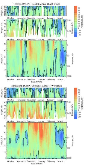
To study the wind variability with periods from 2 to 30 days, the Morlet wavelet (Torrence and Compo, 1998) has been employed. Figure 10 demonstrates examples of wavelet amplitudes of the MetO (∼50 km, left column) and Radar (82 km, right column) zonal winds for Svalbard, Tromsø, Collm, and Saskatoon (from the top to the bottom). The black line indicates areas with 90% significance. The three Scandinavian-European stations have similar spectra: long periods (>20 days) in November, short periods (less than 5 days) through out the most of the winter, and energy for pe-riods between 4 and 20 days at the end of February. Clearly
there are some differences in exact locations of the peaks as well as their amplitudes, which are smaller at more poleward stations. Some of these differences could be due to differ-ent propagation conditions for the PW at these three stations. As can be seen in Fig. 6, at the end of February the westward background winds are stronger below 50 km at Svalbard than at Tromsø, while over Collm the winds have eastward direc-tions. PW propagation is favored by eastward winds of mod-erate magnitude (Andrews et al., 1987). Wavelets of MetO zonal winds at Saskatoon have overall smaller amplitudes. Similar to the other stations there is energy at longer peri-ods in November, but in the middle of February there is only one relatively weak peak around 8 days and 10-day maxima appears in the first half of March. This is consistent with the zero wind line and the cell of westward winds at strato-spheric heights over, and northward of, Saskatoon (Fig. 5b), which will favor refraction of PW to lower latitudes. The wavelets at the mesospheric heights (the right column) have much smaller amplitudes and do not have many similarities. This variability of local PW activity (latitudinally and longi-tudinally) is consistent with the earlier study of 16-day PW activity provided by (Luo et al., 2002). In general, com-pared to previous years, the winter of 2004/05 is charac-terized by weak planetary wave activity at stratospheric and mesospheric heights.
6 Summary
The evolution of the polar vortex during the Arctic winter of 2004/05 has been studied using MetO assimilated fields and data from meteor and MF radars at 12 mid- and high-latitude locations. The winter of 2004/05 was shown to be rela-tively cold with no major mid-winter stratospheric warmings. MetO parameters near 32 km averaged over 60◦N and 70◦N latitudinal circles exhibit neither rapid temperature increases of 25◦K or more, nor corresponding reversal of the zonal winds. However there were 3 time intervals with increasing northern temperatures and corresponding weakening of the zonal winds: the end of December/beginning of January, the end of January/beginning of February, and the end of Febru-ary. During the first two intervals the disturbances were rel-atively weak. The event at the end of February was the fi-nal and strongest disturbance for this winter, and marked the beginning of the wind transition toward summer-like circula-tion.
EW (MetO) 0.46 hPa
Nov Dec Jan Feb Mar 0
5 10 15 20 25 30
PERIOD (day) 90% 90%
EW (Radar) 82 km
Nov Dec Jan Feb Mar 0
5 10 15 20 25 30
90%
90%
Svalbard
Nov Dec Jan Feb Mar 0
5 10 15 20 25 30
PERIOD (day)
90%
90%
Nov Dec Jan Feb Mar 0
5 10 15 20 25 30
90% Tromso
Nov Dec Jan Feb Mar 0
5 10 15 20 25 30
PERIOD (day)
90%
90%
90%
Nov Dec Jan Feb Mar 0
5 10 15 20 25 30
Collm
Nov Dec Jan Feb Mar 2004/05
0 5 10 15 20 25 30
PERIOD (day)
90% 90%
Nov Dec Jan Feb Mar 2004/05
0 5 10 15 20 25 30
90% 90%
Saskatoon
0 2 4 6 8 10 12 14 16 18 20 Amplitude, m/s
[image:17.595.130.469.61.493.2]
Fig. 10. Wavelet amplitudes versus time (November 2004–March 2005) and period (2–30 days) calculated for the zonal wind component of the MetO winds at 0.46 hPa (left column) and of radar measurements at 82 km (right column) for the Svalbard, Tromsø, Collm, and Saskatoon locations.
upper stratospheric levels. The eastward propagating waves had maxima in the early winter and were confined to the areas with eastward wind flow, consistent with baroclinic waves. The amplitudes of the westward propagating waves (normal modes) increased by the end of winter (February) and were reaching Southern Hemispheric latitudes at upper stratospheric levels in March. Both eastward and westward amplitudes were∼1.5 times smaller than those calculated for years 2000 and 2001 (Chshyolkova et al., 2006).
To study the longitudinal variations of the polar vortex, the Q-diagnostic was used to characterize the dynamics of the middle and upper stratosphere. The results show that the NH polar vortex formed in mid-autumn, and was fully
estab-lished by 1 December 2004. In December the polar vortex reached its strongest state: it was centered on the pole and occupied a relatively large area. During the three disturbed time intervals the vortex was elongated, slightly shifted off the pole, had a westward tilt with height, and had decreased areas in the lower stratosphere. The deformations were the largest for the last event, when the vortex was divided in two unequal parts below∼600 K isentropic (∼24 km) level.
∼50◦N) than over North America (at∼40◦N). During the
late February disturbance the largest differences in the lower and middle stratosphere were between stations located near 50◦N latitude: Saskatoon (253◦E) and Collm (13◦E). The part of the vortex over Europe was stronger and eastward winds continued to be observed at Collm. In contrast, over Canada winds were westward, as the smaller part of the vor-tex was practically destroyed and the eastward jet was shifted upward and equatorward. The wavelet amplitudes for the stratospheric PW oscillations with periods from 2 to 30 days were also remarkably different between European and North American sectors. All stations demonstrated strong activity with periods longer than 20 days in November and an ab-sence of oscillations with periods longer than∼5 days in the middle of winter. In February, though, wavelet analysis indi-cated lower PW activity at Saskatoon compared to Collm.
Strong latitudinal differences were also apparent in the zonal wind contour plots and wavelet amplitudes. The east-ward winds were systematically weaker and amplitudes of the oscillations associated with PW were smaller at more poleward stations.
Compared to the stratospheric winds, the wavelets of the EW component indicated that the PW had smaller ampli-tudes and did not show many similarities between stations in the mesosphere. In general, compared to previous years, the winter of 2004/05 could be characterized by weak planetary wave activity at stratospheric and mesospheric heights.
This study suggests that analyses of wind fields at strato-spheric and mesostrato-spheric heights should not assume that os-cillations with periods of days (5–20), which are normally as-sociated with PW activity, exhibit similar amplitude variabil-ities at all longitudes, i.e. that zonal wave number analysis of global data (model or satellite) for a single mode may pro-duce inaccurate wave characteristics. This variation of PW would be expected when the polar vortex is not centered on the pole and/or is elongated (not circular in shape). Thus this study expands and validates earlier studies (Luo et al., 2002; Manson et al., 2004, 2006) on winter time PW characteris-tics. A continuation of this study will include chemicals (O3,
N2O, HCl, and ClO) from Aura and will illustrate the effects
of vortex elongation and displacement. The use of equivalent latitudes (e.g. Manney et al., 2006) helps to deal with vortex displacement issues, but not the elongation. The existence of asymmetry, which results from both of these characteristics, has led to the extreme variability in longitudinal dynamical characteristics shown in this study for 2004/05.
Acknowledgements. The authors would like to express their
grat-itude to V. L. Harvey and T. D. Fairlie for their help with the Q-diagnostic. T. Chshyolkova is grateful to E. Merzlyakov for his comments. Thanks are due to the Aura team for their MLS dataset as well as to the UK Meteorological Office for the stratospheric assimilated data and to the British Atmosphere Data centre for pro-viding access to these data. The authors are also thankful to the referees for their comments and questions.
Topical Editor U.-P. Hoppe thanks G. G. Shepherd and D. Pancheva for their help in evaluating this paper.
References
Andrews, D. G., Holton, D. G., and Leovy, C. B.: Middle Atmo-sphere Dynamics, Academic Press, 489 pp., 1987.
Babiano, A., Boffetta, G., Provenzale, A., and Vulpiani, A.: Chaotic advection in point vortex models and two-dimensional turbu-lence, Phys. Fluids, 6(7), 2465–2474, doi:10.1063/1.868194, 1994.
Bhattacharya, Y., Shepherd, G. G., and Brown, S.: Variability of atmospheric winds and waves in the Arctic polar mesosphere during a stratospheric sudden warming, Geophys. Res. Lett., 31, L23101, doi:10.1029/2004GL020389, 2004.
Briggs, B. H.: The analysis of spaced sensor records by correlation techniques, in: International Council of Scientific Unions Middle Atmosphere Program, 13, 166–186, 1984.
Cervera, M. A. and Reid, I. M.: Comparison of simultaneous wind measurements using collocated VHF meteor radar and MF spaced antenna radar systems, Radio Sci., 30(4), 1245–1262, 1995.
Chshyolkova, T., Manson, A. H., Meek, C. E., Avery, S. K., Thorsen, D., MacDougall, J. W., Hocking, W., Murayama, Y., and Igarashi, K.: Planetary wave coupling in the middle atmo-sphere (20–90 km): A study involving TOMS, MetO and MF radar data, Ann. Geophys., 23, 1103–1131, 2005,
http://www.ann-geophys.net/23/1103/2005/.
Chshyolkova, T., Manson, A. H., Meek, C. E., Avery, S. K., Thorsen, D., MacDougall, J. W., Hocking, W., Murayama, Y., and Igarashi, K.: Planetary wave coupling processes in the mid-dle atmosphere (30–90 km): A study involving MetO and MFR data, J. Atmos. Solar-Terr. Phys., 68(3–5), 353–368, 2006.
Fairlie, T. D. A.: Three-dimensional transport simulations
of the dispersal of volcanic aerosol from Mount Pinatubo,
Quart. J. Roy. Meteorol. Soc., 121(528), 1943–1980,
doi:10.1256/smsqj.52808, 1995.
Froidevaux, L., Livesey, N. J., Read, W. G., Jiang, Y. B, Jimenez, C. C., Filipiak, M. J., Schwartz, M. J., Santee, M. L., Pumphrey, H. C., and Jiang, J. H.: Early validation analyses of atmospheric profiles from EOS MLS on the Aura satellite, IEICE T. Com-mun., 44(5), 1106–1121, 2006.
Gregory, J. B. and Manson, A. H.: Winds and wave motions to 110 km at mid-latitudes. III Response of mesospheric and ther-mospheric winds to major stratospheric warmings, J. Atmos. Sci., 32(9), 1676–1681, 1975.
Greisiger, K. M., Portnyagin, Y. I., and Lyssenko, I. A.: Large-scale winter-time disturbances in meteor winds over Central and Eastern Europe and their connection with processes in the strato-sphere, J. Atmos. Terr. Phys., 46(4), 389–394, 1984.
Hall, C.: The Ramfjordmoen MF radar (69◦N, 19◦E): application
development 1990–2000, J. Atmos. Solar-Terr. Phys., 63(2–3), 171–179, 2001.
Hall, C. M., Aso, T., Manson, A. H., Meek, C. E., Nozawa, S., and Tsutsumi, M.: High-latitude mesospheric mean winds: A com-parison between Tromsø (69 N) and Svalbard (78 N), J. Geophys. Res., 108(D19), 4598, doi:10.1029/2003JD003509, 2003. Hall, C. M., Aso, T., Tsutsumi, M., Nozawa, S., Manson,
lower thermosphere neutral winds as determined by meteor and
medium-frequency radar at 70◦N, Radio Sci., 40(4), RS4001,
doi:10.1029/2004RS003102, 2005.
Harvey, V. L., Pierce, R. B., Fairlie, T. D., and Hitchman, M. H.: A climatology of stratospheric polar vortices and anticyclones, J. Geophys. Res., 107(D20), 4442, doi:10.1029/2001JD001471, 2002.
Hocking, W. K., Fuller, B., and Vandepeer, B.: Real-time deter-mination of meteor-related parameters utilizing modern digital technology, J. Atmos. Solar-Terr. Phys., 63(2–3), 155–169, 2001. Hocking, W. K.: Experimental Radar Studies of Anisotropic Diffu-sion of High Altitude Meteor Trails, Earth Moon Planets, 95(1), 671–679, 2004.
Hoffmann, P., Singer, W., and Keuer, D.: Variability of the meso-spheric wind field at middle and Arctic latitudes in winter and its relation to stratospheric circulation disturbances, J. Atmos. Solar-Terr. Phys., 64(8–11), 1229–1240, 2002.
Holton, J. R.: The Influence of Gravity-Wave Breaking on the General-Circulation of the Middle Atmosphere, J. Atmos. Sci., 40(10), 2497–2507, 1983.
Jacobi, C., Schminder, R., and K¨urschner, D.: The winter
mesopause wind field over Central Europe and its response to stratospheric warmings as measured by LF D1 wind measure-ments at Collm, Germany, Adv. Space Res., 20(6), 1223–1226, 1997.
Jacobi, C., K¨urschner, D., Muller, H. G., Pancheva, D., Mitchell, N. J., and Naujokat, B.: Response of the mesopause region dy-namics to the February 2001 stratospheric warming, J. Atmos. Solar-Terr. Phys., 65(7), 843–855, 2003.
Jacobi, C., K¨urschner, D., Fr¨ohlich, K., Arnold, K., and Tetzlaff, G.: Meteor radar wind and temperature measurements over Collm (51.3 N, 13 E) and comparison with co-located LF drift mea-surements during autumn 2004, Reports Inst. Meteorol. Univ. Leipzig, 36, 98–112, 2005.
Jim´enez, C., Pumphrey, H. C., MacKenzie, I. A., Manney, G. L., Santee, M. L., Schwartz, M. J., Harwood, R. S., and
Wa-ters, J. W.: EOS MLS observations of dehydration in the
2004-2005 polar winters, Geophys. Res. Lett., 33(16), L16806, doi:10.1029/2006GL025926, 2006.
Labitzke, K.: Temperature changes in the mesosphere and strato-sphere connected with circulation changes in winter, J. Atmos. Sci., 29(4), 756–766, 1972.
Lindzen, R. S.: Turbulence and stress owing to gravity wave and tidal breakdown, J. Geophys. Res., 86, 9707–9714, 1981. Liu, H. L. and Roble, R. G.: A study of a self-generated
strato-spheric sudden warming and its mesostrato-spheric-lower thermo-spheric impacts using the coupled TIME-GCM/CCM3, J. Geo-phys. Res., 107(D23), 4695, doi:10.1029/2001JD001533, 2002. Lorenc, A. C., Ballard, S. P., Bell, R. S., Ingleby, N. B., Andrews,
P. L. F., Barker, D. M., Bray, J. R., Clayton, A. M., Dalby, T., Li, D., Payne, T. J., and Saunders, F. W.: The Met. Office global three-dimensional variational data assimilation scheme, Quart. J. Roy. Meteorol. Soc., Part B, 126(570), 2991–3012, 2000. Luo, Y., Manson, A. H., Meek, C. E., Meyer, C. K. Burrage, M.
D., Fritts, D. C., Hall, C. M., Hocking, W. K., MacDougall, J., Riggin, D. M., and Vincent, R. A.: The 16-day planetary waves: multi-MF radar observations from the arctic to equator and comparisons with the HRDI measurements and the GSWM modelling results, Ann. Geophys., 20, 691–709, 2002,
http://www.ann-geophys.net/20/691/2002/.
Manney, G. L., Santee, M. L., Froidevaux, L., Hoppel, K., Livesey, N. J., and Waters, J. W.: EOS MLS observations of ozone loss in the 2004–2005 Arctic winter, Geophys. Res. Lett., 33(4), L04802, doi:10.1029/2005GL024494, 2006.
Manson, A. H., Gregory, J. B., and Stephenson, D. G.: Winds and wave motions /70–100 km/ as measured by a partial reflection radiowave system, J. Atmos. Terr. Phys., 35, 2055–2067, 1973. Manson, A. H., Meek, C. E., Fleming, E., Chandra, S., Vincent,
R. A., Phillips, A., Avery, S. K., Fraser, G. J., Smith M. J., and Fellous, J. L.: Comparisons between Satellite-derived Gradient Winds and Radar-derived Winds from the CIRA-86, J. Atmos. Sci., 48(3), 411–428, 1991.
Manson, A. H., Meek, C. E., Stegman, J., Espy, P. J., Roble, R. G., Hall, C. M., Hoffmann, P., and Jacobi, Ch.: Springtime transition in mesopause airglow and dynamics: photometer and MF Radar observations in the Scandinavian and Canadian sectors, J. Atmos. Solar-Terr. Phys. 64, 1131–1146, 2002.
Manson, A. H., Meek, C. E., Avery, S. K., and Thorsen, D.: Iono-spheric and dynamical characteristics of the mesosphere-lower
thermosphere region over Platteville (40◦N, 105◦W) and
com-parisons with the region over Saskatoon (52◦N, 107◦W), J.
Geo-phys. Res., 108(D13), 4398, doi:10.1029/2002JD002835, 2003. Manson, A. H., Meek, C. E., Chshyolkova, T., Avery, S. K.,
Thorsen, D., MacDougall, J. W., Hocking, W., Murayama, Y., Igarashi, K., Namboothiri, S. P., and Kishore, P.: Longitudinal and latitudinal variations in dynamic characteristics of the MLT (70–95 km): a study involving the CUJO network, Ann. Geo-phys., 22, 347–365, 2004,
http://www.ann-geophys.net/22/347/2004/.
Manson, A. H., Meek, C. E., Chshyolkova, T., McLandress, C., Av-ery, S. K., Fritts, D. C., Hall, C. M., Hocking, W. K., Igarashi, K., MacDougall, J. W., Murayama, Y., Riggin, D. C., Thorsen, D., and Vincent, R. A.: Winter warmings, tides and planetary waves: comparisons between CMAM (with interactive chemistry) and MFR-MetO observations and data, Ann. Geophys., 24, 2493– 2518, 2006,
http://www.ann-geophys.net/24/2493/2006/.
Matsuno, T.: A Dynamical Model of the Stratospheric Sudden Warming. J. Atmos. Sci., 28(8), 1479–1494, 1971.
Meek, C. E.: An efficient method for analysing ionospheric drifts data, J. Atmos. Terr. Phys., 42, 835–839, 1980.
Mitchell, N. J., Pancheva, D., Middleton, H. R., and Hagan,
M. E.: Mean winds and tides in the Arctic mesosphere
and lower thermosphere, J. Geophys. Res., 107(A1), 1004, doi:10.1029/2001JA900127, 2002.
M¨uller, R. and G¨unther, G.: A generalized form of Lait’s modified potential vorticity, J. Atmos. Sci., 60(17), 2229–2237, 2003. M¨uller, R. and G¨unther, G.: Polytropic atmospheres and the scaling
of potential vorticity, Meteorol. Atmos. Phys., 90(3–4), 153–157, 2005.
Murayama, Y., Igarashi, K., Rice, D. D., Watkins, B. J., Collins, R. L., Mizutani, K., Saito, Y., and Kainuma, S.: Medium frequency radars in Japan and Alaska for upper atmosphere observations, IEICE T. Commun., E83-B(9), 1996–2003, 2000.
Portnyagin, Yu. I., Merzlyakov, E. G., Solovjova, T. V., Jacobi, Ch., K¨urschner, D., Manson, A., and Meek, C.: Long-term trends and year-to-year variability of mid-latitude mesosphere/lower ther-mosphere winds, J. Atmos. Solar-Terr. Phys., 68, 1890–1901, 2006.
Randel, W., Udelhofen, P., Fleming, E., Geller, M., Gelman, M., Hamilton, K., Karoly, D., Ortland, D., Pawson, S., Swinbank, R., Wu, F., Baldwin M., Chanin, M.-L., Keckhut, P., Labitzke, K., Remsberg, E., Simmons, A., and Wu, D.: The SPARC in-tercomparison of middle-atmosphere climatologies, J. Climate, 17(5), 986–1003, 2004.
Schoeberl, M. R. and Hartmann, D. L.: The Dynamics of the Strato-spheric Polar Vortex and its Relation to Springtime Ozone Deple-tions, Science, 251(4989), 46–52, 1991.
Shepherd, T. G.: The middle atmosphere, J. Atmos. Solar-Terr. Phys., 62(17–18), 1587–1601, 2000.
Singer, W., Keuer, D., and Eriksen, W.: The ALOMAR MF Radar: Technical Design and First Results, European Rocket and Bal-loon Programmes and Related Research, Proceedings of the 13th
ESA Symposium held 26–29 May, 1997 in ¨Oland, Sweden, 26–
29 May, 1997.
Smith, M. J., Gregory, J. B., Manson, A. H., Meek, C. E., Sch-minder, R., K¨urschner, D., and Labitzke, K.: Responses of the upper middle atmosphere (60–110 km) to the stratwarms of the four pre-map winters (1978/9–1981/2), Adv. Space Res., 2(10), 173–176, 1982.
Smith, A. K.: Longitudinal variations in mesospheric winds: ev-idence for gravity wave filtering by planetary waves, J. Atmos. Sci, 53, 1156–1173, 1996.
Thayaparan, T., Hocking, W. K., and MacDougall, J.: Middle
at-mospheric winds and tides over London, Canada (43◦N, 81◦W)
during 1992–1993, Radio Sci., 30(4), 1293–1309, 1995. Thayaparan, T. and Hocking, W. K.: A long-term comparison of
winds and tides measured at London, Canada (43◦N, 81◦W) by
co-located MF and meteor radars during 1994–1999, J. Atmos. Solar-Terr. Phys., 64(8–11), 931–946, 2002.
Torrence, C. and Compo, G. P.: A practical guide to wavelet analy-sis, B. Am. Meteorol. Soc., 79(1), 61–78, 1998.
Wallace, J. M. and Hobbs, P. V.: Atmospheric science: an introduc-tory survey, 2nd ed., Elsevier Inc, 483 pp., 2006.