Ann. Geophys., 31, 1251–1265, 2013 www.ann-geophys.net/31/1251/2013/ doi:10.5194/angeo-31-1251-2013
© Author(s) 2013. CC Attribution 3.0 License.
EGU Journal Logos (RGB)
Advances in
Geosciences
Open Access
Natural Hazards
and Earth System
Sciences
Open AccessAnnales
Geophysicae
Open AccessNonlinear Processes
in Geophysics
Open AccessAtmospheric
Chemistry
and Physics
Open AccessAtmospheric
Chemistry
and Physics
Open Access DiscussionsAtmospheric
Measurement
Techniques
Open AccessAtmospheric
Measurement
Techniques
Open Access DiscussionsBiogeosciences
Open Access Open Access
Biogeosciences
DiscussionsClimate
of the Past
Open Access Open Access
Climate
of the Past
Discussions
Earth System
Dynamics
Open Access Open Access
Earth System
Dynamics
DiscussionsGeoscientific
Instrumentation
Methods and
Data Systems
Open Access
Geoscientific
Instrumentation
Methods and
Data Systems
Open Access DiscussionsGeoscientific
Model Development
Open Access Open Access
Geoscientific
Model Development
DiscussionsHydrology and
Earth System
Sciences
Open AccessHydrology and
Earth System
Sciences
Open Access DiscussionsOcean Science
Open Access Open Access
Ocean Science
DiscussionsSolid Earth
Open Access Open Access
Solid Earth
Discussions
The Cryosphere
Open Access Open Access
The Cryosphere
Natural Hazards
and Earth System
Sciences
Open Access
Discussions
On the relationship between interplanetary coronal mass ejections
and magnetic clouds
E. K. J. Kilpua1, A. Isavnin1, A. Vourlidas2, H. E. J. Koskinen1,3, and L. Rodriguez4
1Department of Physics, P.O. Box 64, University of Helsinki, Finland
2Space Science Division, Naval Research Laboratory, Washington, D.C. 20375, USA 3Finnish Meteorological Institute, P.O. Box 503, Helsinki, Finland
4Solar-Terrestrial Center of Excellence – SIDC, Royal Observatory of Belgium, Av. Circulaire 3, 1180, Brussels, Belgium
Correspondence to: E. K. J. Kilpua ([email protected])
Received: 10 January 2013 – Revised: 3 June 2013 – Accepted: 18 June 2013 – Published: 23 July 2013
Abstract. The relationship of magnetic clouds (MCs) to
in-terplanetary coronal mass ejections (ICMEs) is still an open issue in space research. The view that all ICMEs would origi-nate as magnetic flux ropes has received increasing attention, although near the orbit of the Earth only about one-third of ICMEs show clear MC signatures and often the MC occupies only a portion of the more extended region showing ICME signatures. In this work we analyze 79 events between 1996 and 2009 reported in existing ICME/MC catalogs (Wind magnetic cloud list and the Richardson and Cane ICME list) using near-Earth observations by ACE (Advanced Composi-tion Explorer) and Wind. We perform a systematic compari-son of cases where ICME and MC signatures coincided and where ICME signatures extended significantly beyond the MC boundaries. We find clear differences in the character-istics of these two event types. In particular, the events where ICME signatures continued more than 6 h past the MC rear boundary had 2.7 times larger speed difference between the ICME’s leading edge and the preceding solar wind, 1.4 times higher magnetic fields, 2.1 times larger widths and they ex-perienced three times more often strong expansion than the events for which the rear boundaries coincided. The events with significant mismatch in MC and ICME boundary times were also embedded in a faster solar wind and the major-ity of them were observed close to the solar maximum. Our analysis shows that the sheath, the MC and the regions of ICME-related plasma in front and behind the MC have dif-ferent magnetic field, plasma and charge state characteristics, thus suggesting that these regions separate already close to the Sun. Our study shows that the geometrical effect (the en-counter through the CME leg and/or far from the flux rope
center) does not contribute much to the observed mismatch in the MC and ICME boundary times.
Keywords. Solar physics, astrophysics, and astronomy
(flares and mass ejections)
1 Introduction
Coronal mass ejections (CMEs) have been intensively stud-ied for several decades because they play a key role in driving space weather to Earth (e.g., Webb et al., 2000; Huttunen et al., 2005). CMEs were discovered by the OSO-7 (Orbiting Solar Observatory) coronagraph in the early 1970s (Tousey, 1972). Later, CMEs were defined as an observable change in the coronal structure on timescales between a few min-utes and several hours, involving the appearance of a new, discrete, and bright white-light feature by Hundhausen et al. (1984). As emphasized by Schwenn (1996) this early def-inition of a CME is observational and is not based on the origin of the eruptive material nor the underlying physical processes.
Most current knowledge on the properties and struc-ture of CMEs has been derived from white-light corona-graph images (e.g., Hundhausen et al., 1984; St. Cyr et al., 2000; Cremades and Bothmer, 2004; Vourlidas et al., 2010). At present, space-based coronagraph observations come from LASCO (Large Angle and Spectrometric Coro-nagraph) (Brueckner et al., 1995) onboard SOHO (Solar and Heliospheric Observatory) and from the SECCHI (Sun– Earth Connection Coronal and Heliospheric Investigation) instrument package (Howard et al., 2008) on STEREO (Solar
Terrestrial Relations Observatory). The LASCO C3 field of view extends up to 32 solar radii (RS) from the Sun, while the outer coronagraph COR2 on STEREO views up to 15RS.
The connection between white-light and in situ distur-bances was established soon after the discovery of CMEs (e.g., Sheeley et al., 1983). Although CMEs can be now fol-lowed with heliospheric imagers (SMEI/Coriolis, Eyles et al., 2003; SECCHI/STEREO Harrison et al., 2005) to the orbit of the Earth (e.g., Tappin et al., 2004; Harrison et al., 2009), linking remote CME observations to the structure of their in situ counterparts is not straightforward. The white-light morphology is difficult to interpret as the images rep-resent a line-of-sight projection of optically thin structures and because CME emission becomes increasingly fainter the further out in the heliosphere the CME travels (e.g., Lugaz et al., 2005; Howard and Tappin, 2009; Rouillard, 2011). In turn, the majority of in situ observations on CMEs rely on single-track measurements through structures, which have angular extents of several tens of degrees near the orbit of the Earth (e.g., Gosling, 1990; Kilpua et al., 2011, and references therein).
Over the years the space research community has reached a consensus on the specific signatures to represent interplane-tary coronal mass ejections (ICMEs); see comprehensive sur-veys by Gosling (1990), Neugebauer and Goldstein (1997), Richardson and Cane (2004a), Zurbuchen and Richardson (2006) and references therein. However, there is no single parameter that could unambiguously be used to identify an ICME. In addition, only a subset of signatures are typically present and different signatures may appear and disappear during the passage of a given ICME (Gosling, 1990).
The most widely studied subset of ICMEs are so called magnetic clouds (MCs). MCs were originally defined by Burlaga et al. (1981) as solar wind structures exhibiting mag-netic field magnitude higher than the average, smooth ro-tation of the magnetic field direction over a time interval of a day and low proton temperature. Their connection to white-light “loop” CMEs became quickly evident (Burlaga et al., 1982; Jackson et al., 1985). Goldstein (1983) proposed that MCs could be described well as force-free cylindrical magnetic flux tubes and a few years later Burlaga (1988) proposed a solution with a linear force-free field (i.e., con-stant alpha solution). The flux rope structure was validated through near-Earth and Helios measurements by Marubashi (1986) and Bothmer and Schwenn (1998). The majority of MC observations are from single-spacecraft encounters and thus the global configuration of MCs still eludes us, although the most common view is that they are composed of huge flux ropes that are bent back towards the Sun (Burlaga et al., 1990; Bothmer and Schwenn, 1998).
Approximately one-third of ICMEs close to the orbit of the Earth show MC signatures (Gosling, 1990) with the frac-tion of MCs relative to all ICMEs depending on the level of solar activity (Richardson and Cane, 2004b; Huttunen et al., 2005; Jian et al., 2008). The same MC fraction has also been
reported at larger distances from the Sun from Ulysses obser-vations (Rodriguez et al., 2004). In addition, as demonstrated by Richardson and Cane (2010), only in 53 % of the cases there was a close agreement with the ICME and MC leading edges and in 41 % of the cases between the ICME and MC trailing edges. The authors concluded that the reason for this pattern is that the MC interval is defined by the smooth rota-tion in the magnetic field direcrota-tion. As a consequence, MCs are substructures of ICMEs that are defined without this re-quirement.
The absence of the MC has been explained by the space-craft encountering the MC far from the center (e.g., Cane et al., 1997; Jian et al., 2006; Kilpua et al., 2011), gradual peel-ing of magnetic flux by reconnection at the MC front bound-ary (Dasso et al., 2007; Ruffenach et al., 2012) or interacting CMEs leading to a so-called “complex ejecta”; an extended region showing ICME signatures, but where individual MC characteristics cannot be identified anymore (Burlaga et al., 2002). The weakening of the MC signature, when the cross-ing distance from its center increases has been demonstrated by multi-spacecraft observations (Cane et al., 1997; Kilpua et al., 2011).
The above considerations based on the in situ analysis, backed up by a significant fraction of CMEs showing flux rope structure in white-light images (Krall, 2007; Vourli-das et al., 2012) have sparked discussion on whether all CMEs intrinsically contain a flux rope. The recent exten-sive analysis of several thousands of CMEs detected with LASCO by Vourlidas et al. (2012) showed that at least 40 % of CMEs show helical morphology. The interesting question is whether this fraction is due to observational limitations preventing the detection of flux rope morphologies in some CMEs, or whether there are CMEs with different physical topologies.
Vourlidas et al. (2012) also updated the “classical three part CME” (Illing and Hundhausen, 1985) to a “five-part CME”. In the traditional view, the CME consists of a dark cavity, which is encompassed by a bright loop front and has a bright prominence core embedded. Vourlidas et al. (2012) added to this picture a two-front morphology where the outer bright loop is preceded by a faint front and a broader re-gion of diffuse emission. These features were interpreted as a proxy of the shock/wave driven by the CME and the as-sociated density compression. The authors also gave strong evidences that the cavity represents the flux rope, while the bright surrounding rim is the pile up of coronal loops at the outer boundary of the erupting flux rope.
compare the properties of different ICME regions (MC, re-gions before and after the MC, as well as the sheath region). The question on the origin and properties of differ-ent regions in ICMEs is relevant for understanding the CME/ICME structure as well as for space weather studies. In particular, the origin of southward interplanetary magnetic fields in different regions affect our ability to predict their geomagnetic response and the mismatch between MC and ICME boundaries, and therefore should be taken into a con-sideration when predicting CME arrival from the Sun to the Earth. We search for clues on whether different ICME re-gions are separate already close to the Sun, or are formed during the interplanetary evolution of the CME or due to a geometrical effect (e.g., an encounter through the flux rope leg).
In Sect. 2 we present the chosen data sets and methods and in Sect. 3 we present statistical results. In Sect. 4 we study in detail two example events. Finally in Sect. 5 we discuss and summarize our results. In Sect. 5 we also discuss the connection between the white-light CME morphology and in situ observations.
2 Data and definitions
2.1 Used data
We have used measurements primarily from ACE (Advanced Composition Explorer) and complemented the data by the measurements from Wind. ACE has been operating at the La-grangian L1 point since 1997. Wind was launched in 1994. During the first ten years, Wind made a figure-eight or-bit around the Earth, intercepting occasionally the Earth’s magnetosphere. Since 2004 Wind has been continuously at L1. We use ACE 16 s Level 2 magnetic field data from MAG (magnetometer) (Smith et al., 1998) and 64 s Level 2 plasma data from SWEPAM (Solar Wind Electron Proton Alpha Monitor) (McComas et al., 1998). The charge-state and compositional data come from the SWICS (Solar Wind Ion Composition Spectrometer) instrument (Gloeckler et al., 1998) and it have 1 h resolution. If ACE data were not avail-able we used 1 min magnetic field data from MFI/Wind (Magnetic Fields Investigation) (Lepping et al., 1995) and 90 s plasma data from SWE/WIND (Solar Wind Experi-ment/WIND spacecraft) (Ogilvie et al., 1995). The data were obtained through CDAWeb (Coordinated Data Analy-sis Web), except the ACE/SWICS data, which were obtained through the ACE Science Center.
2.2 Event selection
[image:3.595.342.513.60.329.2]We have selected our events from two online catalogs; the WIND magnetic cloud list (Wind list, 2009) and the ICME list compiled by Richardson and Cane (ACE list), referred hereafter as the Wind list and, the RC list, respectively. The papers describing the selection criteria and statistics based on
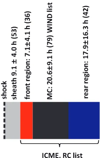
Fig. 1. This figure shows the shock, sheath and different regions within an ICME. Note that not all ICMEs are fast enough to drive shocks, and thus they do not have a well-defined sheath region ei-ther. The ICME interval is obtained from the Richardson and Cane ICME list, and the MC interval from the Wind magnetic cloud list. The widths are scaled to represent relative average durations of dif-ferent regions for our data set (given in the figure and followed by standard deviations). The numbers in parenthesis represent the num-ber of events used to calculate the average durations.
these catalogs are Lepping et al. (2006) and Richardson and Cane (2010). At the time of this study the WIND list covered the period in 1995–2009 and the RC list the period in 1996– 2011. Our study period is when these lists overlap, i.e., from January 1996 to December 2009.
The Wind list includes only MCs. The event and boundary identifications are based primarily on the plasma and mag-netic field parameters. The boundary times are refined based on the results of the fitting the magnetic field data using a force-free, cylindrically symmetric flux-rope model by Lep-ping et al. (1990). However, not all events in the Wind list fulfill the original MC definition by Burlaga et al. (1981) (see Sect. 1), but it has become customary to use the term “mag-netic cloud” to refer to an ICME that contains a mag“mag-netic flux rope (e.g., see discussion in Rouillard, 2011).
primarily from magnetic field and plasma data and assigned to the nearest hour. In the cases where ICME boundaries de-termined from the plasma and field data do not coincide with compositional/charge state signatures, the offsets are indi-cated. We use here boundary times determined from plasma and magnetic field data.
We call the region between the ICME and MC front boundaries as the “MC front region” and the region between the MC and ICME tail boundaries as the “MC rear region” (see Fig. 1). We separate these three regions because they may be generated by fundamentally different processes, ei-ther at the Sun or while the ICME propagates through the interplanetary medium. We emphasize that the front region is different from the ICME sheath region, which consists of compressed and heated plasma between the shock and the ICME leading edge. We define that the ICME and MC boundaries “agree” when the boundaries coincide within two hours, and for “significant” difference we require that ICME signatures have to extend for at least six hours past the MC boundaries. In Fig. 1 we have scaled the widths to repre-sent relative durations of different regions for our data set. The durations of the front and rear regions are calculated for the subsets with ICME and MC boundaries differing by at least two hours. An interplanetary shock was identified for 53 ICMEs from the total of 79 events included in our final data set (see Sect. 3.1). The sheath duration is calculated for this subset.
We shortly summarize below the most common ICME sig-natures (Gosling, 1990; Neugebauer and Goldstein, 1997; Richardson and Cane, 2004a; Zurbuchen and Richardson, 2006): the magnetic field in an ICME is typically enhanced with respect to the ambient value and has low variance. The field directional changes are often coherent, and in the case of an MC a smooth rotation in the field components lasts about one day. However, there are ICMEs whose magnetic field is variable both in magnitude and direction (e.g., see Fig. 4 in Richardson and Cane, 2010). One of the most widely used ICME signatures is the low proton temperature, presumably related to the expansion of the CME when it moves away from the Sun. The measured proton temperatures in ICMEs are typically lower than “the expected proton temperature” (Tex) based on the solar wind speed–proton temperature de-pendence derived by Richardson and Cane (1995). An on-going expansion is revealed by declining bulk speed profile within the ICME, although the interaction with the ambient solar wind may lead to flat or increasing speed profiles. A combination of high magnetic field and depressed temper-ature leads to low values of proton beta. Suprathermal so-lar wind electrons with energies above∼80 eV can be used to diagnose the magnetic connection to the Sun. A coun-terstreaming signature in suprathermal pitch angle spectro-grams during ICMEs is interpreted to present a magnetically closed structure attached to the Sun at both ends. ICMEs also exhibit various compositional and charge state anoma-lies (e.g., Zwickl et al., 1983; Lepri et al., 2001; Richardson
and Cane, 2004a), the most commonly observed being the enhanced helium to proton ratio (He/p), enhanced O+7/O+6 ratio and high mean charge state of iron (< QFe>). As dis-cussed in Sect. 1 all the above mentioned signatures are rarely present in a given ICME and different signatures do not necessarily coincide temporally.
2.3 Analysis parameters
In the analysis we use three output parameters from the Lep-ping et al. (1990) flux rope fitting procedure, which are found in the Wind list. The parameters are quality of the fit (Q0), inclination of the MC axis with respect to the ecliptic plane (θMC), and the relative closest approach distance (|CA|) from the MC center.Q0measures the flux rope model’s ability to fit the magnetic field data for a given event and how it sat-isfies various consistency constraints.Q0can take values of 1, 2 and 3, with 1 meaning a good and 3 a poor fit. For cri-teria to estimateQ0see a detailed description in Lepping et al. (2006).|CA|is calculated as the ratio of the closest ap-proach distance from the MC center to the model estimate of the MC radius.|CA| =0 % means that the MC is crossed centrally and the distance from the center increases as|CA| increases.|CA| =100 % thus means an encounter through the edge of the MC, but there are a few cases in our data set withCA >100 %. As explained by Lepping and Wu (2010) this is due to the uncertainty in|CA|, the actual value of|CA| for such events is usually very near 100 %.
In addition to|CA|we have used the estimates of the im-pact parameter given in the UCLA (University of California, Los Angeles) ICME catalog (UCLA list, 2009) maintained at the ACE Science Center. Defining the total pressure per-pendicular to the magnetic field,Pt, by the sum of the total magnetic pressure and plasma kinetic pressure perpendicular to the magnetic field, the ICMEs can be classified into three groups (Jian et al., 2006): in Group 1 thePtprofile has a cen-tral maximum, in Group 2 it has a plateau-like profile and in Group 3 a gradual decrease is observed after a sharp increase at the leading edge. The Group 1 ICMEs are crossed close to the center of the flux rope, while for Group 2 and Group 3 the impact parameter from the center increases.
2.4 Example event
Figure 2 illustrates an ICME observed on 20–21 May 2005. The pair of red lines bounds the ICME interval (as indicated in the RC list) and the dashed black lines the MC interval (as indicated in the Wind list). At the ICME leading edge the magnetic field magnitude increases and the field becomes less variable, and the He/p and O+7/O+6ratios as well as
a)
b)
c)
d)
e)
f)
g)
h)
i)
j)
k)
2005 5/19 5/20 5/21 5/22 5/23
Fig. 2. ACE observations of an event observed on 20–21 May 2005. The panels show from top to bottom: (a)–(c) magnetic field mag-nitude, latitude and longitude angles in GSE, respectively, (d) solar wind speed, (e) density, (f) measured proton temperature (red line) and expected proton temperature (blue line), (g) perpendicular to-tal pressure, (h) plasma beta, (i) suprathermal electron pitch angle spectrogram at 272 eV, (j) helium to proton ratio (red), O+7/O+6 ratio (purple), and (k) mean iron charge state. The red solid lines bound the ICME interval (from the RC list) and the pair of black dashed lines the MC interval (from the Wind list). The highlighted region marks the interval of the unperturbed flux rope from the Grad–Shafranov reconstruction; for details of which see Sect. 4.
proton temperature, charge state and compositional anoma-lies, continue 19 h past the MC trailing edge. However, it is seen that He/p, O+7/O+6, and< QFe>are lower and tem-perature slightly higher in the rear region than in the MC. In addition, the magnetic field magnitude decreases consid-erably and field variability increases in the rear region. The suprathermal electron spectrogram given in Fig. 1i shows pri-marily unidirectional flow during most of the ICME.
In total, the ICME interval exceeds the MC interval by al-most a day (22.8 h) and the estimated radial widths (duration multiplied by the average speed) are 0.49 AU and 0.26 AU for the ICME and MC, respectively.
According to the UCLA list this ICME was centrally crossed (Group 1), which is evident from thePtprofile show-ing a clear central maximum (Fig. 2g). The Leppshow-ing et al. (1990) flux rope fitting yielded a high-inclination MC axis,
Dt (hours)LE
Dt (hours)TE
[image:5.595.309.545.58.374.2]SSN
Fig. 3. Differences in ICME and MC leading edge times (top panel) and trailing edge times (middle panel). The bottom panel shows the (black) monthly and (red) monthly smoothed sunspot numbers from the Solar Influences Data Center. In the two top panels we have subtracted ICME leading and trailing edge times from the MC leading and trailing edge times. Horizontal lines show±2 and±6 h that we have used as thresholds to mark the cases where boundary times agree or differ significantly. The different symbols indicate the spacecraft’s closest approach distance (given in the UCLA list) from the MC center as estimated from the perpendicular pressure profile (green circle: central cut, light-blue star: ICME crossed from the intermediate distances from the center, purple X: ICME flanks encountered, black triangle:Ptcategory could not be determined).
(θMC=59◦), and|CA| =34 %, indicating the encounter at the intermediate distance from the MC center. The quality of the fitting is satisfactory (Q0=2).
3 Statistical results
3.1 Relationship between the MC and ICME bound-aries
In total, we found 82 events that were included both in the RC list and in the Wind list. Figure 3 displays calcu-lated differences in the ICME and MC leading edge times (1tLE=tLE,ICME−tLE,MC) and trailing edge times (1tTE=
[image:5.595.50.287.60.360.2]1tLE mean that the ICME leading edge was before (after) the MC leading edge and the positive (negative) values of
1tTEthat the ICME trailing edge was before (after) the MC trailing edge. Note that they axis scale in the two top pan-els of Fig. 3 is the same to highlight that the boundary time differences are much larger at the trailing edge than at the leading edge.
There was one event for which the MC front boundary started more than six hours before the ICME front boundary and two events for which the MC rear boundary extended by more than six hours beyond the ICME boundaries. We have excluded these periods from the analysis because they are inconsistent with the definition that an MC is a substruc-ture of the ICME (e.g., see discussion by Richardson and Cane, 2010). As discussed earlier the definitions of ICMEs and MCs are not unambiguous, which may lead to incorrect boundary identifications.
The ICME and MC leading boundaries coincided within two hours in 54 % (43/79) of the studied cases and the trail-ing boundaries in 46 % (36/79) of the studied cases. Only in 30 % (24/79) of the cases the boundaries coincided both at the front and the rear edge. The ICME leading edge pre-ceded the MC leading edge by more than six hours in 22 % (17/79) of the studied cases. For the subset with1tLE<−6 h the mean time difference between the ICME and MC bound-aries was 10.2 h with a standard deviation of 2.8 h. In turn, in 38 % (30/79) of the cases the ICME trailing edge occurred more than six hours after the MC trailing edge and the mean difference was 22.7 h with a standard deviation of 16.9 h.
As a consequence of the frequent mismatch between the MC and ICME boundaries, it can make a large difference whether it is the ICME interval or the MC interval that is used to calculate the event characteristics, such as the mean speed, duration and average width. In 39 % (31/79) of the events the duration of the ICME exceeds the duration of the MC by more than 12 h. The differences in mean speeds and magnetic fields were not so significant, only in five events the differences were larger than 50 km s−1or 5 nT. The large variations in durations lead also to significant differences in radial widths (duration multiplied by the average speed), in 44 % of the studied cases the radial width of the ICME ex-ceeded the MC width by at least 0.1 AU.
[image:6.595.330.519.63.222.2]As the fraction of MCs from ICMEs varies depending on the solar activity cycle, we also investigate whether there is a solar cycle dependence in the location of ICME and MC boundaries. From Fig. 3 we see that the differences in bound-ary times are larger during high solar activity than near solar minimum. In total, our statistics include 30 events near or during solar minimum (1996–1997 and 2006–2009). In 48 % of these cases the ICME and MC boundaries coincided and in 26 % there was a significant mismatch (either at the front or rear edge or at both edges). During the years of higher solar activity (1998–2005) there were 49 events. The ICME and MC boundaries coincided only in 16 % of the cases and
|CA| (%) a)
b)
back region duration (hours) front region duration (hours)
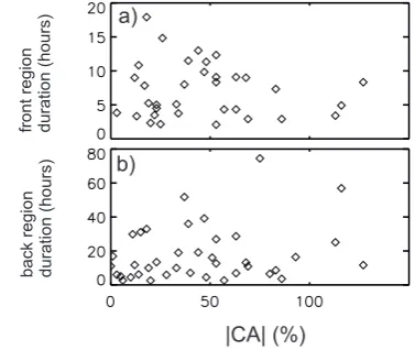
Fig. 4. Top: Duration of the MC (a) front and (b) rear regions as a function of the relative closest approach distance|CA|(from the Wind list).
differed significantly in 61 % of the cases. We discuss this in more detail in Sect. 5.
3.2 Relation of the impact parameter to ICME and MC boundaries
DifferentPtcategories are indicated in Fig. 3 (see figure cap-tion and Sect. 2 for definicap-tions). In Table 1 we give the num-ber of events in eachPtgroup for cases where the boundaries either agreed or differed significantly at the front and rear edges. From those 75 events for which thePt group could be assigned 59 % (44/75) were crossed centrally (Group 1), 28 % (21/75) at intermediate distances from the MC center (Group 2) and only 13 % (10/75) of events were intercepted on the flanks (Group 3). Centrally crossed MCs formed a clear majority in each case considered, although their frac-tion was smallest (40 %) for the subset with1tTE>6 h. In addition, the fraction of events in Group 3 was smaller for the events with coinciding boundary times than for the events with1tLE<−6 h and1tTE>6 h.
Figure 4 shows that there is no correlation of the dura-tions of the MC front and rear regions with the relative clos-est approach distance from the MC center (|CA|). However, the cases where MC and ICME boundaries coincided had on average somewhat smaller |CA| values than the cases where they differed considerably. The average|CA| values were 32.9 and 42.2 % for the subsets with|1tLE|<2 h and
1tLE<−6 h, respectively, and 31.1 and 41.9 % for the sub-sets with|1tTE|<2 h and1tTE>6 h, respectively.
Table 1. The row “All” shows the distribution of all studied events to differentPtgroups and the flux rope fitting quality (Q0) categories
(see Sect. 2 for definitions). Note that thePtgroup could be assigned only for 75 of events, while the quality category was available for all 79 events in our data set. The following rows show distributions separately for the events where the ICME and MC boundaries agreed (|1tLE|<2 h and|1tTE|<2 h) and for the events where the boundaries differed significantly (1tLE<−6 h and1tTE>6 h). The second
column gives the total number of events in these categories (used to compute all percentages).
Events Group 1 Group 2 Group 3 QO=1 QO=2 QO=3
All 75/79 44 (59 %) 21 (28 %) 10 (13 %) 14 (18 %) 35 (44 %) 30 (38 %)
|1tLE|<2 h 40/43 24 (56 %) 12 (28 %) 4 (9 %) 6 (14 %) 23 (53 %) 14 (33 %) 1tLE<−6 h 16/17 9 (53 %) 4 (24 %) 3 (18 %) 4 (24 %) 7 (41 %) 6 (35 %) |1tTE|<2 h 34/36 24 (67 %) 8 (22 %) 2 (6 %) 8 (22 %) 13 (36 %) 15 (42 %) 1tTE>6 h 27/30 12 (40 %) 10 (33 %) 5 (17 %) 4 (13 %) 14 (47 %) 12 (40 %)
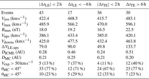
Table 2. Comparison of the ICME characteristics between the events where the ICME and MC boundaries agreed (|1tLE|<2 h and|1tTE|<
2 h) and where the boundaries differed significantly (1tLE<−6 h and1tTE>6 h). The rows give from top to bottom the averages of the
ICME average speed (Vave), maximum speed (Vmax), maximum magnetic field magnitude (Bmax), 12 h averaged upstream (Vups) and downstream (Vdowns) speeds, the speed difference (when positive) between the ICME leading edge speed andVup (1VLE,ups), the ICME
radial width (DICME), and the MC radial width (DMC). The panelVexp>50 km s−1gives the number of events in each category when the
expansion speed of the ICME exceeded 50 km s−1. The two bottom rows give the distribution of events to low-inclination (θMC<45◦) and
high-inclination (θMC>45◦) MCs.
|1tLE|<2 h 1tLE<−6 h |1tTE|<2 h 1tTE>6 h
Events 43 17 36 30
Vave(km s−1) 422.4 468.5 415.7 483.1
Vmax(km s−1) 485.9 566.2 470.0 596.1
Bmax(nT) 18.0 19.2 16.5 22.5
Vups(km s−1) 386.1 433.4 385.0 420.1
Vdowns(km s−1) 425.0 477.5 432.4 463.8
1VLE,ups 79.0 90.0 49.8 133.7
DICME(AU) 0.28 0.46 0.24 0.51
DMC(AU) 0.21 0.25 0.21 0.20
Vexp>50 km s−1 5 (13 %) 7 (37 %) 4 (11 %) 12 (40 %)
θMC<45◦ 33 (77 %) 12 (71 %) 24 (67 %) 23 (77 %) θMC>45◦ 10 (23 %) 5 (29 %) 12 (33 %) 7 (23 %)
of ten events where MC and ICME boundaries differed sig-nificantly both at the leading and trailing edges, three were in Group 1 and two had|CA|<33 %.
3.3 Relation of flux rope fitting quality to ICME and MC boundaries
In Table 1 we also show the division of the events to different quality groups given in the Wind list (see Sect. 2). Only 18 % of the studied events haveQ0category 1 i.e., a good fit. There is no clear trend that the extended MC rear and front regions could be explained by poor quality (Q0=3) of the MC fit-ting. The distributions of the studied events to differentQ0 categories are rather similar for the cases where the MC and ICME boundaries agree and where they differ significantly.
3.4 General differences in event characteristics
We investigate next whether there are differences in charac-teristics between events where ICME and MC boundaries agree and where they differ significantly. The results are gathered in Table 2 and except for the MC width, the values were calculated using the ICME interval. The average solar wind speed upstream and downstream of the ICME were cal-culated as 12 h averages. For the ICMEs that drove a forward shock, the upstream values were calculated using the 12 h in-terval before the shock. We have considered separately the cases where differences occurred at the leading edge and at the trailing edge.1VLE,upsgives the difference between the ICME leading edge speed and the upstream solar wind speed.
[image:7.595.148.450.321.481.2]Table 2 shows that the ICMEs with significant differences, either at the front edge or at the trailing edge, are on av-erage stronger and faster. The tendency to have high mag-netic fields is particularly clear in the subset with1tTE>6 h; the mean maximum magnetic fields for the subsets with |1tTE|<2 h and 1tTE>6 h were 16.5 and 22.5 nT. In ad-dition, the ICMEs with 1tTE>6 were clearly faster than the preceding solar wind; the average values of 1VLE,ups were 49.8 and 133.7 km s−1for the subsets with|1tTE|<2 h and1tTE>6 h, respectively. The corresponding values were 79.0 and 90.0 km s−1 for the events with |1tLE|<2 h and
1tLE<−6 h, respectively. The events with significant mis-match in boundary times experienced also stronger expan-sion at 1 AU and were embedded in a faster solar wind than the events for which the boundary times coincided. The ICME width (DICME) was considerably larger when bound-aries disagreed than when they coincided, but interestingly, the width of the MC was very similar for all cases consid-ered.
We also checked whether the inclination (θMC) of the MC axis affects the relative locations of the ICME and MC boundaries. The last two rows of Table 2 show the distri-bution of the studied events to low- (θMC<45◦) and high-inclination (θMC>45◦) MCs. The events with1tLE<−6 h had similar distribution to low- and high-inclination MCs as the cases for which the front boundary times agreed, while the events with1tTE>6 h have a slight tendency to be low inclined more often than the events for which the end bound-ary times agreed.
3.5 Characteristics of MC and non-MC parts
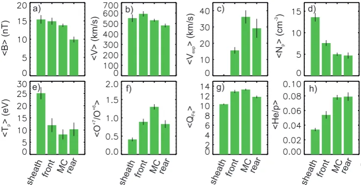
We have calculated the average values of selected solar wind parameters in the sheath, in the MC and in the MC front and rear regions (Fig. 5). We see that the sheath has clearly the most compressed plasma (the highest average density and temperature) and also the highest magnetic field magnitude. Within the ICME, the front region has the highest density, temperature and magnetic field magnitude. The temperature is lowest within the MC, while the rear region has consid-erably lower magnetic field magnitude than the other inves-tigated regions. The solar wind speed is highest in the front region and lowest in the rear region, but no large variations are observed. It is seen that the MC experiences the strongest expansion and that the significant expansion continues also in the rear region. However, the front region has a considerably smaller average expansion speed. All except one investigated sheath region had a positive speed gradient, and thus we do not give the average expansion speed value for the sheath in Fig. 5c. Finally, Fig. 5f–h show that the O+7/O+6 ratio and the mean iron charge states had highest values within the MC, while the He/p ratio was most enhanced in the MC and rear region. The sheath stands out as the region with the lowest charge state values and the lowest He/p ratio.
It has been suggested that radial magnetic field intervals observed occasionally after MCs would signal the spacecraft encountering the leg of the ICME. We consider the field to be nearly radial when the ratio of the magnetic fieldX com-ponent (BX) to the magnetic field magnitudeB was larger than 0.7 (Neugebauer and Goldstein, 1997). We calculated the percentage ofBX/B >0.7 in the MC rear region for each event with1tTE>6 h. Five out of 30 events (17 %) had a radial magnetic field for more than one-third of the rear re-gion duration. The fractions of radial magnetic fields in these events ranged from 38 to 60 % or 26.9 to 74.5 h.
4 Example events
In this section we perform a detailed analysis of two events that show significant differences in ICME and MC bound-ary times. We use Grad–Shafranov (GS) reconstruction (Hu and Sonnerup, 2002; M¨ostl et al., 2008; Isavnin et al., 2011) to investigate the structure of the flux ropes in these events. In addition, we find the associated CMEs from white-light LASCO coronagraph observations.
GS reconstruction uses in situ measurements of magnetic field and plasma parameters as input and produces the di-rection of the invariant axis of the flux rope and the recon-struction of the local cross section of the flux rope as output. The flux rope is assumed to have 2.5-dimensional structure, i.e., the magnetic field is assumed to have translation sym-metry with respect to an invariant axis direction. The 2.5-dimensional magnetic structures with the invariant axis along
zaxis can be described with the GS equation:
∂2A ∂x2 +
∂2A ∂y2 = −µ0
d dA p+
Bz2
2µ0 !
, (1)
where A is the magnetic vector potential, such that A=A(x, y)zˆ, and the magnetic field vector is B= [∂A/∂y,−∂A/∂x, Bz(A)]. The plasma pressure, the pres-sure of the axial magnetic field component and thus their sumPt=p+Bz2/2µ0(transverse pressure) are functions of
Aalone. The GS reconstruction is performed by numerically solving Eq. (1). The crucial point in the reconstruction tech-nique is the determination of the flux rope invariant axis di-rection, which is based on the assumption of constant mag-netic vector potential and transverse pressure on common magnetic field lines. Pt(A) curve consists of two branches corresponding to the parts of the spacecraft trajectory mov-ing inward and outward of the flux rope. For the optimal di-rection of the invariant axis two branches coincide.
a) b) c) d)
e) f) g) h)
<B> (nT) <V> (km/s)
<V > (km/s) exp <N > (cm ) p -3 <T
> (eV)p
<O /O > +7 +6 <Q > Fe <He/p> sheath front MC rear sheath front MC rear sheath front MC rear sheath front MC rear
Fig. 5. Comparison of selected solar wind parameters in sheath, front region, MC, and rear region. The panels give the averages of a) magnetic field, b) average solar wind speed, c) expansion speed, d) density, e) temperature, a) O+7/O+6, b) mean iron charge state, and c)
He/p. The standard error of the mean is given in each histogram.
In addition, we find the associated CMEs from white-light 555
LASCO coronagraph observations.
GS reconstruction uses in-situ measurements of magnetic field and plasma parameters as input and produces the direc-tion of the invariant axis of the flux rope and the reconstruc-tion of the local cross-secreconstruc-tion of the flux rope as output. The 560
flux rope is assumed to have 2.5-dimensional structure, i.e. the magnetic field is assumed to have translation symmetry with respect to an invariant axis direction. 2.5-dimensional magnetic structures with the invariant axis alongzaxis can be described with the GS equation:
565
∂2A
∂x2 +
∂2A
∂y2 =−µ0 d dA
p+B
2
z
2µ0
, (1)
where A is the magnetic vector potential, such that
A =A(x,y)ˆz, and the magnetic field vector is B= [∂A/∂y,−∂A/∂x,Bz(A)]. The plasma pressure, the pres-sure of the axial magnetic field component and thus their 570
sumPt=p+Bz2/2µ0(transverse pressure) are functions of
Aalone. The GS reconstruction is performed by numerically solving Equation 1. The crucial point in the reconstruction technique is the determination of the flux rope invariant axis direction which is based on the assumption of constant mag-575
netic vector potential and transverse pressure on common magnetic field lines. Pt(A)curve consists of two branches corresponding to the parts of the spacecraft trajectory mov-ing inward and outward of the flux rope. For the optimal direction of the invariant axis two branches coincide. 580
The boundary of the flux rope is defined as the absolute minimum of the magnetic potential for which two branches ofPt(A)still coincide. GS reconstruction has been shown to be able to deduce the boundaries of the non-perturbed flux-rope within an ICME (Isavnin et al., 2011). We use this
property of GS reconstruction as an aid in comparison of the ICME boundaries for these events listed in RC and Wind cat-alogues and analysis of the reasons behind their significant difference.
4.1 May 20–22, 2005
590
As discussed in Section 2 (see Figure 2) in the May 20–22, 2005 event the ICME-related signatures began a few hours before the MC leading edge and continued 19 hours beyond the MC trailing edge.
According to the GS reconstruction, the unperturbed flux 595
rope was observed on May 20, 1430 UT – May 21, 0330 UT (highlighted in Figure 1), i.e. the passage of the GS flux rope started 8.5 hours later than the MC and ended 1.5 hours ear-lier than the MC. The detailed visual inspection of Figure 2 also reveals that the GS flux rope confined the highest mag-600
netic fields and smoothest field rotation, as well as declin-ing portion in speed and clearest compositional/charge state anomalies.
The front boundary of the GS flux rope was separated from the preceding plasma by a clear substructure (May 20, 1450 605
- 1510 UT) featuring a decrease in the magnetic field magni-tude and enhancements in proton density, temperature, beta and speed. A broader and weaker substructure was also detected at the MC/flux rope rear edge between May 21, 0510 -0936 UT, showing enhanced density, slightly increased tem-610
perature and plasma beta as well decreased magnetic field. The inclination of the flux rope axis depends on the chosen boundary interval. As mentioned in Section 2, for the MC interval calculated in the Wind list, the Lepping, Jones and Burlaga (1990) force-free fitting gave highly inclined axis
Fig. 5. Comparison of selected solar wind parameters in sheath, front region, MC, and rear region. The panels give the averages of (a) mag-netic field, (b) average solar wind speed, (c) expansion speed, (d) density, (e) temperature, (a) O+7/O+6, (b) mean iron charge state, and (c) He/p. The standard error of the mean is given in each histogram.
ICME boundaries for these events listed in the RC and Wind catalogues and analysis of the reasons behind their signifi-cant difference.
4.1 20–22 May 2005
As discussed in Sect. 2 (see Fig. 2) in the 20–22 May 2005 event the ICME-related signatures began a few hours before the MC leading edge and continued 19 h beyond the MC trailing edge.
According to the GS reconstruction, the unperturbed flux rope was observed on 20 May, 14:30 UT–21 May, 03:30 UT (Universal Time; highlighted in Fig. 1), i.e., the passage of the GS flux rope started 8.5 h later than the MC and ended 1.5 h earlier than the MC. The detailed visual inspection of Fig. 2 also reveals that the GS flux rope confined the high-est magnetic fields and smoothhigh-est field rotation, as well as declining portion in speed and clearest compositional/charge state anomalies.
The front boundary of the GS flux rope was separated from the preceding plasma by a clear substructure (20 May, 14:50– 15:10 UT) featuring a decrease in the magnetic field magni-tude and enhancements in proton density, temperature, beta and speed. A broader and weaker substructure was also de-tected at the MC/flux rope rear edge between 21 May, 05:10– 09:36 UT, showing enhanced density, slightly increased tem-perature and plasma beta as well decreased magnetic field.
The inclination of the flux rope axis depends on the chosen boundary interval. As mentioned in Sect. 2, for the MC in-terval calculated in the Wind list, the Lepping et al. (1990) force-free fitting gave highly inclined axis (inclination of 59◦), while the GS flux rope lies closer to the ecliptic plane, with inclination of 38◦.
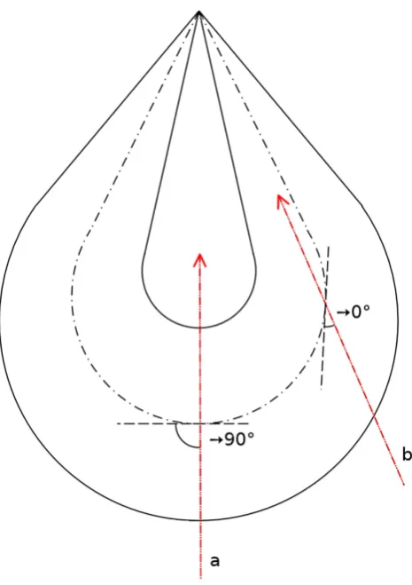
The geometry of the spacecraft trajectory through the flux rope can be estimated using the following simple logic: as-suming that the flux rope loop is not severely deformed at 1 AU, the angle between the local orientation of the invariant axis of the flux rope and the Sun–spacecraft line is close to 90◦if the spacecraft crossed the loop near the apex. On the other hand, if the spacecraft crossed the loop through or near the leg of the flux rope, the defined angle tends to 0◦ (see Fig. 6). The angle between the local direction of the invari-ant axis of the flux rope and the Sun–spacecraft line is 59◦for
this event, which means that the trajectory of the spacecraft went relatively close to the apex of the flux rope loop.
There are two partial halo CMEs in the LASCO CME catalogue that we have considered as the source of the 20– 21 May ICME. The first CME was observed in LASCO/C2 on 16 May, 14:50 UT and the second on 17 May, 03:26 UT. The plane-of-the-sky speed (from the LASCO catalogue) for these CMEs were 256 and 449 km s−1, respectively and the angular widths 140◦and>273◦, respectively.
[image:9.595.113.482.62.251.2]Fig. 6. Schematic representation of the spacecraft trajectory through the flux rope (the global flux rope structure is an adaptation from Burlaga et al., 1990). Trajectory a corresponds to the crossing close to the apex of the flux rope loop. Trajectory b is the crossing through the leg of the flux rope loop. The angle between the local orientation of the invariant axis of the flux rope and the Sun–spacecraft line goes from 90◦for the case a to nearly 0◦for the case b.
The 16 May CME shows a clear flux rope structure in coronagraph images (“loop-type” according to classification in Vourlidas et al., 2012), but its axis was elongated SE–NW, and thus it seems unlikely that the Earth would have inter-cepted this CME through the apex. The flux rope structure for the 17 May CME is not evident from coronagraph im-ages, but its axis lied along the north–south line suggesting the high-inclination flux rope. The 17 May CME was also as-sociated with a clear EIT (Extreme ultraviolet Imaging Tele-scope) dimming between 02:48–05:10 UT near AR 10763 and there was continuing activity from this active region after the CME, including some small ejections.
Based on the considerations above it is difficult to judge which of the CMEs reached Earth. The central location of the 17 May CME, clear EIT dimming and continuing activ-ity from the source AR makes it a candidate for producing an MC with an extended rear region that was crossed close to the center by the spacecraft located along the Sun–Earth
a)
b)
c)
d)
e)
f)
g)
h)
i)
j)
k)
2001 4/28 4/29 4/30 5/1 5/2
Fig. 7. Example of the event on 28 April–1 May 2001. Panels are same as in Fig. 2. The pair of red lines bound the ICME interval and the pair of black, dashed lines the MC interval. The dash-dotted line indicates the interplanetary shock, and the highlighted region the interval of the unperturbed flux rope from the Grad–Shafranov reconstruction.
line. In addition, the north–south oriented CME axis matches the highly-inclined MC. It is possible that the GS flux rope presents the unperturbed part of a highly inclined larger flux rope (approximately the Wind MC). As both CMEs were slow and originated from different ARs it does not seem plau-sible that the 17 May CME would have merged into the ear-lier CME, but it is possible that it interacted with the flank of the 16 May CME while leaving the Sun.
4.2 28 April 2001
Magnetic field and plasma measurements for the second ex-ample that took place on 28 April 2001 are shown in Fig. 7. This event had significantly extended MC front and rear re-gions. The ICME drove a strong forward shock that was ob-served at ACE on 28 April at 04:32 UT. The following sheath region was featured by rapid and large amplitude fluctua-tions in the magnetic field direction, high temperature and plasma beta. At the ICME leading edge the magnetic field became smoother, temperature decreased significantly below
[image:10.595.310.545.61.362.2]MC, the magnetic field rotation was clear and the speed de-clined strongly.
In the MC rear region the magnetic field magnitude de-creased close to the typical quiet solar wind value (∼5 nT), but several ICME-related signatures continued; the solar wind speed declined monotonically, temperature was de-pressed belowTex, field variance was relatively low and the He/p and O+7/O+6 ratios and the iron charge states were strongly enhanced. In fact, the highest He/p and O+7/O+6 values occurred in the rear region.
This example event also highlights the difficulties in deter-mining the ICME boundaries. According to the RC list (and seen from Fig. 7i and j) the abnormal compositional/charge state signatures continued more than a day beyond the ICME trailing edge and plasma beta was relatively low. The main feature of the marked ICME trailing edge is the proton tem-perature increasing to match approximatelyTex.
The direction of the magnetic field remained rather sta-ble in the rear region and the magnetic field profile was rel-atively smooth and did not feature any strong fluctuations. The suprathermal electron spectrogram shows a strong de-pletion concentrated at PA=90◦ that continued from the ICME leading edge long after its trailing edge together with compositional/charge anomalies. The strongest heat flux was obviously observed at PA=0◦, but there was also a weak flow antiparallel to the magnetic field direction.
This event is Group 2 in the UCLA list, thus suggesting the crossing from the intermediate distance from the flux rope center. According to analyses performed in the Wind list the MC had low inclination,θMC=12◦, and|CA| =39 %, also indicating the encounter at the intermediate distance from the MC center. The quality of the flux rope fitting was satisfac-tory (Q0=2).
As seen in Fig. 7, for this event the GS flux rope coincided approximately with the MC. Close to the front boundary of the MC/GS-flux rope on 29 April, 00:00–00:35 UT, a sub-structure similar to the one detected at the front boundary of the 20–22 May 2005 GS-flux rope (Sect. 4.1) was observed. In turn, the transition from the MC/GS flux rope to the MC back region was relatively smooth.
The local orientation of the invariant axis differs by 24◦ from the Sun–spacecraft line. According to our analysis this event is similar to casebdepicted in Fig. 6, i.e., the spacecraft encountered the flux rope through one of its legs. Figure 7k shows that strong pitch angle depletion and weak counter-streaming were observed also in the MC rear region and the magnetic field remained as smooth as inside the MC al-though no rotation was detected. These two facts strongly support our leg encounter hypothesis. While moving through the leg of the flux rope the spacecraft trajectory remained approximately parallel to the invariant axis of the flux rope. Hence, the magnetic field remained smooth, but no rotation was measured. In addition, this was also one of the few events that showed significant amount of radial magnetic field in the rear region (see Sect. 3.5). The region of radial magnetic field
began just after the MC trailing edge and continued 36 h, cov-ering 38 % of the rear region. In conclusion, the reason why ICME and MC/flux rope boundaries did not coincide for this event seems to be geometrical.
The candidate CME appeared on 26 April at 12:30 UT in the LASCO/C2 field of view. According to the LASCO cata-logue the plane-of-the-sky speed was 1006 km s−1 and the estimated arrival time to 1 AU using this speed as the in-put to the Gopalswamy et al. (2001) model is on 29 April at 00:45 UT. This time matches very well with the MC/GS-flux rope leading edge time on 29 April at 02:00 UT. There were no other possible wide CME candidates within a suit-able time window.
The CME originated in the northeast corner of AR 09433, which extended from N23W2 to N16W16. Coronagraph im-ages revealed a clear flux rope structure (loop-type) and a shock could be discerned from the white-light data along the NE extent of the CME. The CME was associated with a C6.8 flare. The observations show a rather circular CME with axis oriented NE–SW, thus being also in accordance with the Earth intercepting the leg of the CME.
5 Summary and discussion
The motivation for our study stemmed from the long-standing issue of whether all CMEs are intrinsically flux ropes and why only a relatively small fraction of ICMEs in situ show flux rope (or in other words MC) signatures. We tackled this problem by examining cases where ICME and MC boundaries coincided and when they differed signif-icantly. We summarize our main findings as follows.
– The significant difference (>6 h) between ICME and MC boundaries occurred more often at the trailing boundary (38 % of 79 studied cases) than at the leading boundary (22 %) and the mean difference was larger.
– Events for which the ICME signatures continued
signif-icantly past the MC rear boundary had 2.7 times larger speed difference with respect to the preceding solar wind, had 1.4 times stronger peak magnetic fields, were 2.1 times larger and were three times more likely to ex-perience significant expansion than the events for which the rear boundaries coincided. Similar trends, although with weaker differences, were found for the events with significant mismatch in the front boundary times.
– ICME/MC boundary time differences are not generally
due to a geometrical effect (large impact parameter or encounter through the leg).
– The sheath region, MC, and the front and rear
Different properties between the sheath, and MC and non-MC parts in ICMEs suggest that they originate from physi-cally different regions near the Sun. In particular, the charge state composition is determined within a few solar radii from the Sun, and does not change after that. The highest values of O+7/O+6ratio and the mean iron charge states found in MCs indicate that they had the highest temperatures in the low corona (with oxygen freezing in at around 2RSand iron around 5RS). The anomalous charge state signatures, in par-ticular He/p, continuing beyond MC/ICME boundaries was detected already by Richardson and Cane (2004a). A possi-ble explanation for the enhanced He/p towards the rear of the MCs is the result of gravitational settling of helium in the solar corona (Neugebauer and Goldstein, 1997).
Our finding that events with coinciding ICME/MC bound-aries occur during solar minimum while events with signif-icant boundary mismatch occur predominantly during solar maximum and are strong and fast, could be due to two ef-fects: (1) during solar maximum, CMEs occur with increased frequency thus leading to increased chances of CME–CME interaction and disturbed ambient conditions during their he-liospheric propagation. Such interactions will tend to the dis-tort in situ signatures and the event boundaries. (2) CMEs tend to be both more impulsive and to originate from active regions with complex magnetic topologies during solar max-imum. It is therefore likely that the corresponding ICMEs will exhibit more distorted fields and plasma at their front part and also at the trailing part due to enhanced reconnection outflows. In contrast, solar minimum CMEs are predomi-nantly associated with streamer blow-outs and filaments with well-structured morphologies, minimum heating and gradual acceleration profiles (e.g., Sheeley et al., 1999; Vourlidas et al., 2002). We believe that both of these effects contribute to the observed complexity of MC/ICME boundary timing.
As mentioned in Sect. 1 magnetic reconnection at the front of the MC can erode the original flux rope and lead to an ex-tended rear region with low magnetic fields (e.g., see Fig. 1 in Dasso et al., 2007). However, erosion does not explain extended front regions, and furthermore, we found that the MCs had similar widths regardless whether the ICME and MC boundaries coincided or not. If an MC gradually erodes due to magnetic reconnection one would assume that such MCs have smaller radial sizes than non-eroded MCs. This suggests that the solar wind interacts quite strongly with the ICME, but the MC is quite oblivious to its surroundings. As shown by Vourlidas et al. (2000) the flux rope core of the CME is an isolated system based on the evolution of their energies. However, one should remember that the majority of events where boundary times agreed occurred near solar minimum when MCs and ICMEs tend to be smaller than near solar maximum when the majority of events with large differ-ences in boundary times were observed. The detailed study on the role of erosion in forming extended back regions will be left for a future study.
How does then the five-part white-light CME morphology (see Sect. 1) compare with in situ observations? As shown in this work the ICME sheath and front region have in gen-eral different characteristics, and in particular the different charge state values support the view that they have different origin. We suggest that the bright front surrounding the cav-ity in white-light images corresponds to the MC front region. Thus, the front region is formed from coronal loops piled up at the flux rope boundary. In contrast, the sheath region largely forms during the CME’s interplanetary travel and has no clear signature yet in coronagraph images.
The MC/flux rope observed in situ corresponds to the unperturbed part of the white-light cavity. Refined analy-sis methods, such as Grad–Shafranov reconstruction (see Sect. 4) can be used to single out the unperturbed flux rope in the interplanetary medium. The brief substructures we found at the flux rope edges for our two example events (Sect. 4) could be signatures of the processes that separate the flux rope from the surrounding ICME. Such substructures have been reported regularly at MC/flux ropes boundaries (e.g., Farrugia et al., 2001; Wei et al., 2002; Andreeova et al., 2013) and their electron and proton flux variations are similar to those in the reconnection exhausts (Wang et al., 2012).
We suggest that the parts of the initial flux rope ejected from the Sun that are deformed during the interplanetary travel add to the MC front and rear regions. Most of the ex-tended rear region is nevertheless associated to the stretching of magnetic fields by the outward moving CME and contin-uing ejection from the source region as well as possible ero-sion during the interplanetary propagation. Thus, there is no clear correspondence of the rear region either in the white-light CME morphology presented by Vourlidas et al. (2012). It should be noted that in this work, we did not investigate en-hanced density regions in the trailing part of the flux ropes or in the rear regions. Such density “plugs” can be remnants of the bright prominence core. However, as suggested in Vourl-idas et al. (2012) the prominence material mostly falls back to the Sun or is heated to coronal temperatures, and conse-quently its identification in situ is difficult.
As the result of this work we identify five distinct regions in situ related to a CME eruption; shock, sheath, front region, flux rope/MC, and rear region. Thus, the flux rope is only a part of the complex CME eruption process. An extensive comparison of coronagraph and in situ observations (in par-ticular, the charge state/compositional signatures) by bridg-ing the gap usbridg-ing e.g., heliospheric imager observations, is needed to resolve the details of how remote and in situ CME morphologies are connected.
Acknowledgements. We thank N. Ness for the ACE MFI data,
between ESA and NASA. Academy of Finland project 1218152 is thanked for financial support. A. Vourlidas’ work is supported by NASA contract S-136361-Y to the Naval Research Laboratory. Lu-ciano Rodriguez partially contributes to the research for the Euro-pean Union Seventh Framework Programme (FP7/2007-2013) un-der grant agreement number 263252 [COMESEP]. Luciano Ro-driguez acknowledges support from the Belgian Federal Science Policy Office through the ESA-PRODEX program.
Topical Editor M. Temmer thanks C. Farrugia, V. Bothmer, and one anonymous referee for their help in evaluating this paper.
References
ACE List (Richardson and Cane list): http://www.srl.caltech.edu/ ACE/ASC/DATA/level3/icmetable2.htm.
Andreeova, K., Kilpua, E. K. J., Hietala, H., Koskinen, H. E. J., Isavnin, A., and Vainio, R.: Analysis of the substructure within a complex magnetic cloud on 3–4 September 2008, Ann. Geo-phys., 31, 555–562, doi:10.5194/angeo-31-555-2013, 2013. Bothmer, V. and Schwenn, R.: The structure and origin of
mag-netic clouds in the solar wind, Ann. Geophys., 16, 1–24, doi:10.1007/s00585-997-0001-x, 1998.
Brueckner, G. E., Howard, R. A., Koomen, M. J., Korendyke, C. M., Michels, D. J., Moses, J. D., Socker, D. G., Dere, K. P., Lamy, P. L., Llebaria, A., Bout, M. V., Schwenn, R., Simnett, G. M., Bedford, D. K., and Eyles, C. J.: The Large Angle Spectroscopic Coronagraph, Sol. Phys., 162, 357–402, 1995.
Burlaga, L.: Magnetic clouds and force-free fields with constant al-pha, J. Geophys. Res., 93, 7217–7224, 1988.
Burlaga, L., Sittler, E., Mariani, F., and Schwenn, R.: Magnetic loop behind an interplanetary shock: Voyager, Helios and IMP 8 ob-servations, J. Geophys. Res., 86, 6673–6684, 1981.
Burlaga, L. F., Klein, L., Sheeley Jr., N. R., Michels, D. J., Howard, R. A., Koomen, M. J., Schwenn, R., and Rosenbauer, H.: A mag-netic cloud and a coronal mass ejection, Geophys. Res. Lett., 9, 1317–1320, doi:10.1029/GL009i012p01317, 1982.
Burlaga, L. F., Lepping, R. P., and Jones, J. A.: Global configura-tion of a magnetic cloud, in Physics of Magnetic Flux Ropes, Geophys. Monorg., 58, Washington, AGU, 373–377, 1990. Burlaga, L. F., Plunkett, S. P., and St. Cyr, O. C.:
Succes-sive CMEs and complex ejecta, J. Geophys. Res., 107, 1266, doi:10.1029/2001JA000255, 2002.
Cane, H. V., Richardson, I. G., and Wibberenz, G.: Helios 1 and 2 observations of particle decreases, ejecta, and magnetic clouds, J. Geophys Res., 102, 7075–7086, doi:10.1029/97JA00149, 1997. Cremades, H. and Bothmer, V.: On the three-dimensional
configu-ration of coronal mass ejections, Astron. Astrophys., 422, 307– 322, doi:10.1051/0004-6361:20035776, 2004.
Dasso, S., Nakwacki, M. S., Demoulin, P., and Mandrini, C. H.: Progressive transformation of a flux rope to an ICME. Compar-ative analysis using the direct and fitted expansion methods, Sol. Phys., 244, 115–137, doi:10.1007/s11207-007-9034-2, 2007. Eyles, C. J., Simnett, G. M., Cooke, M. P., Jackson, B. V.,
Buffin-gton, A., Hick, P. P., Waltham, N. R., King, J. M., Anderson, P. A., and Holladay, P. E.: The Solar Mass Ejection Imager (Smei), Sol. Phys., 217, 319–347, 2003.
Farrugia, C. J., Vasquez, B., Richardson, I. G., Torbert, R. B., Burlaga, L. F., Biernat, H. K., Muhlbachler, S., Ogilvie, K. W., Lepping, R. P., Scudder, J. D., Berdichevsky, D. E., Semenov,
V. S., Kubyshkin, I. V., Phan, T.-D., and Lin, R. P.: A reconnec-tion layer associated with a magnetic cloud, Adv. Space Res., 28, 759–764, doi:10.1016/S0273-1177(01)00529-4, 2001.
Gloeckler, G., Bedini, P., Bochsler, P., Fisk, L. A., Geiss, J., Ipavich, F. M., Cani, J., Fischer, J., Kallenbach, R., Miller, J., Tums, O., and Winner, R.: Investigation of the Composition of Solar and Interstellar Matter Using Solar Wind and Pickup Ion Measure-ments with SWICS and SWIMS on the ACE Spacecraft, Space Sci. Rev., 86, 495–539, 1998.
Goldstein, H.: On the field configuration in magnetic clouds, in Solar Wind Five, edited by: Neugebauer, M., Geophys. NASA Conf. Publ., 731–733, 1983.
Gopalswamy, N., Lara, A., Yashiro, S., Kaiser, M. L., and Howard, R. A., Predicting the 1-AU arrival times of coro-nal mass ejecitons, J. Geophys. Res., 106, 29207–29217, doi:10.1029/2001JA000177, 2001.
Gosling, J. T.: Coronal mass ejections and magnetic flux ropes in in-terplanetary space, in Physics of Magnetic Flux Ropes, Geophys. Monogr., 58, edited by: Priest, E. R., Lee, L. C., and Russell, C. T., 343–364, 1990.
Harrison, R. A., Davis, C. J., and Eyles, C. J.: The STEREO heliospheric imager: how to detect CMEs in the heliosphere, Adv. Space Res., 36, 1512–1523, doi:10.1016/j.asr.2005.01.024, 2005.
Harrison, R. A., Davies, J. A., Rouillard, A. P., Davis, C. J., Eyles, C. J., Bewsher, D., Crothers, S. R., Howard, R. A., Sheeley, N. R., Vourlidas, A., Webb, D. F., Brown, D. S., and Dorrian, G. D.: Two years of the STEREO Heliospheric Imagers, Sol. Phys., 256, 219–237, doi:10.1007/s11207-009-9352-7, 2009.
Howard, T. A. and Tappin, S. J.: Interplanetary Coronal Mass Ejec-tions Observed in the Heliosphere: 1. Review of Theory, Space Sci. Rev., 147, 31–54, 2009.
Howard, R. A., Moses, J. D., Vourlidas, A., Newmark, J. S., Socker, D. G., Plunkett, S. P., Korendyke, C. M., Cook, J. W., Hurley, A., Davila, J. M., Thompson, W. T., St Cyr, O. C., Mentzell, E., Mehalick, K., Lemen, J. R., Wuelser, J. P., Duncan, D. W., Tar-bell, T. D., Wolfson, C. J., Moore, A., Harrison, R. A., Waltham, N. R., Lang, J., Davis, C. J., Eyles, C. J., Mapson-Menard, H., Simnett, G. M., Halain, J. P., Defise, J. M., Mazy, E., Rochus, P., Mercier, R., Ravet, M. F., Delmotte, F., Auchere, F., Delabou-diniere, J. P., Bothmer, V., Deutsch, W., Wang, D., Rich, N., Cooper, S., Stephens, V., Maahs, G., Baugh, R., McMullin, D., and Carter, T.: Sun Earth Connection Coronal and Heliospheric Investigation (SECCHI), Space Sci. Rev., 136, 67–115, 2008. Hu, Q. and Sonnerup, B. U. O.: Reconstruction of
mag-netic clouds in the solar wind: Orientations and configura-tions, J. Geophys. Res., 107, 107, SSH 10-1–SSH 10-15, doi:10.1029/2001JA000293, 2002.
Hundhausen, A. J., Sawyer, C. B., House, L., Illing, R. M. E., and Wagner, W. J.: Coronal mass ejections observed during the solar maximum mission – Latitude distribution and rate of occurrence, J. Geophys. Res., 89, 2639–2646, doi:10.1029/JA089iA05p02639, 1984
Illing, R. M. E. and Hundhausen, A. J.: Observation of a coronal transient from 1.2 to 6 solar radii, J. Geophys. Res., 90, 275, doi:10.1029/JA090iA01p00275, 1985.
Isavnin, A., Kilpua, E. K. J., and Koskinen, H. E. J.: Grad-Shafranov reconstruction of magnetic clouds: overview and improvements, Sol. Phys., 273, 205–219, 2011.
Jackson, B. V. and Leinert, C.: HELIOS images of so-lar mass ejections, J. Geophys. Res., 90, 10759–10764, doi:10.1029/JA090iA11p10759, 1985.
Jian, L. K., Russell, C. T., Luhmann, J. G., and Skoug, R. M.: Prop-erties of interplanetary coronal mass ejections at one AU during 1995–2004, Sol. Phys., 239, 393–436, 2006.
Jian, L. K., Russell, C. T., Luhmann, J. G., Skoug, R. M., and Stein-berg, J. T.: Stream Interactions and Interplanetary Coronal Mass Ejections at 0.72 AU, Sol. Phys., 249, 85–101, 2008.
Kilpua, E. K. J., Jian, L. K., Li, Y., Luhmann, J. G., and Rus-sell, C. T.: Multipoint ICME encounters: Pre-STEREO and STEREO observations, J. Atmos. Solar-Terr. Phys., 73, 1228– 1241, doi:10.1016/j.jastp.2010.10.012, 2011.
Kilpua, E. K. J, Mierla, M., Rodriguez, L., Zhukov, A. N., Srivas-tava, N. N., and West, M. J.: Estimating travel times of coronal mass ejections to 1 AU using multi-spacecraft coronagraph data, Sol. Phys., 279, 477–496, 2012.
Krall, J.: Are all coronal mass ejections hollow flux ropes?, The Astrophys. J., 657, 559–566, 2007.
Lepping, R. P. and Wu, C.-C.: Selection effects in identifying mag-netic clouds and the importance of the closest approach parame-ter, Ann. Geophys., 28, 1539–1552, doi:10.5194/angeo-28-1539-2010, 2010.
Lepping, R. P., Jones, J. A., and Burlaga, L. F.: Magnetic Field Structure of Interplanetary Magnetic Clouds at 1 AU, J. Geophys. Res., 95, 11957–11965, 1990.
Lepping, R. P., Acu˜na, M. H., Burlaga, L. F., Farrell, W. M., Slavin, J. A., Schatten, K. H., Mariani, F., Ness, N. F., Neubauer, F. M., Whang, Y. C., Byrnes, J. B., Kennon, R. S., Panetta, P. V., Scheifele, J., and Worley, E. M.: The WIND Magnetic Field In-vestigation, p. 207 in The Global Geospace Mission, edited by: Russell, C. T., Kluwer, 1995.
Lepping, R. P., Berdichevsky, D. B., Wu, C.-C., Szabo, A., Narock, T., Mariani, F., Lazarus, A. J., and Quivers, A. J.: A summary of WIND magnetic clouds for years 1995–2003: model-fitted pa-rameters, associated errors and classifications, Ann. Geophys., 24, 215–245, doi:10.5194/angeo-24-215-2006, 2006.
Lepri, S. T., Zurbuchen, T. H., Fisk, L. A., Richardson, I. G., Cane, H. V., and Gloeckler, G.: Iron charge distribution as an identifier of interplanetary coronal mass ejections, J. Geophys. Res., 106, 29231–29238, 2001.
Lugaz, N., Manchester, W. B., and Gombosi, T. I.: The evolution of coronal mass ejection density structures, Astrophys. J., 627, 1019–1030, 2005.
Marubashi, K.: Structure of the interplanetary magnetic clouds and their solar origins, Sol. Phys., 6, 335–338, doi:10.1016/0273-1177(86)90172-9, 1986.
McComas, D. J., Bame, S. J., Barker, P., Feldman, W. C., Phillips, J. L., Riley, P., and Griffee, J. W.: Solar Wind Electron Proton Alpha Monitor (SWEPAM) for the Advanced Composition Ex-plorer, Space Sci. Rev., 86, 563–612, 1998.
M¨ostl, C., Miklenic, C., Farrugia, C. J., Temmer, M., Veronig, A., Galvin, A. B., Vrˇsnak, B., and Biernat, H. K.: Two-spacecraft
reconstruction of a magnetic cloud and comparison to its solar source, Ann. Geophys., 26, 3139–3152, doi:10.5194/angeo-26-3139-2008, 2008.
Neugebauer, M. and Goldstein, R.: Particle and field signatures of coronal mass ejections in the solar wind, in: Coronal Mass Ejec-tions, Geophys. Monogr., 99, edited by: Crooker, N., Joselyn J. A., and Feynman, J., AGU, 245–252, 1997.
Ogilvie, K., Chornay, D., Fritzenreiter, R., Hunsaker, F., Keller, J., Lobell, J., Miller, G., Scudder, J., Sittler, E. C., J., Torbert, R., Bodet, D., Needell, G., Lazarus, A., Steinberg, J., Tappan, J., Mavretic, A., and Gergin, E.: SWE, a comprehensive plasma in-strument for the WIND spacecraft, Space Sci. Rev., 71, 55–77, doi:10.1007/BF00751326, 1995.
Richardson, I. G. and Cane, H. V.: Regions of abnormally low proton temperature in the solar wind (1965–1991) and their association with ejecta, J. Geophys. Res., 100, 23397–23412, doi:10.1029/95JA02684, 1995.
Richardson, I. G. and Cane, H. V.: Identification of interplane-tary coronal mass ejections at 1 AU using multiple solar wind plasma composition anomalies, J. Geophys. Res., 109, A09104, doi:10.1029/2004JA010598, 2004a.
Richardson, I. G. and Cane, H. V.: The fraction of interplane-tary coronal mass ejections that are magnetic clouds: Evidence for a solar cycle variation, Geophys. Res. Lett., 31, L18804, doi:10.1029/2004GL020958, 2004b.
Richardson, I. G. and Cane, H. V.: Near-Earth interplanetary coro-nal mass ejections during solar cycle 23 (1996–2009): cat-alog and summary of properties, Sol. Phys., 264, 189–237, doi:10.1007/s11207-010-9568-6, 2010.
Rodriguez, L., Woch, J., Krupp, N., Fr¨anz, M., von Steiger, R., Forsyth, R. J., Reisenfeld, D .B., and Glaßmeier, K.-H.: A statis-tical study of oxygen freezing-in temperature and energetic par-ticles inside magnetic clouds observed by Ulysses, J. Geophys. Res., 109, A1, doi:10.1029/2003JA010156, 2004.
Rouillard, A. P.: Relating white-light and in-situ observations of coronal mass ejections: A review, J. Amtmos. Solar-Terr. Phys., 73, 1201–1213, doi:10.1016/j.jastp.2010.08.015, 2011. Ruffenach, A., Lavraud, B., Owens, M. J., Sauvaud, J.-A., Savani,
N. P., Rouillard, A. P., D´emoulin, P., Foullon, C., Opitz, A., Fedorov, A., Jacquey, C.J., G´enot, V., Louarn, P., Luhmann, J. G., Russell, C. T., Farrugia, C. J., and Galvin, A. B.: Multi-spacecraft observation of magnetic cloud erosion by magnetic reconnection during propagation, J. Geophys. Res., 117, A9, doi:10.1029/2012JA017624, 2012.
Schwenn, R. A.: An Essay on terminology, myths and known facts: Solar transient – flare – CME – driver Gas – piston – BDE – magnetic Cloud – shock Wave – geomagnetic storm, Solar and Interplanetary Transients, proceedings of IAU Colloquium 154, Astrophys. Space Sci., 243, 187, edited by: Ananthakrishnan, S. and Pramesh Rao, A., doi:10.1007/BF00644053, 1996. Sheeley Jr., N. R., Howard, R. A., Koomen, M. J., Michels, D. J.,
Schween, R., Muhlauser, K. H., and Rosenbauer, H.: Coronal mass ejections and interplanetary disturbances, B. Am. Astron. Soc., 15, 699, 1983.