A dynamic fish digestion–assimilation model: oxygen consumption and ammonia excretion in response to feeding

A dynamic fish digestion–assimilation model: oxygen

consumption and ammonia excretion in response to

feeding

Ido Seginer

Received: 15 March 2007 / Accepted: 20 July 2007 / Published online: 11 October 2007

Springer Science+Business Media B.V. 2007

Abstract Soon after feeding, fish metabolism increases, resulting in high rates of oxygen consumption (OC) and ammonia excretion (AE). In intensive aquaculture, these peaks must be treated as they occur, requiring water-conditioning equipm ent of high installed capacity. Shaving off the peaks by more frequent feeding reduces the required capacity, but to do that properly, a dynamic prediction model of fish OC and AE is required. Recent experimental OC and AE data from the literature are used to fit a simple, four-compartment (four-state variable) mechanistic digestion–assimilation model to three feeding-frequency treatments. As the AE data are well correlated with the OC data, the dynamic model is used first to predict OC, and then the correlation is used to calculate the corresponding AE. The OC model is composed of a five-parameter, static submodel and a dynamic part with five additional parameters. The latter are fitted with the time-varying data. The resulting fit, to all treatments with the same set of parameters, is good. The dynamic model mimics properly the plateau evident in the once-per-day feeding treatment, as well as the curva-tures of the ascending and descending segments. The static portion of the model, based mostly on daily totals, predicts a linear dependence ofdailyOC and AE on the size of the daily feed ration, in agreement with the data.

Keywords AquacultureWater qualityFish digestionFish assimilation Oxygen consumptionAmmonia excretionFeeding frequencyDynamic model

Symbols

A energy in ammonia, kJ/(kg[BM]d)

a digestion coefficient, 1/d

C feed energy consumed, kJ/(kg[BM]d)

Notation: Time unit in this list is day (d). Some of the rates in the text are presented per hour, for convenience. Components of the energy balance are presented here in kJ. In the text, they are evaluated in terms of oxygen equivalents. Temperature is specified here in K, but the empirical equations in the text requireC.

I. Seginer (&)

Civil and Environmental Engineering, Technion IIT, Technion, Haifa 32000, Israel e-mail: [email protected]

Ei metabolisable energy content of model compartmenti, kJ/kg[BM]

F nondigestible energy, in faeces, kJ/(kg[BM]d)

G retained energy, growth, kJ/(kg[BM]d)

I feed ration, intake, g[feed]/(kg[BM]d)

k transfer coefficient from digestive tract to maintenance buffer, 1/d

M fish size, g[BM]/fish

Pij energy flux from model compartmentito compartmentj, kJ/(kg[BM]d)

p power of fish mass in growth equation, –

q temperature coefficient in growth equation, 1/K

RG energy for growth respiration, kJ/(kg[BM]d)

RM energy for maintenance respiration, kJ/(kg[BM]d)

RT energy for total respiration, kJ/(kg[BM]d)

T water temperature, K

t time, d

b :RG/G; growth respiration/growth, – d :A/C; ammonia/gross energy, –

e oxygen-to-feed equivalence, mg[O2]/g[feed]

q :RG/RM; growth respiration/maintenance respiration, – / :(C–F)/C; energy digestibility, –

Subscripts (compartments) d digestive tract

f feed source

m maintenance buffer

p pond

s fish-body structural material

t combination ofw,sandm w pond water

Superscripts s starvation

x maximum value 0 initial value

Acronyms

AE ammonia excretion BM fish body mass OC oxygen consumption SDA specific dynamic action

Introduction

Feeding of animals, including fish, is followed by a marked increase of metabolic activity (Jobling1981). It is often referred to as specific dynamic action (SDA) and reflects the cost of digestion and assimilation, in particular, the cost of protein synthesis (Jobling

1983). SDA is expressed in terms of OC and AE rates. These increase soon after feeding, and they eventually decrease, typically over a period of hours. The initial increase is often immediate (Jobling and Davies1980; Jobling1981; Knights1985; Yager and Summerfelt

1994; Zakes et al.2006), sometimes gradual (De la Gandara et al.2002; Zakes et al.2003) and sometimes delayed (Foss et al.2003). Gastric evacuation measurements also show a quick response to feeding (Riche et al.2004).

Ad libitum feeding is often affected by light: some fish are nocturnal feeders (European sea bass: Boujard et al.1996) and some are diurnal (greenback flounder: Chen et al.1999; spotted wolffish: Foss et al. 2003). OC and AE inevitably follow the natural feeding pattern; however, if feed is provided at specific times unrelated to the circadian rhythm, fish can often adjust to the imposed schedule (walleye: Yager and Summerfelt 1994; European sea bass: Boujard et al.1996; Azzaydi et al.1998; tench: Zakes et al.2006). The effects of light and feeding are often confounded in feeding experiments (Guinea and Fernandez1997; Requena et al.1997; and most of the above), making the study of Zakes et al. (2006) almost unique in that light has been continuous for 24 h/d. The feeding frequency per se (same daily totals) apparently has a minor effect on the SDA integral (Zakes et al.2006) and hence on growth. In particular, continuous feeding at a constant rate does not seem to compromise growth rates (Phillips et al.1998; Harpaz et al.2005), at least in certain species.

Metabolic peaks impose nonuniform loads on the water-conditioning equipment, which if not properly designed or do not react promptly, may result in undesirably low oxygen concentrations and/or too high (toxic) ammonia and carbon dioxide concentrations in the water. Shaving off the peaks by temporally distributed feeding should reduce the required installed capacity and operating cost of the water-conditioning equipment (Eding et al.

2006). Optimisation of feeding and water-conditioning systems of intensive aquaculture requires a model to predict the metabolic activity of fish in response to feeding. The development of such a model requires dynamic data sets resulting from feeding experi-ments such as those mentioned above. The objective of this study was to develop a dynamic digestion–assimilation model to fit the data of Zakes et al. (2006), which repre-sent periodic feeding under uniform light. Incorporating dynamically the effect of light is more challenging and is beyond the scope of this study. Extending the model to other temperatures and fish sizes, although straightforward in principle, is beyond the scope of this study for lack of data. From this point on, for the sake of brevity, ‘‘digestion’’ is taken to mean both digestionandassimilation (catabolismandanabolism).

Zakes et al. (2006) data

The hourly OC and AE data, copied here in Fig.1, have the following characteristics: (1) There is a clear positive correspondence between OC and AE. (2) During periods of rest, the OC rate is around 130 mg[O2]/(kg[BM]h) for the single feeding treatment, and around

100 mg[O2]/(kg[BM]h) for the starvation treatment. (3) The rate of AE during rest and

star-vation periods is negligibly small. (4) Rates start to increase immediately following feeding. (5) The peaks are highest in the single feeding treatment. (6) There is an indication of an upper bound (plateau) on the fluxes for the single feeding treatment (15–18 h). (7) The daily OC and AE integrals of the three feeding treatments are similar. Note that several of the other data sets found in the literature also indicate a steep rise of OC and AE right after feeding, followed by a plateau (Jobling and Davies1980; Yager and Summerfelt1994; Pichavant et al.2001).

Figure2shows the tight relationship between the hourly values of OC and AE, which confirms statement 1. Only a slight hysteresis (delay) is evident in the data (not shown). The linear function

AE¼0:178OC22:8; R2¼0:88 ð1Þ where AE is in mg[N]/(kg[BM]h) and OC is in mg[O2]/(kg[BM]h), is fitted to the data of

all the feeding trials (Treatments 1–3), with OC being treated as the independent variable. The intercept on the abscissa is about OC = 128 mg[O2]/(kg[BM]h), very close to the

apparent rest level of Treatment 1. Yager and Summerfelt (1994) also found linear rela-tionships between OC and AE, except that in their case, the once-per-day feeding results differed significantly from the Treatments of 2–15 feedings per day (same daily ration in all treatments). Note that in Fig.2the cluster of starvation data is located slightly to the left of the intercept and that the points of Treatment 2 have a somewhat lesser slope than those

of Treatments 1 and 3. In this paper, the intercept of Eq. 1 is taken to represent the rest metabolic level, and this is referred to as ‘‘maintenance’’, although the standard definition of maintenance refers to zero growth conditions (Lucas1996, p 49).

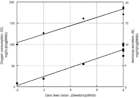
In addition to the hourly data of the four treatments of Figs.1and2, average daily data for four additional treatments are also provided by Zakes et al. (2006), two of them for the intermediate feed rations 0.2%/d and 0.5%/d. The daily means plotted in Fig.3show (1) that daily OC and AE are linearly related to the feed ration, and (2) that the scatter due to Fig. 2 Correlation between oxygen consumption and ammonia excretion. Hourly data of Zakes et al. (2006). Treatments as in Fig.1

feeding frequency (at the highest ration) is of the order of the scatter around the lines. Note, however, that both OC and AE seem to increase slightly with increased feeding frequency (not shown). The best-fit lines are

OC¼104:3þ9:92I R2¼0:96 ð2Þ

AE¼0:321þ1:063I R2¼0:94 ð3Þ where OC is in mg[O2]/(kg[BM]h) and AE is in mg[N]/(kg[BM]h), as before, and the

ration,Iis in g[feed]/(kg[BM]d). The intercepts on the ordinates (at zero ration) are, of course, similar to the corresponding rates of Fig.2.

The OC rates above rest level represent the SDA, which is referred to in this paper as ‘‘growth’’ respiration (Vahl 1984) in contrast with ‘‘maintenance’’ (rest) respiration (the intercept). SDA respiration is proportional to the feed ration (Jobling and Davies1980; Jobling1981). The linear dependence of specific growth on the feed ration (Brett1979; Boehlert and Yoklavich1983) is another expression of the same phenomenon, except that zero growth requires some energy to cover maintenance needs. Finally, Fig.3may also be viewed as a segment of the general saturation kinetic model (S curve) of Mercer (1982), namely, its ascending portion.

The dynamic model developed in this paper is intended to predict OC and AE for system design and operational purposes. It is meant to be parsimonious, namely, to have as small a number of parameters as possible. With this in mind and given the correlation between OC and AE (Fig.2), it is sufficient to develop a dynamic prediction model for OC and then calculate AE via the empirical Eq. 1. When more data become available, a separate process-based model for AE may become feasible.

Static model: partitioning of daily energy

Traditionally (Brafield and Llewellyn1982, p 19), the total gross energy contained in the consumed feed,C, is divided into four components, according to its final destination: (1) nondigestible, excreted as faeces and denoted here by F; (2) nitrogenous waste (urine, ammonia),A; (3) dissipated as respiratory heat,R; and (4) retained in the body (production, growth),G. Respiration may be further divided (Lupatsch et al.2003a) into (3a) mainte-nance respiration, RM, and (3b) growth respiration, RG. In this paper maintenance respiration is equated with rest respiration, whereas growth respiration, calculated as total respiration minus rest respiration, is thus equated with SDA.

Expressing consumed gross energy as a sum of its components,

C¼FþAþRMþRGþG; ð4Þ

four ratios are sufficient to specify its partitioning. A convenient choice in our case is

/¼ ðCFÞ=C energy digestibility ð5Þ

d¼A=C ammonia/consumed energy ð6Þ

b¼RG=G growth respiration/growth ð7Þ

q¼RG=RM growth respiration/maintenance respiration ð8Þ

is zero at zero growth and increases with ration size. By eliminatingF,A,RGandGfrom Eqs. 4–8, one obtains

q¼ b

1þb

ð/dÞ RM=C

RM=C

; ð9Þ

which, assuming thatRM,/,dandbare nearly invariant withC, shows (1) thatqis an increasing linear function of the ration C, and (2) that in view of Eqs. 7 and 8, growth respiration and growth are zero when the numerator is zero, namely, when

C¼RM=ð/dÞ; ð10Þ

where/–dis the fraction of feed consumed, C, available for maintenance and growth (metabolizable energy; Lucas1996, p 42). Furthermore, assuming that OC is proportional to total respiration,RT:RM+RG, and utilising Eqs. 8 and 9, OC is seen to be a linear function ofC, namely,

OC/RMþRG¼ 1

1þb½RMþbð/dÞC; ð11Þ

compatible with Fig.3 (Eq. 2). Assuming a linear relationship between AE and OC (Eq. 1), a linear dependence of AE onC, as in Fig.3, is also expected according to this simple model.

The values of the four parametersRM,/,dandbcan be obtained from the experimental results of Zakes et al. (2006), as will be shown later on. Once the parameter values are known, partitioning of total daily energy into its components (Eq. 4), for any ration beyond zero growth, may be obtained by using the following five relationships:

F

C¼1/ ð12Þ

A

C¼d ð13Þ

RM

C ¼ RM

C ð14Þ

RG

C ¼

b

1þb ð/dÞ

RM

C

ð15Þ

G C¼

1

1þb ð/dÞ

RM

C

: ð16Þ

The last equation shows that the conversion efficiency of feed into growth increases with ration size.

Dynamic model: simulating daily cycle

Compartments and fluxes

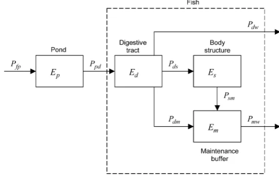
The contents of the compartments, E, are expressed in terms of metabolisable energy per unit biomass of fish (initially (/–d)C); and the fluxes, P, are fluxes of metabolisable energy. Interaction (input/output) with the environment of the modelled system is via Pfp, the time-dependent rate at which the daily ration is supplied to the pond (depending on treatment); Pdw (:RG), growth respiration; and Pmw (:RM), maintenance respiration. Ppd is the rate of flow into the active digestive tract (ingestion rate), andPdt=Pds+Pdw+Pdm, is the digestion (assimilation) rate, where

Pds is the flux of retained energy (fish growth), Pdw is the associated growth respi-ration and Pdm is energy for maintenance diverted to a temporary storage m. This buffer is used for maintenance respirationPmw, assumed to be uniform throughout the day. If the maintenance buffer compartment is empty, body tissue must be sacrificed viaPsmto support maintenance. This route is energetically more expensive due to the cost of growth respiration at a former stage.

The model has four state (cumulative) variables, namely, the contents Eof the four compartments. Simulation with the model requires, therefore, four initial values. The four state equations are, from Fig.4, as follows

dEp

dt ¼PfpPpd ð17Þ

dEd

dt ¼PpdPdtPpdPdwPdsPdm ð18Þ

dEs

dt ¼PdsPsm ð19Þ

dEm

dt ¼PdmþPsmPmw: ð20Þ

Flux rules

The various fluxes P may become limited by availability of substrate, by compartment capacity or by transfer capability. The various inhibition rules are as follows: Ingestion rate is limited by some maximum rate, Px_pd, by availability of feed in the pond,Ep[0, and when the digestive tract is full,Ed¼Exd:

Ppd¼Pxpd if Ep[0 and Ed\Exd ð21Þ

Ppd¼0 otherwise: ð22Þ

The digestion rate is formulated in the simplest possible manner, as being proportional to the substrate content of the digestive tract (Fa¨nge and Grove 1979, p 200; Lika and Papandroulakis2005):

Pdt¼aEd if Ed[0 ð23Þ

Pdt¼0 otherwise ð24Þ

whereais a digestive-rate constant. Direct transfer to the maintenance buffer is limited by the availability of substrate in the digestive tract and when the maintenance buffer is full:

Pdm¼kEd if Ed[0 and Em\Exm ð25Þ

Pdm¼0 otherwise; ð26Þ

wherekis a transfer-rate constant. Maintenance respiration rate is constant over the diurnal cycle:

Pmw¼RM: ð27Þ

Growth and growth respiration rates are limited by availability of substrate:

Pds¼1þ1bðPdtPdmÞ

Pdw¼_1þb_bðPdtPdmÞ

if PdtPdm[0 ð28Þ

Pds¼Pdw¼0 otherwise: ð29Þ

Transfer from structural tissue to maintenance takes place only when the maintenance buffer is empty:

Psm¼0 ifEm[0 ð30Þ

Psm¼RM otherwise: ð31Þ

Note that the specified digestion rate (Eq. 23) would result in an exponential decline of the content of the digestive tract once filling is stopped (e.g. after 18 h in Fig.1, Treatment 1; also He and Wurtsbaugh1993; Riche et al.2004). At the other end, when the digestive tract is full for a prolonged period of time ðEd¼ExdÞ, the OC attains a constant value (plateau):

PdwþPmw¼PdtPdmPdsþPmw¼ b

1þbðakÞE x

Justification

The justification for these rules is as follows:

1. The need for substrate (e.g.E[0) in Eqs. 21, 23, 25 and 28 is obvious. 2. Equation 21 assumes, intuitively, that there is a limit to the ingestion rate,Px

pd, and that the capacity of the digestive tract,Ex

d, is finite. In particular, the latter is responsible for the upper bound on OC and AE (plateau, Fig.1, Treatment 1). In a refined future version of the model, there may be an additional in-fish compartment, where ingested feed is temporarily stored before entering the active part of the digestive tract. 3. The simple proportionality of Eq. 23 is just a first approximation. The digestion

coefficientais probably a function of feed composition (SDA higher for protein-rich feed; Lucas1996, p 44).

4. As maintenance respiration goes on continuously, a certain energy reserve (of sizeEx m) must be available to bridge between feeding episodes. Siphoning off a fraction of the available digestion products (when available; Eq. 25) seems a simple way to gradually fill up the buffer compartment.

5. Maintenance respiration (Eq. 27) is assumed to be approximately constant, as indicated by the horizontal rest segments of Treatments 1 and 4 (Fig.1).

6. Equation 28 partitions the remaining energy (after fulfilling the need for maintenance) into its retained (growth) and respired components.

7. Long starvation periods may exhaust the reserve for maintenance. Some body tissue has then to be sacrifices to maintain the essential life processes (Eq. 31).

Parameters

The static (daily) model (Eqs. 4–16) has five parameters: RM, /,d andb, as well as a conversion factor,e, between oxygen and ration. The dynamic model (Eqs. 17–31), which considers only metabolisable energy, shows explicitly onlyRM(Eq. 31) andb(Eq. 28) but uses/anddto convert between gross energy and metabolisable energy andeto convert between feed and energy. Five additional parameters are required by the dynamic model, namely, the three maximum capacities:Px

pd,ExdandExm, and the two rate coefficients:aand

k; altogether ten parameters. The daily parameters RM, /, dand b, and the conversion factor,e, may be considered given to the dynamic model, leaving just five free parameters to be fitted (simultaneously) to the dynamic data.

The initial values of the state variables are determined as follows: The feed-energy content of the pond,Ep, and the energy content of the fish biomass,Es, are measurable, at least in principle (here E0

p¼0; E0s may be calculated from fish size, but not really required). The other two state variables,Ed(digestive tract) andEm(maintenance buffer), could be forced to be periodic if the treatment is assumed to be such (as in our case). If a transient process needs to be simulated, the two initial valuesE0dandEm0 may have to be themselves fitted (or measured, if feasible).

Energy partitioning results

Maintenance respiration rate is taken to be equivalent to the rest OC rate of Treatment 1 (Fig.1):

RM¼ 130 mg½O2=ðkg[BM]hÞ: ð33Þ

A value ford(Eq. 6) is obtained by estimatingAfrom the energy content of ammonia andC from the energy content of the consumed feed. The mean, for the three feeding treatments, of daily AE, is 226 mg[N]/(kg[BM]d), and the energy content of ammonia is 348 kJ/mol[N]. Hence,

A¼226 mg[N] kg[BM]d348

kJ mol[N]

1 14

mol[N] g[N] ¼5:6

kJ

kg[BM]d: ð34Þ

Using the given gross energy content of 20.8 kJ/g[feed], the consumed energy becomes

C¼8 g[feed] kg[BM]d20:8

kJ

g[feed]¼166 kJ

kg[BM]d: ð35Þ

The value ofdis thus

d¼5:6=166¼0:034: ð36Þ

The equivalence between oxygen and feed is obtained by dividing the energy content of feed with the oxycalorific equivalent, which for fish is often quoted as 13.6 kJ/g[O2] (after

Brett and Groves1979):

e¼20.8 kJ

g[feed]=13:6 kJ g[O2

¼1530mg[O2

g[feed]: ð37Þ

The parameters/ andbare obtained by equating the model expression for total res-piration (from Eq. 11)

RT RMþRG¼ 1

1þb½RMþbð/dÞC ¼ 1

1þb½130þbð/0:034ÞC; ð38Þ

with the linear fit of Eq. 2, in the form

RT ¼OC¼104:3þ9:92I¼104:3þ9:92 24C

e ¼104:3þ9:92 24C

1530: ð39Þ

The result is

b¼0:246 ð40Þ

/¼0:822: ð41Þ

The value for/compares favourably with the range provided by Lupatsch et al. (1997) and Jobling (1993). Regarding the value of b, an established sea-bream (Sparus aurata) model (Lupatsch, personal communication), uses a higher value, b = 0.39 and an in-between value ofb= 0.33 has been found for the tomato plant (Bertin and Gary

respiration level from starvation trials (Lupatsch et al.2003b), whereas our model utilises the 30% higher rest value (Fig.2). This changes the balance betweenRMandRG, reducing

RG:RT–RMin our case, hence resulting in a lower value ofb. Actually, if ourRMis to be lowered from 130 to 100 mg[O2]/(kg[BM]h) (rest to starvation), transferring 30 mg[O2]/

(kg[BM]h), about 6% of the energy, toRG, the result would beb= 0.39, the same as in the sea-bream model.

It is now possible to estimate the feed ration required to maintain exactly zero growth. Invoking Eq. 10 and using parameter values from Eqs. 33, 36, 37 and 41, the result is

I¼24C

e ¼

24RM

eð/dÞ¼

24130

1530 ð0:8220:034Þ¼2:59 g[feed]

kg[BM]d: ð42Þ

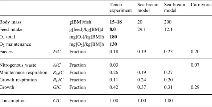
Using Eqs. 12–16 and the foregoing parameter estimates (Eqs. 33, 36, 40 and 41), the partitioning into the five energy components of Eq. 4, for ration 0.8%/d (Eq. 35), becomes

F:A:RM :RG:G¼0:18:0:03:0:26:0:11:0:42: ð43Þ

These estimated ratios are compared in Table1, with results obtained with the sea-bream model (also at 23C,Anot included), and with a representative partitioning for carnivorous fish (Brafield1985, p 258; tench and sea-bream are mainly carnivorous). Two sizes of sea bream are considered: 20 and 200 g, results for the latter being very similar to the general proportions for carnivores. The most significant differences between tench and sea-bream are: (1) Feed intake is much higher for sea bream. The sea-bream model assumes feeding to satiation, whereas the fish in the tench experiment were, apparently, underfed (only 0.8% of BM per day; see discussion below). Some of the difference may also be due to differing species and experimental procedures. (2) The ratio b =RG/G is considerably smaller for tench than for sea bream. This has just been explained by the difference in defining the termRMin the two models.

The parameter values estimated in the preceding paragraphs are based on data obtained with the 0.8%/d ration, plus some, presumably conservative, coefficients from the litera-ture. However, Eq. 9 makes it possible to partition the consumed energy for other rations

Table 1 Partitioning of daily energy: comparison between tench data and model results, sea-bream model results and representative partitioning for carnivorous fish (Brafield1985)

Tench experiment

Sea-bream model

Sea-bream model

Carnivores

Body mass g[BM]/fish 15–18 20 200

Feed intake g[feed]/kg[BM]d 8.0 29.1 12.1

O2total mg[O2]/kg[BM]h 180

O2maintenance mg[O2]/kg[BM]h 130

Faeces F/C Fraction 0.18 0.19 0.23 0.20

Nitrogenous waste A/C Fraction 0.03 0.07

Maintenance respiration RM/C Fraction 0.26 0.19 0.27

Growth respiration RG/C Fraction 0.11 0.24 0.20

Growth G/C Fraction 0.42 0.37 0.31 0.29

Consumption C/C Fraction 1.00 1.00 1.00

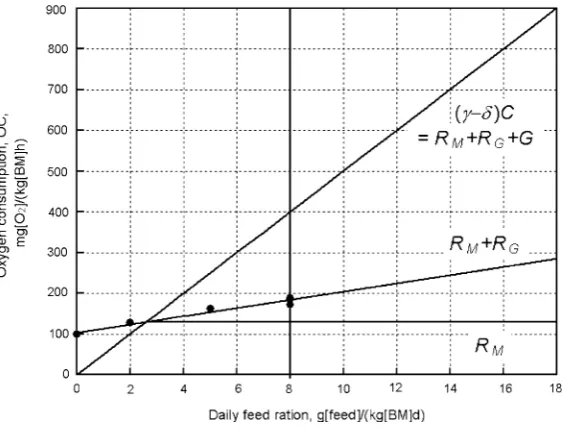
as well. Figure5(solid lines) shows the expected energy partitioning over a wide range of rations, from starvation to about the maximum the fish can consume (to be discussed later). It is assumed here thatRM(rest value) remains constant down to the zero-growth ration (evaluated in Eq. 42) and then decreases linearly down to the starvation OC level. Below the zero-growth ration, the fish draw on their reserves to support their livelihood. The predicted total respiration rate (Eq. 38), a linear function of the ration, is derived directly from the OC data of Fig.3(points).

Simulation results

The dynamic OC model has been fitted, by visual trial-and-error, to data of the three feeding treatments. The four ratios b,/,d ande and the respiration maintenance (rest) level,RM, were set according to the values leading to Eq. 43. The three capacitiesPx_pd,Ex_d

andEx

m, and the two rate coefficientsaandk, were adjusted, by fitting the dynamic data, to

Ex

d=C¼0:44,Exm=C¼0:09,Pxpd¼1:7 g[feed]/(kg[BM]h),a= 0.18 1/h andk= 0.054 1/ h. In other words, the effective capacity of the digestive tract is estimated at 0.44 of the daily energy consumption,C, alternatively 0.44·8 = 3.5 g[feed]/kg[BM], or 0.44·8· 1530 = 5355 mg[O2]/kg[BM]. The effective capacity of the maintenance buffer is

esti-mated at 0.09 of C, or 0.09· 8 = 0.7 g[feed]/kg[BM] (this is a lower bound value, as explained later in the discussion). The maximum ingestion rate is 1.7 g[feed]/(kg(BM)h), considerably less than the feeding rate of Treatments 1 and 2 (8/3 = 2.67 g[feed]/ (kg[BM]h)). The two transfer coefficients represent half-life times of about 6 h for digestion and about 19 h for the replenishment of the maintenance buffer. Note that the

Fig. 5 Oxygen equivalent of several energy components of Eq. 4, as a function of the feed ration, for the conditions of the Zakes et al. (2006) experiment.C,RM,RGandGare consumption, maintenance (rest) respiration, growth respiration (SDA) and growth, respectively.Solid lines represent model predictions.

fitted value,a= 0.18 1/h, is not far from 0.15 1/h, the value obtained for gastric evacuation rate of tilapia at 28C (Riche et al.2004).

The initial compartment capacities (initial state of the model) were taken to be the same for all treatments, specifically: E0

p¼0,E0s ¼0,Ed/C= 0.05 and Em/C= 0.04. Selecting separateEdandEmvalues for each treatment could improve the fit to some extent. The prediction of AE required two more parameters, namely, the coefficients of Eq. 1.

Figure6 shows the simulated OC and AE trajectories (lines) superimposed on the measured data (asterisks). The fit of AE is somewhat poorer than the fit of OC, reflecting the scatter in Fig.2and specifically the deviation of the top points. The qualitative fit is rather good, particularly the model’s ability to mimic the plateau of Treatment 1 and the concave and convex curvatures of the ascending and descending segments.

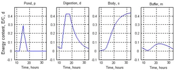
Figure7shows, for Treatment 1 (single feeding), the variation with time of the content of the four compartments of the model. There are no measured values for these variables. The first frame, representing the pond, shows how the difference between feeding rate and ingestion rate results in accumulation of noningested feed in the water, which starts to decrease only when feeding stops. Part of this temporary storage of feed may actually be inside the fish, awaiting admittance into the active part of the digestive tract. The active digestive tract (second frame) is seen to have a limited capacity (0.44 of the daily gross energy, dictated by the value ofExd). It fills up quickly and empties asymptotically to zero. Growth (third frame) starts soon after feeding, continues for the rest of the day and utilises about 0.42 of the daily gross energy (Eq. 43). The initial content of this compartment is arbitrary (here zero), as only the increment over the day is of interest. The maintenance buffer (last frame) fills up during feeding and later is consumed by maintenance respiration. Note that the digestion and buffer compartments return only approximately to their initial content at the end of the 24-h cycle. This is the result of selecting the same initial conditions for all treatments.

Table2summarises the partitioning of energy among the various utilisation categories. The ‘‘expected’’ partitioning is taken from Eq. 43. The model ensures exact partitioning to maintenance respiration, faeces and ammonia. The dynamic partitioning to growth (and growth respiration) is not exact, resulting in imperfect balance closure (equal to the changes in compartment contents over the cycle).

Discussion

Number of parameters

Models should not have redundant parameters. At first sight, this does not seem to be the case here, as some parameters are correlated (have a similar effect). For example,

increasing Ex

d, ora; ordecreasing k, all result in an elevated OC plateau (Eq. 32). Should some of the parameters, and the processes they represent, be eliminated from the model?

To illustrate the problem, let us considerEx

m, the maintenance buffer size. The last frame of Fig.7 shows that Em/C never exceeds 0.09. Any compartment size larger than that would result in exactly the same simulated trajectories and hence in the same goodness of fit. In other words, the second condition of Eq. 25 is always met, and the parameterEx

mmay be removed from the model. This conclusion is probably correct for cases involving daily periodicity, such as the current case. For a transitional problem, however, where Fig. 7 Simulated compartment energy contents (state variables) for feeding-treatment 1 in terms ofE/C, i.e. fraction of daily ration.Left to right: pond, digestive tract, body structure, maintenance buffer

Table 2 Summary table of energy partitioning obtained by simulation

Treatment 1 Treatment 2 Treatment 3 Expected Simulated Simulated Simulated

Faeces F/C 0.18 0.18 0.18 0.18

Nitrogenous waste A/C 0.03 0.03 0.03 0.03

Maintenance respiration RM/C 0.26 0.26 0.26 0.26

Growth respiration RG/C 0.10 0.12 0.10 0.11

Growth G/C 0.43 0.45 0.40 0.42

Discrepancy 0.00 –0.03 0.03 0.01

Consumption C/C 1.00 1.00 1.00 1.00

accumulation and/or depletion may continue for several days, the capacity of the buffer may become important. If the model is intended to be applied eventually to a wide range of feeding regimes, some of them extreme, Exm should be retained in the model. At the moment, only a lower bound on its value (Em/C = 0.09) can be set, but special long-term experiments may enable proper estimation of the effective buffer size. A similar argument might have been brought up regarding the capacity of the digestive tract,Ed/C. If Treat-ment 1 had been eliminated from the experiTreat-ment, the plateau (Fig.6, second frame) would not materialise, and the value ofEdx=C could not have been estimated.

The need for the other parameters can also be defended, claiming that, intuitively, they may have a quantifiable role under some feeding conditions:Px

pd, the maximum ingestion rate, intuitively represents a real property of the living organism. In the simulation, it affects the slope of the ascending segments of the OC in the first two treatments, where feeding rate,Pfp, exceeds ingestion rate,Ppd. The two rate coefficients seem also necessary:

acontrols the digestion rate (and probably depends on feed composition), andkpartitions energy to the maintenance buffer. Eliminating the maintenance buffer from the model by combining it with the structural compartment may result in a fair fit, but at the cost of excessive respiration (utilising complex body tissue for maintenance).

At this stage of model development, it seems that the rather limited biological content of the model should be preserved. More complete data sets could support better estimates of the parameters of both the static (based on daily totals) and dynamic (requiring hourly data) parts of the model.

Mimicking starvation

The flux rules (Eqs. 21–31) have been developed to predict the results of the three feeding treatments (Fig.6). If applied as is to the starvation treatment (Treatment 4, Fig.1), the predicted OC would be 130 mg[O2]/(kg[BM]h) rather than the measured 100 mg[O2]/

(kg[BM]h). As fed (active) fish do expend more energy at rest than do starving fish (Jobling1993; Zakes et al.2006), Eq. 31 could be modified to

Psm¼RsM; ð44Þ

and Eq. 27 to

Pmw¼RsM ð45Þ

whenever the maintenance buffer is empty. In Eqs. 44 and 45, the superscript sdenotes starvation andRs

M\RM. Starvation conditions imply that the buffer is empty all the time. Setting Rs

M¼100 mg[O2]/(kg[BM]h), the proper daily respiration for the starvation

treatment would be obtained, and a gradual increase of maintenance rate (from 100 to 130 mg[O2]/(kg[BM]h)), as in Fig.5, will result as the ration is increased from starvation

to zero growth. Note, however, that for rations in this range, Eq. 1 needs to be modified to prevent negative AE rates.

Maximum growth rate

Davies (1980), where the two highest rations (out of three) reached the same OC plateau, except that the decline started earlier for the smaller ration (as would be predicted by the current model).

If the digestive tract was completely full throughout the diurnal cycle, the model, via Eq. 32, would predict a constant digestion rate equivalent to OC of about 267 mg[O2]/

kg[BM]h (Fig.6, Treatment 1, plateau). From Eq. 15 and the values of the various parameters, the oxygen equivalent of the feed ration under these conditions is

C¼ð1þbÞRGþbRM

bð/dÞ ¼

1:246 ð267130Þ þ0:246130 0:246ð0:8220:034Þ ¼1046 mg½O2=ðkg[BM]hÞ;

ð46Þ

and the partitioning of energy (Eqs. 12–16) becomes

F:A:RM :RG:G¼0:18:0:03:0:12:0:13:0:54: ð47Þ

Assuming that the daily maintenance respiration,RM, is independent of ration, the ration could be increased, in view ofRMin Eqs. 43 and 47, by a factor of (0.26/0.12=) 2.2. The new ration, namely, 17.6 g[feed]/(kg[BM]d) (to be compared with Table1), would result, in view ofGin Eqs. 43 and 47, in a (2.2·0.54/0.42=) 2.83-fold increase in growth. It will also result in an improved feed conversion factor (C/G), namely, by a factor of (0.54/ 0.42=) 1.3. Note that the relationships of Fig.5 are extended to the maximum ration, 18 g[feed]/(kg[BM]d), on the assumption that the linear relationship (the model) persists. If the fish to be modelled cannot operate continuously at full capacity, a growth-limiting mechanism of some sort (another limiting link in the processing chain) or a time constraint (rest period) must be added to the model.

Temperature and size effects

The current model is limited to a certain size of a certain fish at a certain temperature (and a certain feed composition). It is well established that species, size and temperature have a significant effect on metabolic rates (Jobling 1993). For instance, Lupatsch and Kissil (1998; Eq. 3), express the rate of growth of fish as

dM dt /M

p_{expfqTg; ð48Þ}

whereMis size of fish,Tis water temperature andpandqare constant coefficients. The values of the coefficients for sea bream (Lupatsch, personal communication) are, to a first approximation, p =*0.5 and q=*0.06/K (similar to the commonly used value of

2001) and may be estimated from information for similar species. As an example, He and Wurtsbaugh (1993) foundq= 0.073/K for gut evacuation rate.

Carbon dioxide excretion

As carbon dioxide may reach toxic levels in aquaculture, it is important to predict its flux. As a first approximation, its rate of excretion (CE) is proportional to OC. Hence, it should be a simple matter to add CE to the model.

Reduction of peak loads

The high peaks of Treatment 1 are shown to decrease considerably by more frequent feeding (Figs.1and6). This is particularly evident in the AE rate. Figure3shows that at the feeding rate of Treatments 1–3 (8 g[feed]/(kg[BM]d)), the mean OC rate is about 180 mg[O2]/(kg[BM]h) and the mean AE rate is about 9 mg[N]/(kg[BM]h). The first is

about 0.75 of the peak value of Treatment 1 and the latter is about 0.36 of the AE peak. Uniform feeding may, therefore, reduce significantly the installed capacity of nitrification biofilters in dense fish cultures, where ammonia buffer capacity in the pond is small. Alternatively, if growth rate could be increased by increasing the ration, as indicated in the subsection ‘‘Maximum growth rate’’, equipment suitably sized for the peak of Treatment 1 would be sufficient for the faster-growing fish.

Model usefulness

A model is more useful the more general it is. This study is rather limited in scope. Only one of many cultivated fish species is considered, and only one set of data is available. Furthermore, some potentially valuable data, such as rate of growth and feed digestibility, are not provided in the Zakes et al. (2006) paper. At this early stage of development, the proposed model, with its rudimentary biological content, is only applicable to the condi-tions of the Zakes et al. (2006) study. Nevertheless, it is plausible that the simplifying assumptions of the model could also apply to other fish under different conditions. Those conditions are: (1) Feeding frequency has a negligible effect on daily respiration and growth (Fig.3). (2) Maintenance (rest) respiration rate is independent of the daily feed ration. (3) Maintenance respiration rate is constant over the daily cycle. (4) The processing capability of the digestive tract is constant throughout the daily cycle (no circadian rhythm). (5) The capacity (volume) of the digestive tract is limiting digestion rate and hence growth rate. (6) Oxygen consumption and AE are well correlated (Fig.2).

Conclusions

1. The model has two parts: (1) static, producing the daily partitioning of energy as a function of feed ration (Fig.5); and (2) dynamic, predicting the instantaneous behaviour (Fig.6). The static part may be useful for design purposes and the dynamic part for control purposes.

2. The dynamic model produces fair OC and AE predictions for the Zakes et al. (2006) experiment (Fig.6).

3. Limited additional data, such as growth rate, feed digestibility, maintenance needs of other fish sizes and at other temperatures, could extend considerably the scope of the model. Application to other fish species requires more experimental data.

Acknowledgement I am grateful to Ingrid Lupatsch of the National Center for Mariculture in Eilat, Israel, for providing me with the latest version of the sea-bream model and for helpful discussions and references on fish-feeding issues.

References

Azzaydi M, Madrid JA, Zamora S, Sanchez-Vazquez FJ, Martinez FJ (1998) Effects of three feeding strategies (automatic, ad libitum demand feeding and time-restricted demand feeding) on feeding rhythms and growth in European sea bass (Dicentrarchus labraxL.). Aquaculture 163:285–296 Belal IEH (2005) A review of some fish nutrition methodologies. Bioresour Technol 96:395–402 Bertin N, Gary C (1993) Evaluation d’un modele dynamique de croissance et de developpement de la tomate

(Lycopersicon esculentum Mill), TOMGRO, pour differents neveaux d’offre et de demande en assimilates. Agronomie 13:395–405

Boehlert GW, Yoklavich MM (1983) Effects of temperature, ration and fish size on growth of juvenile black rockfish,Sebastes melanops. Env Biol Fish 8(1):17–28

Boujard T, Jourdan M, Kentouri M, Divanach P (1996) Diel feeding activity and the effect of time-restricted self-feeding on growth and feed conversion in European sea bass. Aquaculture 139:117–127 Brafield AE (1985) Laboratory studies of energy budgets. In: Tytler P, Calow P (eds) Fish energetics: new

perspectives. Croom Helm, London, p 349

Brafield AE, Llewellyn MJ (1982) Animal energetics. Blackie, Glasgo, p 168

Brett JR (1979) Environmental factors and growth. In: Hoar WS, Randall DJ, Brett JR (eds) Fish physi-ology, vol VIII. Academic Press, New York, p 786

Brett JR, Groves TDD (1979) Physiological energetics. In: Hoar WS, Randall DJ, Brett JR (eds) Fish physiology, vol VIII. Academic Press, New York, pp 280–352

Chen W-M, Purser J, Blyth P (1999) Diel feeding rhythms of greenback flounderRhombosolea tapirina

(Gunter 1862): the role of light-dark cycles and food deprivation. Aquac Res 30:529–537

Eding EH, Kamstra A, Verreth JAJ, Huisman EA, Klapwijk A (2006) Design and operation of nitrifying trickling filters in recirculating aquaculture: a review. Aquacult Eng 34:234–260

Fa¨nge R, Grove D (1979) Digestion. In: Hoar WS, Randall DJ, Brett JR (eds) Fish physiology, vol VIII. Academic Press, New York, p 786

Foss A, Vollen T, Oiestad V (2003) Growth and oxygen consumption in normal and O2 supersaturated

water, and interactive effects of O2saturation and ammonia on growth in spotted wolffish (Anarhichas minorOfalsen). Aquaculture 224:105–116

De la Gandara F, Garcia-Gomez A, Jover M (2002) Effect of feeding frequency on the daily oxygen consumption rhythms in young Mediterranean yellowtails (Seriola dumerili). Aquacult Eng 26:27–39 Gillooly JF, Brown JH, West GB, van Savage M, Charnov EL (2001) Effects of size and temperature on

metabolic rate. Science 293:2248–2251

Guinea J, Fernandez F (1997) Effect of feeding frequency, feeding level and temperature on energy metabolism inSparus aurata. Aquaculture 148:125–142

He E, Wurtsbaugh WA (1993) An empirical model of gastric evacuation rates for fish and an analysis of digestion in piscivorous brown trout. Trans Amer Fish Soc 122:717–730

Jobling M (1981) The influences of feeding on the metabolic rate of fishes: a short review. J Fish Biol 18:385–400

Jobling M (1983) Towards an explanation of specific dynamic action (SDA). J Fish Biol 23:549–555 Jobling M (1993) Bioenergetics: feed intake and energy partitioning. In: Rankin JC, Jensen FB (eds) Fish

ecophysiology. Chapman & Hall, London, p 421

Jobling M, Davies PS (1980) Effects of feed on metabolic rate, and the specific dynamic action in plaice,

Pleuronectes platessaL. J Fish Biol 16:629–638

Knights B (1985) Energetics and fish farming. In: Tytler P, Calow P (eds) Fish energetics: new perspectives. Croom Helm, London, p 349

Knutsen I, Salvanes AGV (1999) Temperature-dependent digestion handling time in juvenile cod and possible consequences for prey choice. Mar Ecol Prog Ser 181:61–79

Lika K, Papandroulakis N (2005) Modeling feeding processes: a test of a new model for seabream (Sparus aurata) larvae. Can J Fish Aquat Sci 62:425–435

Lucas A (1996) Bioenergetics of aquatic animals. Taylor & Francis, London, p 169

Lupatsch I, Kissil GW (1998) Predicting aquaculture waste from gilthead seabream (Sparus aurata) culture using a nutritional approach. Aquat Living Resour 11(4):265–268

Lupatsch I, Kissil GW, Sklan D, Pfeffer E (1997) Apparent digestibility coefficients of feed ingredients and their predictability in compound diets for gilthead seabream,Spaurus aurataL. Aquac Nutr 3:81–89 Lupatsch I, Kissil GW, Sklan D, Pfeffer E (1998) Energy and protein requirements for maintenance and

growth in gilthead seabream (Spaurus aurataL.). Aquac Nutr 4:165–173

Lupatsch I, Kissil GW, Sklan D (2003a) Defining energy and protein requirements of gilthead seabream (Sparusaurata) to optimize feeds and feeding regimes. Israel J Aquac – Bamidgeh 55(4):243–257 Lupatsch I, Kissil GW, Sklan D (2003b) Comparison of energy and protein efficiency among three fish

species gilthead sea bream (Sparusaurata), European sea bass (Dicentrarchus labrax) and white grouper (Epinephelus aeneus): energy expenditure for protein and lipid deposition. Aquaculture 225:175–189 Mercer LP (1982) The quantitative nutrient-response relationship. J Nutr 112(3):560–566

Phillips TA, Summerfelt RC, Clayton RD (1998) Feeding frequency effects on water quality and growth of walleye fingerlings in intensive culture. Prog Fish-Cult 60(1):1–8

Pichavant K, Person-Le-Ruyet J, Le Bayon N, Severe A, Le Roux A, Boeuf G (2001) Comparative effects of long-term hypoxia on growth, feeding and oxygen consumption in juvenile turbot and European sea bass. J Fish Biol 59:875–883

Requena A, Fernandez-Borras J, Planas J (1997) The effects of a temperature rise on oxygen consumption and energy budget in gilthead seabream (Sparus aurata). Aquac Int 5:415–426

Riche M, Haley DI, Oetker M, Garbrecht S, Garling DL (2004) Effect of feeding frequency on gastric evacuation and the return of appetite in tilapiaOreochromis niloticus(L.). Aquaculture 234:657–673 Vahl O (1984) The relationship between specific dynamic action (SDA) and growth in the common starfish,

Asterias rubensL. Oecologia 61(1):122–125

Yager TK, Summerfelt RC (1994) Effects of feeding frequency on metabolism of juvenile walleye. Aquacult Eng 13:257–282

Zakes Z, Demska-Zakes K, Kata K (2003) Rates of oxygen consumption and ammonia excretion of juvenile Eurasian perchPera fluviatilisL. Aquac Int 11:277–288