Reliability-Constrained
Unit
Commitment
Considering
Interruptible Load Participation
F. Aminifar
*and M. Fotuhi-Firuzabad
*Abstract: From the optimization point of view, an optimum solution of the unit commitment problem with reliability constraints can be achieved when all constraints are simultaneously satisfied rather than sequentially or separately satisfying them. Therefore, the reliability constraints need to be appropriately formulated in terms of the conventional unit commitment variables. In this paper, the reliability-constrained unit commitment problem is formulated in a mixed-integer program format. Both the unit commitment risk and the response risk are taken into account as the probabilistic criteria of the operating reserve requirement. In addition to spinning reserve of generating units, interruptible load is also included as a part of operating reserve. The numerical studies using IEEE-RTS indicate the effectiveness of the proposed formulation. The obtained results are presented and the implementation issues are discussed. Two sensitivity analyses are also fulfilled to illustrate the effects of generating unit failure rates and interruption time of interruptible load.
Keywords: Interruptible Load, Response Risk, Spinning Reserve, Unit Commitment Risk.
Nomenclature1 Indices
k ,j ,
i Generating unit indices.
t Time period index.
Constants
t i
A Coefficient of the offered cost of unit i in period t.
i
DT Minimum down time of unit i (h). 0
i
F Number of periods unit i has been offline prior to the first period of the time span (h).
i
G Number of periods unit i must be initially online due to its minimum up time constraint (h).
) t (
ILmax Maximum value of interruptible load in period t (MW).
i
L Number of periods unit i must be initially offline due to its minimum down time constraint (h).
LT System lead time (h).
MT System margin time (h).
i
NL Number of segments of the offered cost of unit i.
min i
P Minimum power output of unit i (MW).
max i
P Maximum power output of unit i (MW).
t d
P System load demand in period t (MW).
Iranian Journal of Electrical & Electronic Engineering, 2007. * The Authors are with the Department of Electrical Engineering, Sharif University of Technology, Tehran, Iran.
E-mails: [email protected], [email protected].
t i
q Rate offered for spinning reserve by unit i in
period t ($/MWh). t
IL
r Rate offered for interruptible load in period t ($/MWh).
i
RD Ramp-down rate of unit i (MW/h).
i
RU Ramp-up rate of unit i (MW/h).
t
RMP Regulating margin percentile in period t (%).
i
SD Shutdown ramp rate of unit i (MW).
i
SU Startup ramp rate of unit i (MW).
t
Pr
S Specified unit commitment risk in period t.
t
Pr
SR Specified response risk in period t. t
, l i
S Price of block l of the offered cost of unit i in period t ($/MWh).
l i
T Upper limit of block l of the offered cost of unit i (MW).
i , 2 i , 1 ,U
U Unavailability of unit i at interruption time.
i , 3
U Unavailability of unit i at system lead time. r
i
U Unavailability of unit i at margin time. 0
i
U Number of periods unit i has been online prior to the first period of the time span (h).
i
UT Minimum up time of unit i (h).
) 0 (
Vi Initial commitment state of unit i.
i
λ Failure rate of unit i (f/h).
τ Interruption time of interruptible load (h).
Sets
I Set of indices of the generating units. T Set of the indices of the time periods.
Variables
1) Continuous Variables
) t (
IL Interruptible load contributed as operating reserve in period t (MW).
) t (
Pi Power output of unit i in period t (MW). )
t (
Pi Maximum available power output of unit i in
period t (MW). t
Pr Unit commitment risk in period t. t
Pr
R Response risk in period t.
) t (
Ri Spinning reserve contributed by unit i in period t (MW).
) t (
RMi Regulating margin contributed by unit i in period t (MW).
) t (
RM System regulating margin in period t (MW).
) t (
RRM System required regulating margin in period t (MW).
t , l i
δ Power produced in block l of the offered cost
of unit i in period t (MW). 2) Binary Variables
) t (
vi 1 if unit i is scheduled on in period t and 0 otherwise.
t j
α 1 if forced outage of unit j in period t contributes to the response risk state and 0 otherwise.
t jk
α 1 if forced outage of both units j and k in period t contributes to the response risk state and 0 otherwise.
t j , 1
σ 1 if, during interruption time and before contribution of interruptible load, forced outage of unit j in period t results in some loss of load and 0 otherwise.
t j , 2
σ 1 if, during interruption time and after
contribution of interruptible load, forced outage of unit j in period t results in some loss of load and 0 otherwise.
t j , 3
σ 1 if, during system lead time and after
contribution of interruptible load, forced outage of unit j in period t results in some loss of load and 0 otherwise.
t jk , 1
σ 1 if, during interruption time and before contribution of interruptible load, forced outage of both units j and k in period t results in some loss of load and 0 otherwise.
t jk , 2
σ 1 if, during interruption time and after
contribution of interruptible load, forced outage of both units j and k in period t results in some loss of load and 0 otherwise.
t jk , 3
σ 1 if, during system lead time and after
contribution of interruptible load, forced outage of both units j and k in period t results in some loss of load and 0 otherwise.
1 Introduction
In a restructured power system, there are two alternatives for dispatching energy and reserve services, namely, sequential dispatch and simultaneous dispatch. In sequential dispatch, energy is cleared first followed by clearing reserve. Theoretical analysis and practical experience have shown that sequential auction would result in price reversals. The simultaneous dispatch is to
clear the market for both energy and reserve at the same time [1, 2].
In a power system, operating reserve is needed to compensate unforeseen events such as sudden unit outages and/or unexpected increase in system demand [3]. Procurement and scheduling of operating reserve have important bearing in the unit commitment decision and dispatch, because they come at some cost [4]. Operating reserve includes different types of unit and system reserves such as spinning reserve, rapid-start units, and interruptible loads. Participation of demand side in the energy and reserve markets can reduce the total operating cost.
In most traditional unit commitment models as well as applications in market environment, operating reserve requirement is set using various deterministic criteria e.g. largest online unit, a fraction of demand, or some combinations of both them. Such criteria are easily understood and implemented but they do not reflect the stochastic nature of the system components. The probabilistic criteria, on the other hand, are more complex but represent the system outage probability and enable a solution of unit commitment to meet acceptable risk levels. The basic goal of a probabilistic technique is to maintain the system risk as close as possible but less than an allowable risk at all time periods. Operating reserve evaluation involves two distinctly different aspects. The first is unit commitment, in which the system operator decides which units and how many should be committed to satisfy the criterion which is referred to as the unit commitment risk. The second one, however, is associated with dispatch decisions and the evaluation of the response capability of those committed units to satisfy the other criterion which is referred to as the response risk [5]. Both sets of studies are necessary to obtain a complete picture of operating reserve assessment.
Over the last four decades, numerous techniques and
methods have been developed to incorporate
probabilistic reserve criteria in the formulation of the reserve-constrained unit commitment [5-11]. An iterative Lagrangian Relaxation (LR) approach was proposed in [6] to attack this problem. This approach consists of post-processing UC schedule to compute the level of risk for which customers are interrupted at each hour. If this risk is not less than a predefined value, then the SR requirements are adjusted, and the UC process is iterated until the target risk is attained. The proposed method by [6] has some drawbacks because it could be computationally intensive given that several UC runs may be required. In addition, it needs to calculate the capacity outage probability table (COPT) for each hour of all UC runs. Therefore, available methods lack the means of representing directly the probability distribution of discrete capacity outages within the unit commitment formulation. To get around this difficulty, reference [7] proposes a continuous approximation method to estimate the COPT explicitly within the
reserve-constrained UC as a function of the commitment variables. An approximation of this quantity is incorporated in the formulation of the UC optimization problem as an extra linear constraint using an exponential function whose parameters are system-dependent. The resulting schedule has an associated risk of disconnection below a predefined threshold.
Reference [8] proposes a pool market clearing process, including a probabilistic reserve determination. In [8], probabilistic reliability criteria such as loss of load probability (LOLP) and expected load not served (ELNS) were defined to set the reserve requirement. It introduced the notion of hybrid metrics based on the probabilities of loss of load due to single and double generating unit outages. The developed approach is accurate and reasonable with the capability to be presented as linear function of unit commitment integer and continuous variables.
References [9-11] attacked the unit commitment problem based on the priority list (PL). Although, these methods are able to consider multi-type operating reserves as well as uncertainty of forecasted load, they may result in sub-optimum solution and are not applicable in the restructured power systems.
In this paper, the unit commitment problem is formulated considering reliability constraints as the probabilistic criteria of the operating reserve requirements. From the optimization viewpoint, the better solution of a problem can be found when all the constraints are simultaneously considered rather than sequentially or separately satisfying them. But it needs appropriately modeling of the objective function and all constraints as a one mathematical block to be solved by the available powerful commercial solvers. Therefore, both unit commitment risk and response risk are modeled to be added to the conventional unit commitment problem. Besides the spinning reserve, interruptible load participation is considered as another reserve resource of the operating reserve. A number of case studies using IEEE-RTS are conducted to demonstrate the effectiveness of the proposed formulation.
The rest of the paper is organized as follows. Section 2 provides reliability models of generating unit and interruptible load. Problem formulation is presented in Section 3 and Section 4 expresses the mixed-integer formulation of the energy offered cost. In Section 5, the reliability evaluation technique is discussed. Section 6 presents the reliability constraints in terms of unit commitment variables. A number of case studies with the conclusions drawn from the analysis are presented in Sections 7 and 8, respectively.
2 Reliability Models of Generating Unit and Interruptible Load
Figure 1 shows a modified two-state model [5] used in operating reserve assessment for spinning units. It is assumed that the system lead time is relatively short
such that a failed unit can not be repaired or replaced during lead time. Under this condition, the time dependent probabilities of the operating and failing states for unit i can be approximated by (1) and (2), respectively.
t i i
t
ORR t e
1 ) failed (
P = − −λi ≅λ = (1)
t 1 e ) operating (
P i
t
i ≅ −λ
= −λ
(2)
where ORR is the outage replacement rate of unit i ti during lead time t [5].
Fig. 1 Two-state model of generating unit i used in operating reserve evaluation.
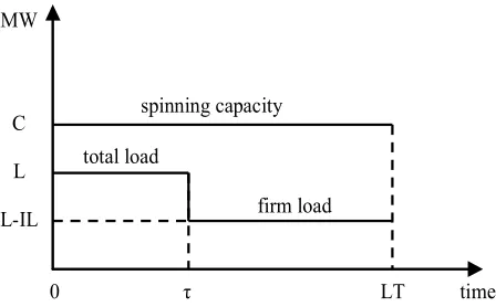
Interruptible load can be modeled as an equivalent generating unit with zero failure rate or considered as a load variation. In this paper, the load variation model is used for the purpose of computational analysis. This model is as shown in Fig. 2, where LT is the system lead time and τ is the interruption time of interruptible load. In this figure, L and C are respectively system load and generating units spinning capacity.
MW
L-IL C
L
0 τ LT
spinning capacity
firm load
time total load
Fig. 2 Load variation approach model for interruptible load.
3 Reliability-Constrained Unit Commitment
The objective function of the problem is formulated as follow:
∑∑
∈ ∈
+ +
T
t iI
t IL i t i i i t i
x [C (v(t),P(t)) qR (t) r IL(t)]
Min (3)
In (3), the total cost of utility including energy production, spinning reserve provision, and interruptible load participation over all decision variables x is minimized. In each time period t, each generator offer has two parts. The first one is to produce power Pi(t)at
an offered cost of C (vi(t),Pi(t))
t
i , and the second one
is to provide spinning reserve Ri(t) at an offered rate
of qit. Also, interruptible load offers rate of t IL
r to provide operating reserve IL(t) in time period t. This optimization problem is subject to different constraints as formulated in the following.
1) Generation Limits and Ramping Constraints [12]:
The generation limits of each unit for each period are set as follows. T t , I i ); t ( P ) t ( P ) t ( v
P i i i
min
i ≤ ≤ ∀ ∈ ∀ ∈ (4)
T t , I i ); t ( v P ) t ( P 0 i max i
i ≤ ∀ ∈ ∀ ∈
≤ (5)
Constraint (4) bounds the generation by the minimum power output and the maximum available power output of unit i in period t, which is a nonnegative variable bounded above by the unit maximum power output (5). VariablePi(t)is also constrained by ramp-up and startup
ramp rates (6), as well as by shutdown ramp rate (7).
T t , I i )]; t ( v 1 [ P )] 1 t ( v ) t ( v [ SU ) 1 t ( v RU ) 1 t ( P ) t ( P i max i i i i i i i i ∈ ∀ ∈ ∀ − + − − + − + − ≤ (6) T t , I i )]; 1 t ( v ) t ( v [ SD ) 1 t ( v P ) t (
P i i i i
max i i ∈ ∀ ∈ ∀ + − + + ≤ (7)
Furthermore, ramp-down limit is imposed on the power output by (8).
T t , I i )]; 1 t ( v 1 [ P )] t ( v ) 1 t ( v [ SD ) t ( v RD ) t ( P ) 1 t ( P i max i i i i i i i i ∈ ∀ ∈ ∀ − − + − − + ≤ − − (8)
It is worth to note that constraints (4)-(8) only include binary variables vi(t) and it is avoided defining extra
variables.
2) Spinning Reserve Constraint: To yield an accurate representation of the actual operation of generating units, the awarded spinning reserve of unit i should be restricted by hourly ramp-up limitation which is imposed on maximum available power output. Constraint (9) is included for this purpose.
T t , I i ); t ( P ) t ( P ) t ( R
0≤ i ≤ i − i ∀ ∈ ∀ ∈ (9)
3) Minimum Up and Down Time Constraints [12]:
The relevant expressions for minimum up time constraints are presented as follows.
I i ; 0 )] t ( v 1 [ i G 1 t
i = ∀ ∈
−
∑
= (10) 1 UT 24 ,..., 1 G t , I i )]; 1 t ( v ) t ( v [ UT ) n ( v i i i i i 1 UT t t n i i + − + = ∀ ∈ ∀ − − ≥∑
− + = (11) 24 ,..., 2 UT 24 t , I i ; 0 )]} 1 t ( v ) t ( v [ ) n ( v { i i i 24 t n i + − = ∀ ∈ ∀ ≥ − − −∑
= (12)where G is the number of initial periods during which i unit i must be online.G is mathematically expressed as i
)} 0 ( V ] U UT [ , 24 { Min G i 0 i i
i= − .
Constraints (10) is related to the initial status of the unit as defined by G . Constraint (11) is used for the i subsequent periods to satisfy the minimum up time constraint during all the possible sets of consecutive periods of size UT . Constraint (12) models the final i
1
UTi− periods in which if unit i is started up, it remains online until the end of the time span.
Analogously, minimum down time constraints are formulated as follows.
I i ; 0 ) t ( v i L 1 t
i = ∀∈
∑
= (13) 1 DT 24 ,..., 1 L t , I i )]; t ( v ) 1 t ( v [ DT )] n ( v 1 [ i i i i i 1 DT t t n i i + − + = ∀ ∈ ∀ − − ≥ −∑
− + = (14) 24 ,..., 2 DT 24 t , I i ; 0 )]} t ( v ) 1 t ( v [ ) n ( v 1 { i i i 24 t n i + − = ∀ ∈ ∀ ≥ − − − −∑
= (15)where L is the number of initial periods during which i unit i must be offline.L is mathematically expressed as i
)]} 0 ( V 1 ][ F DT [ , 24 { Min L i 0 i i
i= − − .
4) Interruptible Load Constraint: The third term in (3) is the cost of interruptible load participation. The amount of interruptible load is subject to the following limit: T t ); t ( IL ) t ( IL
0≤ ≤ max ∀ ∈ (16)
In this model, different amounts of interruptible load with relevant different costs can be easily taken into account.
5) Power Balance Constraint: Constraint (17) represents power balance in each time period.
T t ; P ) t (
P t
d I
i
i = ∀ ∈
∑
∈ (17)
6) Reliability Constraints: The blocks of the following formulation provide reliability constraints of problem.
T t ; Pr S
Prt≤ t ∀ ∈ (18)
T t ; Pr SR Pr
R t≤ t ∀ ∈
(19)
Constraint (18) expresses that in each period, the unit commitment risk must be less than a specified value which is appropriated for that period. Also, constraint (19) reveals that, the response risk for each period should be below the specified level.
4 Mixed-Integer Linear Model of Energy Offered Cost
The generating unit offered costs are usually presented by piecewise linear segments as illustrated in Fig. 3. The analytical mixed-integer representation of these segments is given below.
T t , I i
; S ) t ( v A )) t ( P ), t ( v (
C i
NL
1 l
t , l i t , l i i
t i i
i t i
∈ ∀ ∈ ∀
δ +
=
∑
= (20)
T t , I i ; P ) t ( v )
t (
P i imin
NL
1 l
t , l i i
i
∈ ∀ ∈ ∀ +
δ =
∑
=
(21)
T t , I i ; P
T min
i 1 i t , 1
i ≤ − ∀ ∈ ∀ ∈
δ (22)
1 NL ,..., 2 l , T t , I i ; T
T i
1 l i l i t , l
i ≤ − ∀ ∈ ∀ ∈ = −
δ −
(23)
T t , I i ; T
P NL 1
i max i t , NL
i i ≤ − i ∀ ∈ ∀ ∈
δ − (24)
i t
, l
i ≥0; ∀i∈I,∀t∈T,l=1,...,NL
δ (25)
where
T t , I i ; P S
A min
i t , 0 i t
i = ∀∈ ∀ ∈ (26)
Note that, the exponential startup cost and shutdown cost can be easily modeled without requiring any other variable [12].
t , 0 i
S
t , 3 i
S
t , 2 i
S
t , 1 i
δ
2,ti
δ
3,ti
δ
0
mini
P
T
i1T
i2P
imaxP
i(
t
)
t , 1 i
S
Fig. 3 Energy production offered cost of unit i in period t.
5 Reliability Evaluation Technique Considering Interruptible Load
As aforementioned earlier, operating reserve evaluation involves two distinctly different aspects, i.e. the unit commitment risk and the response risk. Both sets of studies are necessary to obtain a complete picture of operating reserve assessment.
5.1 Unit Commitment Risk
The unit commitment risk is associated with the assessment of which units to commit in any given period of time. The basis is to evaluate the probability of the committed generation just satisfying or failing to satisfy the expected demand during the time period that generation can not be replaced [5]. This time period is known as the lead time. In this paper for the simplicity, the system lead time is assumed to be one hour so that the reliability evaluation of each time period is not dependent on the commitment schedule of next periods. The case with system lead time more than one hour, is currently under development and will be presented in the near future.
In the presence of interruptible load with a short interruption notice time, the unit commitment risk in period t can be calculated as below:
T t ; Pr Pr Pr
Pr t
3 t 2 t 1
t= − + ∀ ∈
(27)
where for ∀i∈I,∀t∈T: t
1
Pr is calculated using τ =λ τ
i i
ORR and neglecting
interruptible load. t
2
Pr is calculated using τ =λτ
i i
ORR and including
interruptible load. t
3
Pr is calculated using ORR iLT LT
i =λ and including interruptible load.
5.2 Response Risk
The awarded amount of spinning reserve of units, i.e. )
t (
Ri , is restricted by hourly ramp rate of units, according to (9), to have an accurate representation of
the actual operation of the generating units. But, an assigned amount of spinning reserve must be available within a given time period to provide protection in the event of a sudden loss of generating capacity, or any other disturbance. This time period is referred to as the margin time and its actual value may vary from system to system. The margin time is defined as the time required to make necessary changes in generating unit output. The available generation change that can be achieved within a margin time is known as the regulating margin [5]. The margin time and the regulating margin are the two most important parameters in evaluating the response capability of generation system.
In the assessment of response capability, the constraint is that the total available response capacity of the committed units within a certain margin time must be greater than the required regulating margin plus system demand. Required regulating margin is determined as a specific percent of operating reserve. If the interruption time of interruptible load is less than margin time, the contribution of interruptible load should be taken into account in the response risk assessment. In this case, using load variation model, the system demand is reduced equal to awarded interruptible load.
6 Reliability Constraints as Explicit Functions of the Unit Commitment Variables
In the problem formulation, it is evident that constraints (4)-(17) are in linear manner. In Section 4, the offered cost C (vi(t),Pi(t))
t
i was also formulated in a
mixed-integer linear fashion. But, the reliability constraints of problem are not linear function of problem variables. In the following subsections, the unit commitment risk and the response risk formulations, due to single and double outages, are developed.
6.1 Unit Commitment Risk Formulation
The unit commitment risk in time period t, i.e. Pr , has t three terms as expressed in (27). Now, it is turn to define these three terms in terms of unit commitment variables.
1) Pr1t: It is formulated as below:
T t ; o Pr o Pr Pr J j k j , I k t jk , 1 t jk , 1 I j t j , 1 t j , 1 t
1 =
∑
σ +∑ ∑
σ ∀ ∈∈ < ∈
∈ (28)
In (28), we use a new set of binary variables T t , I j ; t j ,
1 ∀∈ ∀ ∈
σ , satisfying the following linear
inequalities.
∑
∑
∑
∑
∈ ≠ ∈ ∈ ≠ ∈ + − + ≤ σ ≤ + − I i max i j i , Ii i i
t d t j , 1 I i max i j i , I i i i t d P )) t ( R ) t ( P ( P 1 P )) t ( R ) t ( P ( P (29)
The binary variable t j , 1
σ models the presence or absence of some loss of load due to single outage random events in an explicit manner. Similarly, binary variables t
jk , 1
σ
are used in (28) for double generator outages for k j , I k ,
j ∈ < . These variables are characterized by (30).
∑
∑
∑
∑
∈ ≠ ∈ ∈ ≠ ∈ + − + ≤ σ ≤ + − I i max i k , j i , I i i i t d t jk , 1 I i max i k , j i , I i i i t d P )) t ( R ) t ( P ( P 1 P )) t ( R ) t ( P ( P (30)Also, in (28) the probabilities of single and double random events are as follows.
T t , I j ; ) U ) t ( v 1 ( U ) t ( v o Pr j i , I i i , 1 i j , 1 j t j ,
1 =
∏
− ∀∈ ∀ ∈≠ ∈ (31) T t , k j , I k ,j ; ) U ) t ( v 1 ( U ) t ( v U ) t ( v o Pr k , j i , I i i , 1 i k , 1 k j , 1 j t jk , 1 ∈ ∀ < ∈ ∀ − =
∏
≠ ∈ (32)where U is 1,i
t i
ORR of unit i within the interruption time, i.e. t=τ, as (33).
I i ;
U1,i =λi×τ ∀∈ (33)
2) Pr2t: It is formulated as below:
T t ; o Pr o Pr Pr J j k j , I k t jk , 2 t jk , 2 I j t j , 2 t j , 2 t
2 =
∑
σ +∑ ∑
σ ∀ ∈∈ < ∈ ∈ (34) where:
∑
∑
∑
∑
∈ ≠ ∈ ∈ ≠ ∈ + − − + ≤ σ ≤ + − − I i max i j i , I i i i t d t j , 2 I i max i j i , Ii i i
t d P )) t ( R ) t ( P ( ) t ( IL P 1 P )) t ( R ) t ( P ( ) t ( IL P (35)
∑
∑
∑
∑
∈ ≠ ∈ ∈ ≠ ∈ + − − + ≤ σ ≤ + − − I i max i k , j i , Ii i i
t d t jk , 2 I i max i k , j i , I i i i t d P )) t ( R ) t ( P ( ) t ( IL P 1 P )) t ( R ) t ( P ( ) t ( IL P (36)
The probabilities of single and double random events are similar to probabilities used in t
1 Pr .
3) Pr3t: It is formulated as below:
T t ; o Pr o Pr Pr J j k j , I k t jk , 3 t jk , 3 I j t j , 3 t j , 3 t
3 =
∑
σ +∑ ∑
σ ∀ ∈∈ < ∈
∈ (37)
where σt3,jand t
jk , 3
σ are respectively equal to σt2,jand t
jk , 2
σ . But, the probabilities of single and double random events are as below:
T t , I j ; ) U ) t ( v 1 ( U ) t ( v o Pr j i , I i i , 3 i j , 3 j t j ,
3 =
∏
− ∀∈ ∀ ∈≠ ∈ (38) T t , k j , I k , j ; ) U ) t ( v 1 ( U ) t ( v U ) t ( v o Pr k , j i , I i i , 3 i k , 3 k j , 3 j t jk , 3 ∈ ∀ < ∈ ∀ − =
∏
≠ ∈ (39)where U is 3,i
t i
ORR of unit i within the system lead time which is one hour in this paper, as (40).
I i ; 1
U3,i =λi× ∀ ∈ (40)
Note that the above expressions explicitly describe the unit commitment risk in terms of unit commitment variables, albeit in a nonlinear manner. Thus, these formulas need to be converted into a linear fashion.
6.2 Response Risk Formulation
In this paper, a new set of variables is used to satisfy the response risk constraint. Variable RMi(t) is the amount of regulating margin contributed by unit i in time period t. Although this variable does not exist in the objective function, but it is used in the response reliability constraint. The amount of regulating margin of unit i must be restricted above by unit’s awarded spinning reserve according to (41). Also, because the regulating margin is the available capacity during margin time, constraint (42) is included. System regulating margin is the sum of regulating margins of all online units as (43). Equation (44) determines the required regulating margin of each time period. In (44), RMP is representative of t a specific percent of operating reserve as the required
regulating margin and can vary from hour to hour according to reliability cost/worth surveys.
T t , I i ); t ( R ) t ( RM
0≤ i ≤ i ∀∈ ∀ ∈ (41)
T t , I i ; MT RU ) t (
RMi ≤ i⋅ ∀ ∈ ∀ ∈ (42)
T t ); t ( RM ) t ( RM I i
i ∀ ∈
=
∑
∈ (43) T t )); t ( IL ) t ( R ( 100 RMP ) t ( RRM I i i t ∈ ∀ + =∑
∈ (44)The response risk in time period t, i.e. RPrt, can be formulated as follow due to only single and double outages. T t ; o Pr R o Pr R Pr R J j k j , I k t jk t jk I j t j t j
t = α + α ∀ ∈
∑ ∑
∑
∈ < ∈ ∈ (45)In (45), we use a new set of binary variables
T t , I j ; t
j ∀∈ ∀ ∈
α , satisfying the following linear
inequalities.
∑
∑
∑
∑
∈ ≠ ∈ ∈ ≠ ∈ + − − + + ≤ α ≤ + − − + I i max i j i , I i i i t d t j I i max i j i , Ii i i
t d P )) t ( RM ) t ( P ( ) t ( IL ) t ( RRM P 1 P )) t ( RM ) t ( P ( ) t ( IL ) t ( RRM P (46)
The binary variable αtj models residing of generation system in the risk state from response analysis viewpoint, due to single outage random events. Similarly, binary variables αtjk are used in (45) for double generator outages for j,k∈I,j<k. These variables are characterized by (47).
∑
∑
∑
∑
∈ ≠ ∈ ∈ ≠ ∈ + − − + + ≤ α ≤ + − − + I i max i k , j i , Ii i i
t d t jk I i max i k , j i , I
i i i
t d P )) t ( RM ) t ( P ( ) t ( IL ) t ( RRM P 1 P )) t ( RM ) t ( P ( ) t ( IL ) t ( RRM P (47)
It should be noted that if the interruption time of interruptible load is equal to or more than margin time, the IL(t) must be omitted in (46) and (47). In (45) the probabilities of single and double random events are as follows.
T t , I j ; ) U ) t ( v 1 ( U ) t ( v o Pr R
j i
, I i
r i i r
j j t
j=
∏
− ∀∈ ∀ ∈≠
∈ (48)
T t , k j , I k , j
; ) U ) t ( v 1 ( U ) t ( v U ) t ( v o Pr R
k , j i
, I i
r i i r
k k r j j t j
∈ ∀ < ∈ ∀
−
=
∏
≠ ∈
(49)
where Uri is the unavailability of unit i within margin time as presented in (50).
I i ; MT
U i
r
i =λ × ∀∈ (50)
Similar to the unit commitment risk formulas, these expressions are not in a linear manner because they include product of binary variables. But they can be converted into linear expressions. Reference [8] has the details.
7 Numerical Studies
To illustrate the effectiveness of the proposed formulation, a set of case studies are conducted here using IEEE-RTS without hydro generation. The system has 24 thermal units and 2 nuclear units. The piecewise linear offered cost of units are constructed based on the incremental heat rate data (Table 9, [13]) and the following fuel prices: 3.884 $/MBTu for FO6 oil, 6.340 $/MBTu for FO2 oil, 1.209 $/MBTu for coal and 1.584 $/MBTu for the nuclear fuel [8]. For simplicity, it is assumed that all units offer reserve at rates qit equal to 10% of their higher incremental cost of producing energy. Data of units ramp restrictions and minimum up/down time limits are from Table 10, [13]. Reliability data of units were extracted from Table 6, [13]. Power generated by units committed at t=0 was assumed to be given by the economic dispatch of the committed units for the first period for a load level of 1500 MW. Hourly load distribution is similar to a summer weekday in Table 4, [13] with 2300 MW peak load.
The upper bound of interruptible load is equal to 100 MW and its offered rate rILt is assumed to be 3 $/MWh for all time periods. The system lead time, margin time and interruption time of interruptible load are respectively assumed to be 1 hour, 15 minuets, and 10 minutes. The regulating margin percentile, i.e. RMP , t is assumed to be 30% for all time periods.
In order to discuss the efficiency of the proposed formulation in detail, the following three cases are carried out:
• Case 1: Consider 10% of hourly load as a deterministic criterion for operating reserve requirement.
• Case 2: Consider SPrt =0.002as a probabilistic criterion for operating reserve requirement.
• Case 3: Consider SPrt =0.002 and
002 . 0 Pr
SR t = as probabilistic criteria for
operating reserve requirement.
The model has been implemented on a hp pavilion zt3000 with a processor at 1.60 GHz and 512 MB of RAM memory using the MIP solver CPLEX in GAMS [14] environment. In CPLEX, an optimality parameter can be specified to decide whether to find the optimal solution or to quickly obtain a suboptimal solution. In these case study, the execution of CPLEX was stopped when the value of the objective function was within 0.5% of the optimal solution.
Case 1: In this case, both unit commitment risk and response risk constraints are inactive. However, to provide a practical situation of power system operation, a fraction of hourly load is considered as a deterministic operating reserve criterion. The daily operating cost is 604,944 $ which includes costs of energy production, spinning reserve provision, and interruptible load participation. In this case, the maximum values of the unit commitment risk and the response risk are respectively equal to 0.00685 and 0.0035.
Case 2: In this case, only the constraint of the unit commitment risk is active and the response risk constraint is relaxed. The daily operating cost is 621,388 $ which is increased significantly versus case 1. The specified value of the unit commitment risk is set on 0.002 which is less than one third of its value in the case 1. In a comparison with first case results, more spinning reserve and interruptible load are purchased by system operator to reduce the system unit commitment risk. Therefore, this results in the response risk decrease as its maximum value reduces to 0.0017.
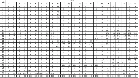
Case 3: Both unit commitment risk and response risk constraints are active and satisfied in this case. The specified values of the unit commitment risk and the response risk are respectively set on 0.002 and 0.001. With the stopping criterion of 0.5%, the execution time is 243 seconds to achieve a solution with the daily operation cost of 630,275 $ which is the highest among all cases. Table I shows the power dispatches of generating units. The expensive units 1-9, 14-16, and 21-23 are not committed at certain hours in order to minimize the operating cost. It can be seen that all system and units constraints like minimum up/down time limits and ramp rate restrictions are completely satisfied.
Table II presents the awarded spinning reserve of generating units as well as the purchased amount of interruptible load. As it can be observed, in 22 hours the maximum amount of interruptible load are purchased since it provides economical operating reserve. Spinning reserve of generating units, on the other hand, has somewhat unavailability but the probability of
having IL MW of load interrupted at the lead time τ, if required, is absolutely unity.
To illustrate the impact on the operating cost of interruptible load participation, consider a case without any interruptible load. Thus, spinning reserve is only resource which can be used to operate the system within acceptable levels of the unit commitment risk and the response risk. In this case, the daily operating cost is
635,780 $ which shows about 0.8% increase versus the operating cost of case with interruptible load participation. It is worth noting that the revenue obtained from participation of interruptible loads is dependent on many factors such as spinning reserve offered costs, interruptible load offered costs, and interruption time.
Table 1 Power dispatches of generating units.
1 2 3 4 5 6 7 8 9 10 11 12 13 14 15 16 17 18 19 20 21 22 23 24
1 0 0 0 0 0 0 0 0 0 2.4 2.4 2.4 2.4 0 0 0 0 0 0 0 0 0 0 0
2 0 0 0 0 0 0 0 0 0 0 0 0 0 0 0 0 0 0 0 0 0 0 0 0
3 0 0 0 0 0 0 0 0 0 2.4 2.4 2.4 2.4 0 0 0 0 0 0 0 0 0 0 0
4 2.4 2.4 2.4 2.4 0 0 0 0 0 2.4 2.4 2.4 2.4 0 0 0 0 0 0 0 0 0 0 0
5 0 0 0 0 0 0 0 0 0 2.4 2.4 2.4 2.4 0 0 0 0 0 0 0 0 0 0 0
6 0 0 0 0 0 0 0 0 0 0 0 0 0 0 0 0 0 0 0 0 0 0 0 0
7 0 0 0 0 0 0 0 0 0 15.8 0 0 0 0 0 0 0 0 0 0 0 0 0 0
8 0 0 0 0 0 0 0 0 0 0 0 0 0 0 0 0 0 0 0 0 0 0 0 0
9 0 0 0 0 0 0 0 0 0 0 0 0 0 0 0 0 0 0 0 0 0 0 0 0
10 60.8 60.8 60.8 38 38 38 38 60.8 60.8 76 76 76 76 76 76 76 76 76 60.8 60.8 60.8 60.8 60.8 60.8 11 60.8 46 60.8 38 38 38 38 60.8 60.8 76 76 76 76 76 76 76 76 76 60.8 60.8 60.8 60.8 60.8 60.8 12 60.8 46 60.8 38 38 38 38 60.8 60.8 76 76 76 76 76 76 76 76 62.3 60.8 60.8 60.8 60.8 60.8 60.8 13 60.8 54.8 60.8 38 38 50 38 60.8 60.8 76 76 76 76 76 76 76 66 60.8 60.8 60.8 60.8 60.8 60.8 60.8
14 0 0 0 0 0 0 0 0 25 25 25 47.4 25 50 50 25 25 0 0 0 0 0 0 0
15 0 0 0 0 0 0 0 0 0 25 49.4 50 50 50 50 38 25 25 25 0 0 0 0 0
16 0 0 0 0 0 0 0 25 25 35.6 50 50 49.4 50 50 25 25 0 0 0 0 0 0 0
17 155 155 155 155 155 155 155 155 155 155 155 155 155 155 155 155 155 155 155 155 155 155 155 113.9
18 155 155 108.5 155 138 155 155 155 155 155 155 155 155 155 155 155 155 155 155 155 155 155 155 155
19 155 155 155 155 138 155 155 155 155 155 155 155 155 155 155 155 155 155 155 155 155 155 155 113.9
20 155 155 108.5 126.3 155 155 155 155 155 155 155 155 155 155 155 155 155 155 155 155 155 155 155 113.9
21 0 0 0 0 0 0 0 0 0 0 0 0 0 0 0 0 0 68.9 68.9 68.9 68.9 68.9 68.9 68.9
22 0 0 0 0 0 0 0 0 0 0 0 0 0 0 0 0 0 0 68.9 68.9 68.9 68.9 68.9 68.9
23 0 0 0 0 0 0 0 0 0 0 68.9 68.9 68.9 76 76 68.9 68.9 68.9 68.9 68.9 68.9 68.9 0 0
24 350 350 350 342.2 350 350 350 350 350 350 350 350 350 350 350 350 350 350 280 350 350 350 350 350
25 101.4 100 108.5 100 100 100 171.4 155 400 400 400 400 400 400 400 400 400 400 363.9 400 375.9 398.9 249.9 314.1
26 155 100 102.9 100 100 100 178.5 354.8 337.8 400 400 400 400 400 400 400 400 400 400 295.9 320 320 400 113.9
Hours Units
Table 2 Awarded spinning reserve and interruptible load.
1 2 3 4 5 6 7 8 9 10 11 12 13 14 15 16 17 18 19 20 21 22 23 24
1 0 0 0 0 0 0 0 0 0 6.8 0 0 0 0 0 0 0 0 0 0 0 0 0 0
2 0 0 0 0 0 0 0 0 0 0 0 0 0 0 0 0 0 0 0 0 0 0 0 0
3 0 0 0 0 0 0 0 0 0 9.6 0 0 0 0 0 0 0 0 0 0 0 0 0 0
4 7 0 0 0 0 0 0 0 0 9.6 0 0 0 0 0 0 0 0 0 0 0 0 0 0
5 0 0 0 0 0 0 0 0 0 9.6 0 0 0 0 0 0 0 0 0 0 0 0 0 0
6 0 0 0 0 0 0 0 0 0 0 0 0 0 0 0 0 0 0 0 0 0 0 0 0
7 0 0 0 0 0 0 0 0 0 0 0 0 0 0 0 0 0 0 0 0 0 0 0 0
8 0 0 0 0 0 0 0 0 0 0 0 0 0 0 0 0 0 0 0 0 0 0 0 0
9 0 0 0 0 0 0 0 0 0 0 0 0 0 0 0 0 0 0 0 0 0 0 0 0
10 15.2 15.2 15.2 30 0 30 0 15.2 15.2 0 0 0 0 0 0 0 0 0 15.2 15.2 15.2 15.2 15.2 15.2
11 15.2 30 15.2 30 0 15 0 15.2 15.2 0 0 0 0 0 0 0 0 0 15.2 15.2 15.2 15.2 15.2 15.2
12 15.2 30 15.2 30 0 0 0 15.2 15.2 0 0 0 0 0 0 0 0 13.7 15.2 15.2 15.2 15.2 15.2 15.2
13 15.2 21.2 15.2 30 0 0 0 15.2 15.2 0 0 0 0 0 0 0 9.9 15.2 15.2 15.2 15.2 15.2 15.2 15.2
14 0 0 0 0 0 0 0 0 52 75 21.4 52.5 71.9 29 50 75 75 0 0 0 0 0 0 0
15 0 0 0 0 0 0 0 0 0 75 50.5 50 50 50 50 21.9 37 41.1 68.1 0 0 0 0 0
16 0 0 0 0 0 0 0 15.4 75 64.4 50 19.4 0 50 29 75 0 0 0 0 0 0 0 0
17 0 0 0 0 0 0 0 0 0 0 0 0 0 0 0 0 0 0 0 0 0 0 0 41
18 0 0 0 0 0 0 0 0 0 0 0 0 0 0 0 0 0 0 0 0 0 0 0 0
19 0 0 0 0 0 0 0 0 0 0 0 0 0 0 0 0 0 0 0 0 0 0 0 41
20 0 0 0 0 0 0 0 0 0 0 0 0 0 0 0 0 0 0 0 0 0 0 0 26.2
21 0 0 0 0 0 0 0 0 0 0 0 0 0 0 0 0 0 51.9 45 45 45 0 44.1 45
22 0 0 0 0 0 0 0 0 0 0 0 0 0 0 0 0 0 0 45 45 40.1 63.1 45 0
23 0 0 0 0 0 0 0 0 0 0 128 128 128 121 121 128 128 128 45 45.1 0 45 0 0
24 0 0 0 7.8 0 0 0 0 0 0 0 0 0 0 0 0 0 0 0 0 0 0 0 0
25 53.6 55 0 26.3 197.1 55 0 0 0 0 0 0 0 0 0 0 0 0 36 0 24 1.1 0 3.4
26 0 55 52.1 26.3 0 121.4 221.4 45.2 62.2 0 0 0 0 0 0 0 0 0 0 0 80 80 0 0
IL 100 15 42 100 100 100 100 100 100 100 100 100 100 100 100 100 100 100 100 100 100 100 100 100 Hours
Units
Fig. 4 Variation in the daily operating cost versus unit failure rates.
7.1 Effect of Generating Unit Failure Rates
In the given levels of the unit commitment risk and the response risk, the solution of the reliability-constrained unit commitment problem depends on many factors of which one of them is generating unit failure rate. This factor has no effect on the solution based on the deterministic criteria and the system will, therefore, face different risk levels with changes in the generating unit failure rates.
Assume that the generating unit failure rates change by an assigned factor. Fig. 4 illustrates the variation of the daily operating cost versus different values of multiplication factor from 0.1 to 1.5. As expected, the daily operating cost increases as the generating unit failure rates increase. In this figure, as it can be seen, the daily operating costs for both multiplication factors of 0.1 and 0.2 are equal to 592,577 $. Because in these cases, the awarded amounts of spinning reserve and interruptible load are equal to zero and both the unit commitment risk and the response risk are naturally less than their specified values. However, for multiplication factor more than 0.2, some amount of operating reserve must be purchased by system operator to satisfy the reliability constraints.
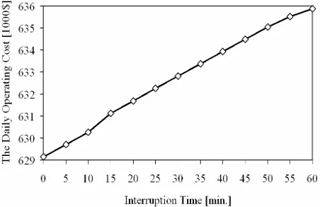
Fig. 5 Variation in the daily operating cost versus interruption time of interruptible load.
7.2 Effect of Interruption Time of Interruptible Load
In practice, a short notice time is agreed between system operator and interruptible load. This time is referred to as interruption time by most literatures. System operator must inform the owner of interruptible load within this short notice time if interruption is required. Interruption time is one of the influencing factors on the solution of reliability-constrained unit commitment problem. So, the impact of this factor is investigated here. Figure 5 illustrates variation of the daily operating cost versus increase of interruption time from 0 to 60 minutes. It should be noted that for interruption time equal to or more than 15 minutes (system margin time), interruptible load should not be included in the formulation of response risk constraint.
As it can be seen from Fig. 5, the increase of interruption time, as expected, results in growth of daily operating cost. The daily operating cost associated with interruption time of 10 minutes is 630,275 $ which is equal to the result of case 3. Also, the daily operating cost associated with interruption time of 60 minutes is equal to 635,780 $ which is, as expected, correspondent with the drawn conclusion in the last paragraph of case 3 , i.e. without participation of interruptible load. It is observed from Fig. 5 that increasing rate of curve between 10 and 15 minutes is slightly more than that of other intervals. The reason is that for interruption time less than 15 minutes, the participation of interruptible load can influence both unit commitment risk and response risk constraints. In contrast, for interruption time equal to or more than 15 minutes, the participation of interruptible load can only influence the unit commitment risk.
8 Conclusion
Probabilistic criteria provide a comprehensive and realistic evaluation of the operating reserve by incorporating the stochastic nature of system components. In this paper, a mixed-integer formulation has been developed for the reliability-constrained unit commitment problem. This formulation possesses two advantages: one is that it behaves in a manner consistent with probabilistic criteria such as unit commitment risk and response risk; second, its mathematical form is compatible with powerful MIP tools. The effectiveness of the proposed formulation has been manifested using different case studies. It has been concluded that, participating of interruptible load can reduce the daily operating cost while satisfying the given levels of reliability criteria. Sensitivity analysis on the generating unit failure rates revealed that, the daily operating cost increases as the generating unit failure rates are grown.
References
[1] Oren S., “Auction design for ancillary reserve
products,” in Proceeding IEEE Power
Engineering Society Summer Meeting, 2002, Vol. 3, pp. 1238–1239.
[2] Xia L. M., Gooi H. B., and Bai J., “Probabilistic spinning reserves with interruptible loads,” in
Proceeding IEEE Power Engineering Society General Meeting, Jun. 2004, Vol. 1, pp. 146–152. [3] Wood A. J. and Wollenberg B. F., Power generation, operation, and control, 2nd ed. New York: Wiley, 1996.
[4] Shahidehpour M., Yamin H., and Li Z., Market operations in electric power systems: forecasting, scheduling, and risk management. Piscataway, NJ: IEEE-Wiley-Interscience, 2002.
[5] Billinton R. and Allan R.N., Reliability evaluation of power systems, 2nd ed. New York: Plenum, 1996.
[6] Gooi H. B., Mendes D. P., Bell K. R. W., and Kirschen D. S., “Optimal scheduling of spinning reserve,” IEEE Transactions on Power Systems, Vol. 14, No. 4, pp. 1485–1492, Nov. 1999.
[7] Chattopadhyay D. and Baldick R., “Unit
commitment with probabilistic reserve,” in
Proceeding IEEE Power Engineering Society Winter Meeting, 2002, pp. 280– 285.
[8] Bouffard F. and Galiana F., “An electricity market with a probabilistic spinning reserve criterion,” IEEE Transactions on Power Systems, Vol. 19, No. 1, pp. 300–307, Feb. 2004.
[9] Billinton R. and Fotuhi-Firuzabad M., “A basic framework for generating system operating health analysis,” IEEE Transactions on Power Systems, Vol. 9, No. 3, pp. 1610–1617, Aug. 1994.
[10] Billinton R. and Fotuhi-Firuzabad M.,
“Generating system operating health analysis considering stand-by units, interruptible load and postponable outages,” IEEE Transactions on Power Systems, Vol. 9, No. 3, pp. 1618–1625, Aug. 1994.
[11] Billinton R. and Fotuhi-Firuzabad M., “A reliability framework for generating unit commitment,” Electric Power System Research, Vol. 56, pp. 81–88, 2000.
[12] Carrion M. and Arroyo J. M., “A computationally efficient mixed-integer linear formulation for the
thermal unit commitment problem,” IEEE
Transactions on Power Systems, Vol. 21, No. 3, pp. 1371–1378, Aug. 2006.
[13] Reliability Test System Task Force, “The IEEE reliability test system -1996,” IEEE Transactions on Power Systems, Vol. 14, No. 3, pp. 1010– 1020, Aug. 1999.
[14] Rosenthal R. E., GAMS: a user’s guide. Washington, D.C.: GAMS Development Corp., 2006.
Farrokh Aminifar received the
B.Sc. (Hon.) degree in electrical engineering from Iran University of Science and Technology, Tehran, Iran, in 2005 and M.Sc. (Hon.) degree in electrical engineering from Sharif University of Technology, Tehran, Iran, in 2007 where he is currently working toward the Ph.D. degree. His research interests include power system reliability, optimization, operation, and economics.
Mahmud Fotuhi-Firuzabad was
born in Iran. He obtained B.Sc. and M.Sc. degrees in electrical engineering from Sharif University of Technology and Tehran University in 1986 and 1989 respectively and M. S. and Ph.D. degrees in electrical engineering from University of Saskatchewan in 1993 and 1997 respectively. Dr. Fotuhi-Firuzabad worked as a postdoctoral fellow in the Department of Electrical Engineering, University of Saskatchewan from Jan. 1998 to Sep. 2000 and from Sep. 2001 to Sep. 2002 where he conducted research in the area of power system reliability. He worked as an assistant professor in the same department from Sep. 2000 to Sep. 2001. He joined the Department of Electrical Engineering at Sharif University of Technology in Sep. 2002. Presently he is the head of Department of Electrical Engineering, Sharif University of Technology. He is a member of Center of Excellence in Power System Management and Control in Sharif University of Technology, Tehran, Iran.