Please cite this article as: A. Sadati, R. Tavakkoli-Moghaddam, B. Naderi, M. Mohammadi, Solving a New Multi-objective Unrelated Parallel Machines Scheduling Problem by Hybrid Teaching-learning Based Optimization, International Journal of Engineering (IJE), TRANSACTIONSB: Applications Vol. 30, No. 2, (February 2017) 224-233
International Journal of Engineering
J o u r n a l H o m e p a g e : w w w . i j e . i rSolving a New Multi-objective Unrelated Parallel Machines Scheduling Problem by
Hybrid Teaching-learning Based Optimization
A. Sadatia, R. Tavakkoli-Moghaddam*b, B. Naderic, M. Mohammadic
a Department of Industrial Engineering, Science and Research Branch, Islamic Azad University, Tehran, Iran b School of Industrial Engineering, South Tehran Brach, Islamic Azad University, Tehran, Iran
c Department of Industrial Engineering, Faculty of Engineering, Kharazmi University, Tehran, Iran P A P E R I N F O
Paper history:
Received 22 December 2016
Received in revised form 19 January 2017 Accepted 22 January 2017
Keywords:
Teaching–learning Based Optimization Unrelated Parallel Machines Makespan
Tardiness Earliness
A B S T R A C T
This paper considers a scheduling problem of a set of independent jobs on unrelated parallel machines (UPMs) that minimizes the maximum completion time (i.e., makespan or 𝐶𝑚𝑎𝑥), maximum earliness (𝐸𝑚𝑎𝑥), and maximum tardiness (𝑇𝑚𝑎𝑥) simultaneously. Jobs have non-identical due dates, sequence-dependent setup times and machine-sequence-dependent processing times. A multi-objective mixed-integer linear programming (MILP) is considered and then solved with the ε-constraint method in small-sized problems. The results are compared with those obtained by meta-heuristic algorithms. Furthermore, an effective hybrid multi-objective teaching–learning based optimization (HMOTLBO) algorithm is proposed, whose performance is compared with a non-dominated sorting genetic algorithm (NSGA-II) for test problems generated at random. The results show that the proposed HMOTLBO outperforms the NSGA-II in terms of different metrics.
doi: 10.5829/idosi.ije.2017.30.02b.09
1. INTRODUCTION1
This paper considers a parallel machines scheduling problem in which different machines perform the same function with different processing velocity, namely unrelated parallel machines (UPMs). In this study, each job has machine-dependent processing time, sequence-dependent setup time and due date.
In order to improve the performance of the production systems, we consider both manufacturer concerns, such as waiting time and WIP inventory and customer concerns, such as assuring on time receipt. For this purposes, a multi-objective problem to minimize makespan (i.e., Cmax), maximum tardiness (i.e., 𝑇𝑚𝑎𝑥)
and maximum earliness (i.e., 𝐸𝑚𝑎𝑥) is considered
simultaneously. To make the problem applicable in real environment, it is sequence-dependent setup time [1]. Tavakkoli-Moghaddam et al. [2] presented a mathematical model for the UPMs scheduling problem,
1*Corresponding Author’s Email:
[email protected] (R. Tavakkoli-Moghaddam)
which minimizes the total earliness/tardiness penalties. They proposed a GA algorithm. Tavakkoli-Moghaddam et al. [3] presented the UPMs scheduling problem to minimize the total completion time and number of tardy jobs. They proposed a two-level mixed-integer programming (MIP) model for their problem. Tavakkoli-Moghaddam and Mehdizade [2] showed an integer linear programming (ILP) model for an identical PMs scheduling problem with family setups in order to minimize the total weighted flow time. They proposed a genetic algorithm (GA) to obtain good and near-optimal
solutions. Tavakkoli-Moghaddam and
Aramon-Bajestani [4] proposed lower and upper bounds for a UPMs scheduling problem to minimize the total weighted tardiness.
[6] considered a UPMs scheduling problem with job sequence-dependent setup times and proposed a hybrid artificial bee colony algorithm in order to minimize the makespan. Rodriguez et al. [7] considered the UPMs scheduling problem that minimizes the total weighted completion time and proposed an iterated greedy meta-heuristic algorithm using destruction and construction phases in order to obtain a number of solutions. Bozorgirad and Logendran [8] addressed a UPMs scheduling problem with sequence-dependent group setup times that minimizes the total weighted completion time and total weighted tardiness and proposed tabu search to solve this problem. Lin et al. [9] considered a UPMs scheduling problem that minimizes the makespan, total weighted completion time and total weighted tardiness, and compared the performance of various heuristics. Nogueira et al. [10] considered a UPMs scheduling problem with machine and job sequence-dependent setup times and idle times that minimizes the total earliness/tardiness penalties. They proposed three different heuristics contained simple GRASP, path relinking and iterated local search.
Gharehgozli et al. [11] showed a new fuzzy mixed-integer goal programming (MIGP) model for a PMs scheduling problem with sequence-dependent setup times and release dates to minimize the total weighted flow time and the total weighted tardiness. Kayvanfar et al. [12] considered a PMs system with controllable processing times of jobs to minimize the makespan and total weighted tardiness/earliness penalties.
Tavakkoli-Moghaddam et al. [3] and [13] presented a novel, two-level MIP model for a UPMs scheduling problem with sequence-dependent setup times, non-identical due dates, ready times and precedence relations to minimize the number of tardy jobs and the total completion time.Gao [14] considered a multi-objective parallel machines scheduling problem to minimize the maximum completion time (i.e., makespan) and total earliness/tardiness penalties and proposed an artificial immune algorithm for solving this problem. Chyuand Shang [15] considered a bi-objective UPMs scheduling problem with job-sequence setup times and machine-dependent setup times to minimize the total weighted flow time and total weighted tardiness. They proposed a Pareto evolutionary algorithm to solve their problem. Lin and Lin [16] considered a UPMs scheduling problem to minimize the makespan and total weighted tardiness, and presented heuristic and tabu search algorithms to solve their problem. Salehi Mir and Rezaeian [17] considered a UPMs scheduling problem with sequence-dependent setup time, release dates, deteriorating jobs and learning effects to minimize the total machine load. They proposed the hybrid PSO-GA. Joo and Kim [18] presented a UPMs scheduling problem with sequence and machine-dependent setup times to minimize the
total completion time. Additionally, they proposed a hybrid genetic algorithm with three dispatching rules.
A great number of meta-heuristic algorithms (i.e., ABC, PSO and DE) have been proposed in the last few decades. However, a teaching–learning based optimization (TLBO) algorithm is one of them proposed by Roa et al. [19]. In this paper, we hybridized this algorithm with hill climbing search for a new multi-objective UPMs scheduling problem. Furthermore, the ε-constraint method is used to solve this problem in small-sized problems and the results obtained by the hybrid multi-objective TLBO algorithm are compared with the results obtained by the non-dominated sorting genetic algorithm (NSGA-II).
2. PROBLEM FORMULATION
This paper presents the scheduling problem of a set of 𝑁
independent jobs on 𝑀 unrelated parallel machines to minimizethe makespan, maximum tardiness and maximum earliness simultaneously. It is assumed that each job can be processed by only one machine and each machine can process at most one job at a time. No job preemptions are allowed and each job becomes available at time zero. Jobs have sequence-dependent setup times with the same priority. The mentioned model is modified from the models presented in [3] and [13] as follow:
Notations:
𝑁 Number of jobs
𝑀 Number of machines
𝑖 Job indices (𝑖 = 1, … , 𝑁)
𝑚 Machine indices (𝑚 = 1, … , 𝑀)
𝐾𝑚 Number of positions on machine 𝑚, 𝐾𝑚≤ 𝑁
𝑘 Position indices (𝑘 = 1, … , 𝐾𝑚)
𝑑𝑖 Due date of job𝑖
𝑝𝑖𝑚 Processing time of job 𝑖 on machine𝑚
𝑠𝑖𝑗𝑚 Setup time to switch from job 𝑖 to job j on
machine 𝑚
𝑥𝑖𝑘𝑚 Equals 1, if job 𝑖 is scheduled in the kth
position on machine 𝑚; and 0, otherwise
𝑐𝑖 Completion time job 𝑖
𝑡𝑖 Tardiness job𝑖,𝑡𝑖= max (0, 𝑐𝑖− 𝑑𝑖)
𝑒𝑖 Earliness job𝑖,𝑒𝑖= max (0, 𝑑𝑖− 𝑐𝑖)
𝑇𝑚𝑎𝑥 Maximum tardiness
𝐸𝑚𝑎𝑥 Maximum earliness
𝐶𝑚𝑎𝑥 Makespan
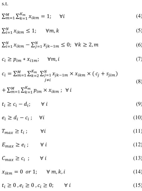
According to the above-mentioned assumptions and notations; the problem can be modelled by:
Min 𝑍1= 𝑇𝑚𝑎𝑥 (1)
Min 𝑍2= 𝐸𝑚𝑎𝑥 (2)
s.t.
∑𝑀𝑚=1∑𝐾𝑘=1𝑚 𝑥𝑖𝑘𝑚= 1; ∀𝑖 (4)
∑𝑁𝑖=1𝑥𝑖𝑘𝑚≤ 1; ∀𝑚, 𝑘 (5)
∑𝑁𝑖=1𝑥𝑖𝑘𝑚− ∑𝑁𝑗=1𝑥𝑗𝑘−1𝑚≤ 0; ∀𝑘 ≥ 2, 𝑚 (6)
𝑐𝑖≥ 𝑝𝑖𝑚∗ 𝑥𝑖1𝑚; ∀𝑚, 𝑖 (7)
𝑐𝑖= ∑ ∑ ∑𝑁𝑗=1𝑥𝑗𝑘−1𝑚× 𝑥𝑖𝑘𝑚× ( 𝑗≠𝑖
𝐾𝑚
𝑘=2 𝑀
𝑚=1 𝑐𝑗+ 𝑠𝑗𝑖𝑚)
+ ∑𝑀𝑚=1∑𝐾𝑘=1𝑚 𝑝𝑖𝑚× 𝑥𝑖𝑘𝑚 ; ∀𝑖
(8)
𝑡𝑖≥ 𝑐𝑖− 𝑑𝑖; ∀ 𝑖 (9)
𝑒𝑖≥ 𝑑𝑖− 𝑐𝑖 ; ∀𝑖 (10)
𝑇𝑚𝑎𝑥≥ 𝑡𝑖 ; ∀𝑖 (11)
𝐸𝑚𝑎𝑥≥ 𝑒𝑖 ; ∀ 𝑖 (12)
𝐶𝑚𝑎𝑥≥ 𝑐𝑖 ; ∀ 𝑖 (13)
𝑥𝑖𝑘𝑚= 0 𝑜𝑟 1; ∀ 𝑚, 𝑘, 𝑖 (14)
𝑡𝑖≥ 0 , 𝑒𝑖≥ 0 , 𝑐𝑖≥ 0; ∀ 𝑖 (15)
This model minimizes the maximum tardiness, maximum earliness and makespan stated by objective functions (1) to (3), respectively. Constraint (4) states that each job is assigned to exactly one position on one machine. Constraint (5) guarantees that assignment of at most one job to each position on each machine. Constraint (6) ensures that until one position on a machine is empty, jobs are not assigned to subsequent positions and jobs assigned to empty positions on each machines, respectively. Constraints (7) and (8) together ensure that only after starting the process by machine, no idle time could be inserted into the schedule, and no job preemption is allowed and should calculate the completion time of jobs. Constraint (9) is the definition
of the tardiness of jobs. Constraint (10) is the definition of the earliness of jobs. Constraint (11) defines the maximum tardiness. Constraint (12) defines the maximum earliness. Constraint (13) defines the maximum completion time. Constraints (14) and (15) define the type of decision variable.
3. SOLUTION ALGORITHM
A solution representation in HMOTLBO and a chromosome representation in NSGA-II is an array consisting of 𝑁 + 𝑀 − 1 real values between (0, 1).
Coding: An array consisting of 𝑁 + 𝑀 − 1real values
between (0, 1)
Decoding: Like a random key genetic algorithm
(RKGA), values sorted in a descending order then according to the position of each value in the main representation, an integer between 1 to 𝑁 + 𝑀 − 1do it. These are integer numbers as the coding scheme for a multi-machines scheduling problem. The integer number representation all possible permutation of 𝑁
jobs and 𝑀 − 1 machines. Numbers that are smaller than and equal 𝑁 represent jobs and numbers that are larger than 𝑁 represent machines. For example, number
𝑁 + 1 is 𝑀𝐴𝐶𝐻𝐼𝑁𝐸1, 𝑁 + 2 is 𝑀𝐴𝐶𝐻𝐼𝑁𝐸2 and
similarity 𝑁 + 𝑀 − 1 is 𝑀𝐴𝐶𝐻𝐼𝑁𝐸𝑀−1 and numbers
prior to them are jobs allocated to them. Finally, for numbers Finally, numbers with smaller than and equal to N are assigned to 𝑀𝐴𝐶𝐻𝐼𝑁𝐸𝑀. Following is a simple
example with nine jobs and three machines according Figure 1.
3. 1. Initial Population For two proposed
meta-heuristic algorithms, we produce solutions (learners)/ chromosomes to the number of the population size then compute objective functions according to Equations (11) to (13). For example, in the problem with nine jobs, three machines and population size 3, a sample of the population is shown in Table 1.
1. Producing 11 (3+9-1) real random in (0,1) and put them into the boxes:
1 2 3 4 5 6 7 8 9 10 11
0.905 0.127 0.913 0.964 0.097 0.278 0.546 0.957 0.970 0.157 0.632
2. Sorting real numbers in descending order
9 4 8 3 1 11 7 6 10 2 5
0.970 0.964 0.957 0.913 0.905 0.632 0.546 0.278 0.157 0.127 0.097
3. Decoding procedure
𝑀𝐴𝐶𝐻𝐼𝑁𝐸1 7,6
𝑀𝐴𝐶𝐻𝐼𝑁𝐸2: 9,4,8,3,1
𝑀𝐴𝐶𝐻𝐼𝑁𝐸3: 2,5
TABLE 1. Problem with 9 jobs, 3 machines and population size 3
𝑇𝑚𝑎𝑥 𝐸𝑚𝑎𝑥 𝐶𝑚𝑎𝑥
𝐿1 0.498 0.945 0.340 0.585 0.223 0.751 0.255 0.506 0.699 0.890 0.959 127 6 137
Population= 𝐿2 0.547 0.138 0.149 0.257 0.840 0.254 0.814 0.243 0.929 0.350 0.196 36 11 46
𝐿3 0.251 0.616 0.473 0.351 0.830 0.585 0.549 0.917 0.285 0.757 0.753 146 0 156
3. 2. Teaching–learning Based Optimization
Roa et al. [19] proposed a teaching-learning based optimization (TLBO) algorithm. This algorithm is based on learning a group of learners of a teacher in a class, and this group is considered as population. The teacher in each population is considered as the best learner. The learning process in this algorithm includes two stages, the first one is named teacher stage and the second the learner stage as explained hereunder:
3. 2. 1. Teacher Stage In this stage, the learners’
level of knowledge in iteration t(𝑥𝑖,𝑡)transfers by using
𝐷𝑀𝑡, i.e., difference between the teacher 𝑥𝑇,𝑡 and mean
result of learners 𝑀𝑡. Updated learner (𝑥𝑖,𝑡′ ) is
considered as follows:
𝑥𝑖,𝑡′ = 𝑥𝑖,𝑡+ 𝐷𝑀𝑡 (16)
where, 𝐷𝑀𝑡= 𝑟𝑡(𝑥𝑇,𝑡− 𝑇𝐹𝑀𝑡) (17)
TF is the teaching factor [19] and 𝑟𝑡is the random
number in the range [0, 1]. The detailed implementation for our problem is given as follows:
3. 2. 1. 1. Select Teacher In each iteration, the
teacher is considered to be the best learner, so form the
fronts and rank population using fast non-dominated sorting and compute the crowding distance [20]. Teacher selection based on select the solution with the lowest rank and in case of equality ranks, the solution with greater crowded distances is considered. The grade of the teacher is usually higher than the grade of the learner. Therefore, after selecting the best learner as the teacher by using hill-climbing search, the grade of the selected learner is increased and considered as teacher.
For example, learners’ ranks of the above example are (1,1,1), Because of Equal ranks, we compute the crowding distances as (3, ∞, ∞). According to computed crowding distances, learner 2 or learner 3 is considered as teacher. We select learner 2 as a teacher, then using hill climbing search, the selected teacher is improved (Table 2).
3. 2. 1. 2. Mean Result of Learners, 𝐌𝐭 For
obtaining the mean result of learners, calculate the mean of population columns (Table 2).
3. 2. 1. 3. 𝐃𝐌𝐭 The difference between the teacher
and the mean result at iteration t is computed using Equation (17).
For the above example, suppose that TF=1 and 𝑟𝑡= 0.8
(Table 2).
TABLE 2. Teacher stage
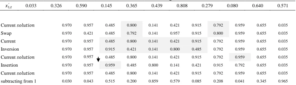
TABLE 3. Learner stage
Teacher 0.547 0.138 0.149 0.257 0.840 0.254 0.814 0.243 0.929 0.350 0.196
Mt 0.432 0.566 0.321 0.398 0.631 0.530 0.539 0.555 0.638 0.666 0.636
DMt 0.092 -0.342 -0.138 -0.113 0.167 -0.221 0.220 -0.250 0.233 -0.253 -0.352
x1,t′ 0.590 0.603 0.202 0.472 0.390 0.530 0.475 0.256 0.932 0.637 0.607
𝑥1,𝑡′ 0.033 0.326 0.590 0.145 0.365 0.439 0.808 0.279 0.080 0.640 0.571
Current 𝑠𝑜𝑙𝑢𝑡𝑖𝑜𝑛 0.970 0.957 0.485 0.800 0.141 0.421 0.915 0.792 0.959 0.655 0.035
Swap 0.970 0.421 0.485 0.792 0.141 0.957 0.915 0.800 0.959 0.655 0.035
Current 0.970 0.957 0.485 0.800 0.141 0.421 0.915 0.792 0.959 0.655 0.035
Inversion 0.970 0.957 0.915 0.421 0.141 0.800 0.485 0.792 0.959 0.655 0.035
Current 𝑠𝑜𝑙𝑢𝑡𝑖𝑜𝑛 0.970 0.957 0.485 0.800 0.141 0.421 0.915 0.792 0.959 0.655 0.035
Insertion 0.970 0.957 0.959 0.485 0.800 0.141 0.421 0.915 0.792 0.655 0.035
Current 𝑠𝑜𝑙𝑢𝑡𝑖𝑜𝑛 0.970 0.957 0.485 0.800 0.141 0.421 0.915 0.792 0.959 0.655 0.035
subtracting from 1 0.030 0.043 0.515 0.200 0.859 0.579 0.085 0.208 0.041 0.345 0.965
3. 2. 1. 4. Update the Learners Each learner in population is updated by using Equation (16). If the updated number is negative, it is converted to positive, and if the obtained number is greater than 1, let (obtained number-1) instead of it. For the above example, for learner 1(𝑥1,𝑡), updated form is 𝑥1,𝑡′ (Table
2):
3. 2. 1. 5. Acceptance Updated Learner If𝑥𝑖,𝑡′
dominates𝑥𝑖,𝑡, then replaced𝑥𝑖,𝑡 by 𝑥𝑖,𝑡′ . This work done
with Definition 1.
Definition 1. 𝑥𝑖 dominates 𝑥𝑗 if 𝑓(𝑥𝑖) ≤ 𝑓(𝑥𝑗) for all
objective functions and 𝑓(𝑥𝑖) < 𝑓(𝑥𝑗) for at least one
of objective functions [21].
For the above example, objective functions
𝑥1,𝑡 and 𝑥1,𝑡′ are (127 6 137) and (163 3 169)
respectively; therefore, 𝑥1,𝑡′ dose not dominate 𝑥1,𝑡,
and𝑥1,𝑡cannot be replaced by 𝑥1,𝑡′ .
3. 2. 2. Learner Stage In this stage, the fronts are
first formed and the population obtained from the teacher stage using fast non-dominated sorting is ranked as well, and the crowding distance is computed [20]. Then, the following steps in iteration t are carried out:
If 𝑟𝑎𝑛𝑘(𝑥𝑖,𝑡) < 𝑟𝑎𝑛𝑘(𝑥𝑗,𝑡) (if 𝑟𝑎𝑛𝑘(𝑥𝑖,𝑡) = 𝑟𝑎𝑛𝑘(𝑥𝑗,𝑡), then
if crowding distance (𝑥𝑖,𝑡)> crowding distance(𝑥𝑗,𝑡)), then
𝑥𝑖,𝑡′ = 𝑥𝑖,𝑡+ 𝑟𝑡(𝑥𝑖,𝑡− 𝑥𝑗,𝑡) 𝑟𝑡∈ (0,1) (19)
Step 1. For learner 𝑥𝑖,𝑡, randomly select another learner
If 𝑟𝑎𝑛𝑘(𝑥𝑗,𝑡) < 𝑟𝑎𝑛𝑘(𝑥𝑖,𝑡) (if 𝑟𝑎𝑛𝑘(𝑥𝑗,𝑡) = 𝑟𝑎𝑛𝑘(𝑥𝑖,𝑡)
then-if crowding distance (𝑥𝑗,𝑡)> crowding distance(𝑥𝑖,𝑡)), then
𝑥𝑖,𝑡′ = 𝑥𝑖,𝑡+ 𝑟𝑡(𝑥𝑗,𝑡− 𝑥𝑖,𝑡) 𝑟𝑡∈ (0,1) (20)
𝑥𝑗,𝑡 (𝑖 ≠ 𝑗).
Step 2. Update learner 𝑥𝑖,𝑡 (𝑥𝑖,𝑡′ ) by using Equations
(19) or (20).
Step 3. If updated number is negative converted to
positive and if obtained number is greater than 1, let (obtained number-1) instead of it.
Step 4.If 𝑥𝑖,𝑡′ dominates 𝑥𝑖,𝑡 , then replace 𝑥𝑖,𝑡 by 𝑥𝑖,𝑡′ .
Step 5. To make sure learning is done at the end of
learner stage, if learner 𝑥𝑖,𝑡 is not replaced by 𝑥𝑖,𝑡′ using
hill-climbing search, a better learner is replaced instead of 𝑥𝑖,𝑡.
For the above example, suppose for learner 1 (𝑥1,𝑡),
learner 3 (𝑥3,𝑡) is selected. According to Equation (20)
and 𝑟𝑡 =0.4, learner 1 is updated as follows (Table 3):
𝑥1,𝑡′ = 𝑥1,𝑡+ 𝑟𝑡(𝑥3,𝑡− 𝑥1,𝑡) (21)
Objective functions 𝑥1,𝑡 and 𝑥1,𝑡′ are (127 6 137) and
(129 2 139), respectively. Therefore, 𝑥1,𝑡′ dose not
dominate 𝑥1,𝑡, and𝑥1,𝑡cannot be replaced by 𝑥1,𝑡′ and
with hill climbing search 𝑥1,𝑡 is improved and inserted
to replace it. Teacher and learner stages are repeated until the stopping criteria is met.
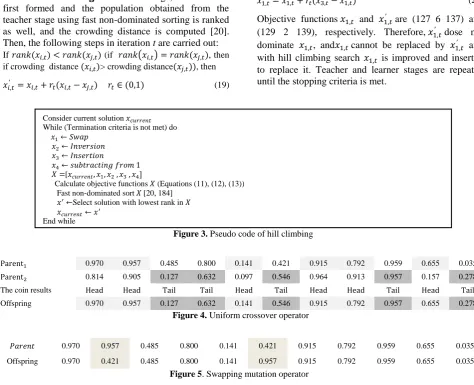
Figure 3. Pseudo code of hill climbing
𝑥1,𝑡′ = 𝑥1,𝑡+ 𝐷𝑀𝑡 (18)
Parent1 0.970 0.957 0.485 0.800 0.141 0.421 0.915 0.792 0.959 0.655 0.035
Parent2 0.814 0.905 0.127 0.632 0.097 0.546 0.964 0.913 0.957 0.157 0.278
The coin results Head Head Tail Tail Head Tail Head Head Tail Head Tail
Offspring 0.970 0.957 0.127 0.632 0.141 0.546 0.915 0.792 0.957 0.655 0.278
Figure 4. Uniform crossover operator
𝑃𝑎𝑟𝑒𝑛𝑡 0.970 0.957 0.485 0.800 0.141 0.421 0.915 0.792 0.959 0.655 0.035
Offspring 0.970 0.421 0.485 0.800 0.141 0.957 0.915 0.792 0.959 0.655 0.035
Figure 5. Swapping mutation operator 𝑥2← 𝐼𝑛𝑣𝑒𝑟𝑠𝑖𝑜𝑛
𝑥3← 𝐼𝑛𝑠𝑒𝑟𝑡𝑖𝑜𝑛
𝑥4← 𝑠𝑢𝑏𝑡𝑟𝑎𝑐𝑡𝑖𝑛𝑔 𝑓𝑟𝑜𝑚 1
𝑥𝑐𝑢𝑟𝑟𝑒𝑛𝑡← 𝑥′
Consider current solution 𝑥𝑐𝑢𝑟𝑟𝑒𝑛𝑡 While (Termination criteria is not met) do 𝑥1← 𝑆𝑤𝑎𝑝
𝑋 =[𝑥𝑐𝑢𝑟𝑟𝑒𝑛𝑡, 𝑥1, 𝑥2 , 𝑥3 , 𝑥4]
Calculate objective functions 𝑋 (Equations (11), (12), (13)) Fast non-dominated sort 𝑋 [20, 184]
𝑥′←Select solution with lowest rank in 𝑋
3. 3. Hill-climbing Search In this paper, we use four types of neighborhood structures that contain swap, inversion, insertion and subtracting from 1 [22] (Figure 2). A pseudo code of the proposed hill-climbing method is shown in Figure 3.
3. 4. NSGA-II The NSGA-II proposed in this paper
is described as follows: Parameters:
Pop: Population Npop: Population size
Pc: Percentage of the offspring population that completed with crossover operation
Pm: Percentage of the offspring population that completed with mutation operation
Npc: Numbers of offspring that created by crossover operation
Npm: Numbers of offspring that created by mutation operation
Tournament size: Number of individuals that are selected for tournament
Max-It: Maximum number of times to repeat the
algorithm (termination condition) Steps:
1. Create an initial population with Npop numbers by using Section 4 and calculate the value of objective functions𝐶𝑚𝑎𝑥, 𝑇𝑚𝑎𝑥and 𝐸𝑚𝑎𝑥(Equations (11) to
(13)).
2. Form the fronts and rank population using fast non dominated sorting and compute crowding distance [20].
3. Create population of offspring with Npop numbers that included Npc (Npop×Pc) individuals that are obtained from crossover operator (Figure 4), Npm (Npop×Pc) obtained from mutation operator (Figure 5) and reset individuals are selected from the parent population (all of selections for crossover operator, mutation operator and reset individual doing in the tournament size, using the non-dominated sorting and crowding distance individuals in the parent population).
4. Combine the parent population and offspring population and create the population with 2×Npop, then compute the non-dominated sorting and crowding distance of individual of the current population and for creating a new population with Npop individual use the method offered by Deb et al. [20].
5. Repeat Steps 1 to 4 until Max-It is occurred.
3. 5. ε-constraint Method In this method, one of
the objective functions is placed as objective function and optimized. The other objective functions are transferred into constraints as follows:
Min 𝑓𝑗(𝑥) (22)
s.t.
𝑓ℎ(𝑥) ≤ 𝜀ℎ; ℎ = 1, … , 𝑚, ℎ ≠ 𝑗,
𝑓ℎ𝑚𝑖𝑛≤ 𝜀ℎ≤ 𝑓ℎ𝑚𝑎𝑥
(23)
𝑥 ∈ 𝑆 (24)
where 𝑗 ∈ {1, … , 𝑚} and 𝜀ℎ is upper bounds for the
objective h (ℎ ≠ 𝑗). VariousPareto solutions can be found by changing the value of 𝜀ℎ. We can let 𝑓ℎ𝑚𝑖𝑛=
𝑓ℎ∗ and 𝑓ℎ𝑚𝑎𝑥 = 𝑓ℎ𝑛𝑎𝑑𝑖𝑟 by using payoff matrix [21]. We
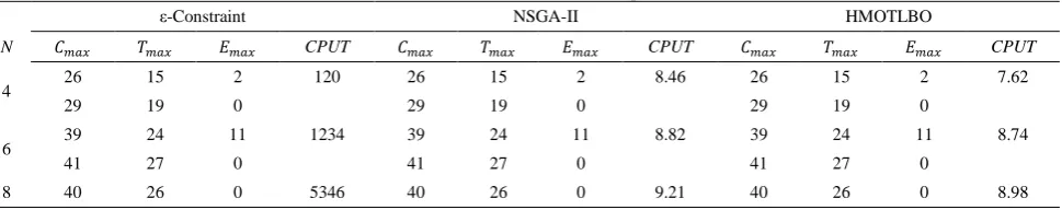
consider three sample problems in small sizes with 8, 6 and 4 jobs and 2 machines. These problems are solved with Lingo 8.0 and their results are shown in Table 10, in which the results of two proposed algorithms for the same problems are presented as well.
4. COMPUTATIONAL RESULTS
In order to test the effectiveness of the NSGA-II and HMOTLBO, we solve several test problems, (e.g., Naderi-Beni et al. [23]), and then compare their performances with a number of different metrics. The proposed meta-heuristics are coded in MATLAB R2016a software.
4. 1. Test Problem Instances Computational
results given in [23] are conducted in medium and large-sized problems according to Tables 4 and 5. The processing times (𝑝𝑖𝑚) are integers and are generated
from a uniform distribution of U(1, 20), the due dates (𝑑𝑖) are uniformly distributed in the interval [𝑃 (1 − 𝑡 − 𝑟
2) , 𝑃 (1 − 𝑡 + 𝑟
2)], where 𝑃 =
∑𝑁𝑖=1∑𝑀𝑗=1𝑝𝑖𝑗
2𝑀 , t =0.8 , r
=0.2 and the setup times are integers and are generated from a uniform distribution of U(1, 20).
4. 2. Evolution Metric Quality of the
non-dominated solutions obtained from the proposed meta-heuristic algorithms is used to compare these algorithms. In this paper, three metrics (i.e., N-metric, R-metric and S-metric) are used [24].
4. 3. Parameter Tuning The quality of the
our results, best combinations of parameters for medium and large problems are showed in Table 7.
For tuning the parameters of HMOTLBO, the levels of these parameters are shown in Table 8. For the given
TABLE 4. Medium-sized problems.
M N M N M N M N
3 10 4 15 5 20 6 25
3 20 4 30 5 40 6 50
3 30 4 45 5 60 6 75
3 40 4 60 5 80 6 90
TABLE 5. Large-sized problems.
M N M N M N M N
7 30 8 35 9 20 10 45
7 60 8 70 9 40 10 90
7 90 8 105 9 60 10 135
7 120 8 140 9 80 10 180
TABLE 6. The levels of NSGA-II parameters
Levels
Parameters Lower Upper
MaxIt 10 90
Npop 50 210
Pc 0.1 0.9
Pm 0.02 0.1
TABLE 7. Best combinations of NSGA-II parameters
Parameters
Max-It Npop Pc Pm
Value
M 60 150 0.6 0.07
L 50 210 0.5 0.06
parameters, the RMS designs 20 experiments that contain six central and 14 axial points. According to the results, the best combinations of parameters for medium and large-sized problems are shown in Table 9.
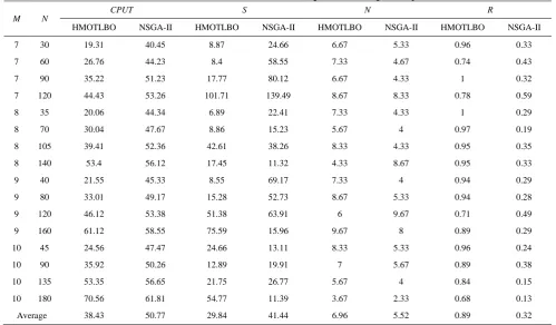
4. 4. Evaluating Results Each proposed algorithm
is run 3 times and each time includes 10 runs in 32 test problems including 16 medium problems and 16 large problems (Tables 4 and 5).The average results of 3 times are shown in Tables 11 and 12. The results of small problems are given in Table 10 that shows for
small problems (N=4, 6, 8 and M=2), HMOTLBO and NSGA-II produce Pareto-optimal solutions similar to the ε-constraint method, although CPUT is reduced significantly. Tables 11 and 12 show that the HMOTLBO is better than the NSGA-II in terms of different metrics for medium and large-sized problems. The amount of changing the solving times in NSGA-II is less than HMOTLBO. Solving times in NASGA-II versus HMOTLBO has substantially reduced in larger size problems. Nvalues in both algorithms are relatively close; however, Rvalues are different. The results show that NSGA-II produces lots of Pareto solutions, but dominated by a few Pareto solutions produced by HMOTLBO.
TABLE 8. Levels of HMOTLBO parameters
Levels
Parameters Lower Upper
Max-It 5 25
Npop 10 30
TF 1 2
TABLE 9. Best combinations of HMOTLBO parameters
Parameters
MaxIt Npop TF
M 15 30 1
L 15 25 1.25
TABLE 10. Results for small-sized problem
N
ε-Constraint NSGA-II HMOTLBO
𝐶𝑚𝑎𝑥 𝑇𝑚𝑎𝑥 𝐸𝑚𝑎𝑥 CPUT 𝐶𝑚𝑎𝑥 𝑇𝑚𝑎𝑥 𝐸𝑚𝑎𝑥 CPUT 𝐶𝑚𝑎𝑥 𝑇𝑚𝑎𝑥 𝐸𝑚𝑎𝑥 CPUT
4 26 15 2 120 26 15 2 8.46 26 15 2 7.62
29 19 0 29 19 0 29 19 0
6 39 24 11 1234 39 24 11 8.82 39 24 11 8.74
41 27 0 41 27 0 41 27 0
TABLE 11. Results of NSGA-II and HMOTLBO algorithms for medium-sized problems
M N
CPUT S N R
HMOTLBO NSGA-II HMOTLBO NSGA-II HMOTLBO NSGA-II MOTLBOH NSGA-II
3 10 15.17 23.57 3.11 1.77 3 3 0.77 0.83
3 20 16.64 24.24 4.12 4.97 4.67 3.33 0.96 0.6
3 30 19.36 24.81 12.45 77.85 6 6.67 0.84 0.57
3 40 22.18 25.40 156.91 18.75 5.33 9.67 0.69 0.76
4 15 16.52 24.32 2.57 2.48 4 3.33 1 0.4
4 30 20.33 25.54 25.88 94.49 7.33 4.67 1 0.29
4 45 24.15 25.87 18.96 45.40 6.67 5.67 0.87 0.49
4 60 27.09 26.79 22 142.81 6.67 8 0.81 0.59
5 20 18.90 24.71 14.70 7.33 7.67 1.67 0.95 0.16
5 40 23.38 26.48 4.07 127.91 6.33 3.67 0.97 0.31
5 60 29.64 27.40 18.72 29.22 9.33 4.33 0.85 0.38
5 80 35.95 29.46 38.25 7.15 6 9.67 0.96 0.53
6 25 21.56 26.64 7.55 25.79 8 5.33 1 0.34
6 50 26.12 26.78 30.86 23.40 9 6.67 0.86 0.44
6 75 34.32 28.55 111.63 59.39 8.33 6 0.81 0.47
6 90 42.14 30.72 52.92 32.51 4.67 10.33 0.68 0.68
Average 24.59 26.33 32.79 43.83 6.44 5.75 0.88 0.49
TABLE 12. Results of NSGAII and HMOTLBO algorithms for large-sized problems
M N
CPUT S N R
HMOTLBO NSGA-II HMOTLBO NSGA-II HMOTLBO NSGA-II HMOTLBO NSGA-II
7 30 19.31 40.45 8.87 24.66 6.67 5.33 0.96 0.33
7 60 26.76 44.23 8.4 58.55 7.33 4.67 0.74 0.43
7 90 35.22 51.23 17.77 80.12 6.67 4.33 1 0.32
7 120 44.43 53.26 101.71 139.49 8.67 8.33 0.78 0.59
8 35 20.06 44.34 6.89 22.41 7.33 4.33 1 0.29
8 70 30.04 47.67 8.86 15.23 5.67 4 0.97 0.19
8 105 39.41 52.36 42.61 38.26 8.33 4.33 0.95 0.35
8 140 53.4 56.12 17.45 11.32 4.33 8.67 0.95 0.33
9 40 21.55 45.33 8.55 69.17 7.33 4 0.94 0.29
9 80 33.01 49.17 15.28 52.73 8.67 5.33 0.94 0.28
9 120 46.12 53.38 51.38 63.91 6 9.67 0.71 0.49
9 160 61.12 58.55 75.59 15.96 9.67 8 0.89 0.29
10 45 24.56 47.47 24.66 13.11 8.33 5.33 0.96 0.24
10 90 35.92 50.26 12.89 19.91 7 5.67 0.89 0.38
10 135 53.35 56.65 21.75 26.77 5.67 4 0.84 0.15
10 180 70.56 61.81 54.77 11.39 3.67 2.33 0.68 0.13
5. CONCLUSION AND FUTURE RESEARCH
This paper has studied a multi-objective unrelated parallel machines scheduling problem in order to minimize the makespan, maximum tardiness and maximum earliness of jobs, in which sequence-dependent setup times are machine-dependent processing times have been considered. Additionally, a multi- objective mixed-integer linear programming (MILP) model has been formulated, and then solved by the ε-constraint method for small-sized problems. The results have been compared with the results obtained by the proposed meta-heuristic algorithms. Furthermore, an effective hybrid multi-objective teaching–learning based optimization (HMOTLBO) has been proposed. Its performance has been compared with a non-dominated sorting genetic algorithm (NSGA-II) on a number of test problems generated at random. The related results have shown that the proposed HMOTLBO is relatively better than the NSGA-II.
In this study, we have considered real conditions in an industrial environment. Of course, there are other conditions that help us to improve our research, such as taking into account pre-emption, precedence constrains and machine failures. Also, one can use other meta-heuristic algorithms and compare the results with our results.
6. REFERENCES
1. Chang, P. C. and Chen, S.-H., "Integrating dominance properties with genetic algorithms for parallel machine scheduling problems with setup times", Applied Soft Computing, Vol. 11, No. 1, (2011), 1263-1274.
2. Tavakkoli-Moghaddam, R. and Mehdizadeh, E., "A new ILP model for identical parallel-machine scheduling with family setup times minimizing the total weighted flow time by a genetic algorithm", International Journal of Engineering Transactions A Basics, Vol. 20, No. 2, (2007), 183-194.
3. Tavakkoli-Moghaddam, R., Taheri, F. and Bazzazi, M., "Multi-objective unrelated parallel machines scheduling with sequence-dependent setup times and precedence constraints",
International Journal of Engineering, Transactions A: Basics, Vol. 21, No. 3, (2008), 269-278.
4. Tavakkoli-Moghaddam, R. and Aramon-Bajestani, M., "A novel b and b algorithm for a unrelated parallel machine scheduling problem to minimize the total weighted tardiness", International Journal of Engineering, Vol. 22, No. 3, (2009), 269-286. 5. Torabi, S. A., Sahebjamnia, N., Mansouri, S. A. and Bajestani,
M. A., "A particle swarm optimization for a fuzzy multi-objective unrelated parallel machines scheduling problem",
Applied Soft Computing, Vol. 13, No. 12, (2013), 4750-4762.
6. Lin, S.-W. and Ying, K.-C., "Abc-based manufacturing scheduling for unrelated parallel machines with machine-dependent and job sequence-machine-dependent setup times", Computers & Operations Research, Vol. 51, (2014), 172-181.
7. Rodriguez, F. J., Lozano, M., Blum, C. and GarciA-MartiNez, C., "An iterated greedy algorithm for the large-scale unrelated
parallel machines scheduling problem", Computers & Operations Research, Vol. 40, No. 7, (2013), 1829-1841.
8. Bozorgirad, M. A. and Logendran, R., "Sequence-dependent group scheduling problem on unrelated-parallel machines",
Expert Systems with Applications, Vol. 39, No. 10, (2012), 9021-9030.
9. Lin, Y.-K., Pfund, M. E. and Fowler, J. W., "Heuristics for minimizing regular performance measures in unrelated parallel machine scheduling problems", Computers & Operations Research, Vol. 38, No. 6, (2011), 901-916.
10. Nogueira, J. P., Arroyo, J. E. C., Villadiego, H. M. M. and Goncalves, L. B., "Hybrid grasp heuristics to solve an unrelated parallel machine scheduling problem with earliness and tardiness penalties", Electronic Notes in Theoretical Computer Science, Vol. 302, (2014), 53-72.
11. Gharehgozli, A., Tavakkoli-Moghaddam, R. and Zaerpour, N., "A fuzzy-mixed-integer goal programming model for a parallel-machine scheduling problem with sequence-dependent setup times and release dates", Robotics and Computer-Integrated Manufacturing, Vol. 25, No. 4, (2009), 853-859.
12. Kayvanfar, V., Komaki, G. M., Aalaei, A. and Zandieh, M., "Minimizing total tardiness and earliness on unrelated parallel machines with controllable processing times", Computers & Operations Research, Vol. 41, (2014), 31-43.
13. Tavakkoli-Moghaddam, R., Taheri, F., Bazzazi, M., Izadi, M. and Sassani, F., "Design of a genetic algorithm for bi-objective unrelated parallel machines scheduling with sequence-dependent setup times and precedence constraints", Computers & Operations Research, Vol. 36, No. 12, (2009), 3224-3230. 14. Gao, J., "A novel artificial immune system for solving
multiobjective scheduling problems subject to special process constraint", Computers & Industrial Engineering, Vol. 58, No. 4, (2010), 602-609.
15. Chyu, C.-C. and Chang, W.-S., "A pareto evolutionary algorithm approach to bi-objective unrelated parallel machine scheduling problems", The International Journal of Advanced Manufacturing Technology, Vol. 49, No. 5-8, (2010), 697-708.
16. Lin, Y.-K. and Lin, H.-C., "Bicriteria scheduling problem for unrelated parallel machines with release dates", Computers & Operations Research, Vol. 64, (2015), 28-39.
17. Mir, M. S. S. and Rezaeian, J., "A robust hybrid approach based on particle swarm optimization and genetic algorithm to minimize the total machine load on unrelated parallel machines",
Applied Soft Computing, Vol. 41, (2016), 488-504.
18. Joo, C. M. and Kim, B. S., "Hybrid genetic algorithms with dispatching rules for unrelated parallel machine scheduling with setup time and production availability", Computers & Industrial Engineering, Vol. 85, (2015), 102-109.
19. Rao, R. V., Savsani, V. J. and Vakharia, D., "Teaching–learning-based optimization: A novel method for constrained mechanical design optimization problems", Computer-Aided Design, Vol. 43, No. 3, (2011), 303-315.
20. Deb, K., Pratap, A., Agarwal, S. and Meyarivan, T., "A fast and elitist multiobjective genetic algorithm: NSGA-ii", IEEE Transactions on Evolutionary Computation, Vol. 6, No. 2, (2002), 182-197.
21. Deb, K. and Miettinen, K., "Multiobjective optimization: Interactive and evolutionary approaches, Springer Science & Business Media, Vol. 5252, (2008).
22. Soni, N. and Kumar, T., "Study of various mutation operators in genetic algorithms", International Journal of Computer Science and Information Technologies (IJCSIT), Vol. 5, No. 3, (2014), 4519-4521.
a parallel machine scheduling problem with machine eligibility restrictions and sequence-dependent setup times", International Journal of Production Research, Vol. 52, No. 19, (2014), 5799-5822.
24. Han, Y.-Y., Gong, D.-w., Sun, X.-Y. and Pan, Q.-K., "An
improved NSGA-ii algorithm for multi-objective lot-streaming flow shop scheduling problem", International Journal of Production Research, Vol. 52, No. 8, (2014), 2211-2231.
25. Montgomery, D. C., "Design and analysis of experiments, John Wiley & Sons, (2008).
Solving a New Multi-objective Unrelated Parallel Machines Scheduling Problem by
Hybrid Teaching-learning Based Optimization
A. Sadatia, R. Tavakkoli-Moghaddamb, B. Naderic, M. Mohammadic
a Department of Industrial Engineering, Science and Research Branch, Islamic Azad University, Tehran, Iran b School of Industrial Engineering, South Tehran Brach, Islamic Azad University, Tehran, Iran
c Department of Industrial Engineering, Faculty of Engineering, Kharazmi University, Tehran, Iran P A P E R I N F O
Paper history:
Received 22 December 2016
Received in revised form 19 January 2017 Accepted 22 January 2017
Keywords:
Teaching–learning Based Optimization Unrelated Parallel Machines Makespan Tardiness Earliness ديكچ ه ا رد ی ن ،هلاقم هلأسم نامز دنب ی ی ک هعومجم زا اهراک ی غ ی ر ور هتسباو ی شام ی ن اه ی زاوم ی غ ی ر ی ناسک هب روظنم مک ی هن ندرک بی ش ی هن نامز مکت ی ل اهراک لوط( همانرب نامز دنب ی ،) بی ش ی هن د ی درکر و ب ی ش ی هن درکدوز دروم هعلاطم رارق م ی گ ی در . اهراک اراد ی اهدعوم ی وحت ی ل غ ی ر ی ،ناسک نامز اه ی هار زادنا ی لاوت هب هتسباو ی
نامز و اه ی شام هب هتسباو شزادرپ ی ن م ی .دنشاب ی ک لدم همانرب ر ی ز ی طخ ی ددع حص ی ح طلتخم هفدهدنچ دروم هجوت رارق م ی گ ی در اب لئاسم رد هک شور اب کچوک هزادنا
ودحم ی ت -سپا ی نول لح دروم هدش تسا . سپس ، اتن ی ج اتن اب ی ج لصاح زا روگلا ی مت اه ی راکتباارف ی ب ی نا هدش اقم ی هس م ی .دنوش ی ک روگلا ی مت هب ی هن زاس ی فلت هفدهدنچ ی ق ی شزومآ ساسا رب -ی گدا ی ر ی (HMOTLBO) پی داهنش م ی دوش اراک و یی ا ی ن روگلا ی مت پی داهنش ی اب روگلا ی مت نژ ی کت بترم هدش غ ی بولغمر (NSGA-II) ور ی دادعت ی فداصت تروص هب هک هنومن لئاسم زا ی لوت ی د هدش اقم ،دنا ی هس م ی اتن .دنوش ی ج ناشن م ی روگلا هک دهد ی مت پ ی داهنش ی HMOTLBO هب تبسن NSGA-II اتن ی ج رتهب ی ار م هئارا ی .دهد