Deterministic and Metaheuristic Solutions for Closed-loop Supply Chains with Continuous Price Decrease

Please cite this article as: H.R. Kamali, A. Sadegheih, M.A. Vahdat-Zad, H. Khademi-Zare, Deterministic and Metaheuristic Solutions for Closed-loop Supply Chains with Continuous Price Decrease, International Journal of Engineering (IJE), TRANSACTIONS C: Aspects Vol. 27, No. 12, (December 2014) 1897-1906

International Journal of Engineering

J o u r n a l H o m e p a g e : w w w . i j e . i r

Deterministic and Metaheuristic Solutions for Closed-loop Supply Chains with

Continuous Price Decrease

H. R. Kamali*, A. Sadegheih, M. A. Vahdat-Zad, H. Khademi-Zare

Department of Industrial Engineering, University of Yazd, Yazd, Iran

P A P E R I N F O

Paper history:

Received 28 February 2014 Received in revised form 11 May 2014 Accepted 14 August 2014

Keywords:

Closed-loop Supply Chain Continuous Price Decrease NP-hard

Metaheuristic

A B S T R A C T

In a global economy, an efficient supply chain as the main core competency empowers enterprises to provide products or services at a right time in a right quantity, and at a low cost. This paper is to plan a single-product, multi-echelon, multi-period closed-loop supply chain for high-tech products (which have continuous price decrease). Ultimately, considering components ralated to procurement, production, distribution, recycling and disposal, the final decisions are made. To solve the mixed integer linear programming model for closed-loop supply chain network plan of the paper, four heuristics-based methods including genetic algorithm, particle swarm optimization, differential evolution, and artificial bee colony are proposed. Finally, the computational results of these four methods are compared with the solutions obtained by GAMS optimization software. The solution reveales that the artificial bee colony methodology works well in terms of quality of solutions.

doi: 10.5829/idosi.ije.2014.27.12c.13

1. INTRODUCTION1

Supply chain (SC) is a result of linking different operational parts in which suppliers lie at the beginning and customers at the end. A SC points to the flow of materials, information, cash, and services from raw material suppliers to workshops and warehouses and finally to customers. It includes processes and organizations that create products, information, and services and delivers them to consumers.

A closed-loop supply chain (CLSC) is a SC that has some extra parts for collecting returned products from customers, recycling and reusing them to produce new products. Nowadays, CLSC management is one of the topics discussed in the area of industrial management. It has been taken into consideration by industry owners for their vehement tendency to decrease costs, establish ever-increasing interaction among producers, suppliers

1_{*Corresponding Author’s Email: [email protected] (H. R.} Kamali)

and distributers at various levels, and create more and more SCs as well as CLSCs for different products.

The methods that have been used for SC or CLSC optimizing are also various. Analytical methods, such as branch and bound, present optimal solutions, but their performance highly declines by the increase in the dimensions of problems. Some other analytical methods are used only for certain problems in special conditions [1, 2]. Simulation of dynamic systems is a method that forecasts the behavior of a model by changing its parameters [3]. Heuristic methods provide approximate solutions to problems, and they usually have a simple structure and short running time [4]. Using metaheuristic algorithms is another way to optimize a SC or CLSC. These methods have a general structure and can be matched with different problems. They do not guarantee to make optimal solutions, but they usually find optimal or near optimal solutions. For example, some metaheuristic algorithms used for SC or CLSC optimization are genetic algorithm [5], differential evolution [6] and simulated annealing [7].

TABLE 1. Some recent studies done on CLSC planning

Batch delivery

Time duration considering

Dynamic demands

Multiple market

Cost (Ordering Holding Shortage)

Ref.

[9] [10]

n n OH [11]

n n H [12]

n H [13]

n n H [14]

n n n n OHS _Study This

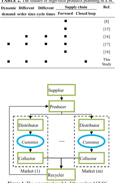
TABLE 2. The studies of high-tech products planning in a SC

Dynamic demand

Different order sizes

Different cycle times

Supply chaiu Ref. Forward Closed loop

n [8]

n [15]

n n n [16]

n n n n [17]

n [18]

n n n n _Study This

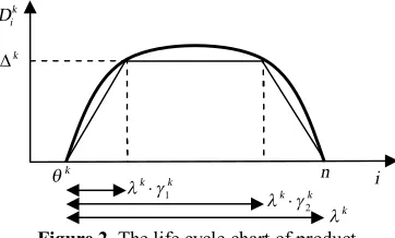
Figure 1. The conceptual model of the explored CLSC

High-tech products are the ones produced by advanced technology. They have a short life cycle and become obsolete very fast because the technology grows rapidly and an intense competition exists between industry owners. Thus, component costs and product sale prices decrease over time (continuous price decrease). For example, in some industries like computer and communication, the production costs and

sale prices decrease for one percent per week [8]. So, as a result of fast distribution of these products, a higher income is gained. Owing to this point and considering the transportation and delivery fixed costs and limited production rate, the production management and planning of high-tech products seems very necessary.

The novelty of this study can be considered in two contexts, 1) CLSC planning and 2) high-tech products planning. Planning of CLSCs is a topic that was taken into consideration by many researchers. This topic is very various because different conditions can be assumed for CLSCs, and each of the assumptions creates a new problem. Table 1 categorizes some recent studies done in this respect.

Regarding the research done, this study has investigated the following assumptions that have not been paid attention together in the previous studies.

1) Components and products are transported between the levels of the chain in batches.

2) The duration times of supplying, producing and transporting are considered in the model.

3) The demands in different periods can be different. 4) Ordering, holding and shortage costs are all taken

into consideration.

Furthermore, in this study, the limitations of shipment size and stores capacity are taken into account, which adds to the novelty of the study.

Also, some research has been done in the context of production and delivery planning for high-tech products (which have continuous price decrease). Some of these studies are in a single system, and some are in a SC. Table 2 categorizes the studies conducted in a SC. As it can be seen in Table 2, the present study is the first study that planned a CLSC for products with continuous price decrease.

The structure of the paper is as follows. Section 2 defines and describes the problem. Different parts of the model are presented in section 3. In section 4, the method for solving the problem is described. In section 5, a numerical example of the problem is offered and solved, and finally, section 6 presents the results.

2. STATEMENT OF THE PROBLEM

The examined problem is planning a multi-echelon CLSC. Figure 1 shows the corresponding conceptual model. It includes a supplier, a producer, some potential markets, and a recycler. Each potential market includes a distributor, a customer population, and a collector. At first, the components that are required for production are ordered by the supplier, and then they are shipped from the supplier to the producer. After production, the products are shipped to the distributor of active markets to be sold to their customers. Some of the used products are returned by the customers and are purchased by the

Supplier

Producer

Distributor

Recycler

Collector Distributor

Collector

Customer

Market (1)

….

Customer

collectors. Each collector disposes some of these returned products and shippes some of them to a recycler. The recycler does an operation on these returned products, recycles the recyclable parts, and ships them to the producer to be reused in production.

The components that any producer uses to produce the products can be divided into two groups. The components of the first group are obtained by recycling the returned products. They are obviously obtainable from the supplier, too. However, the components of the second group are obtainable only from the supplier rather than by recycling the returned products. The assumptions of the stated problem are as follows. 1) A single-product multi-echelon CLSC is examined. 2) There are some potential markets to sell products. 3) The time horizon is limited, which equals to the life

cycle of the problem.

4) The demand is deterministic and dynamic. 5) The rates of production and recycling are limited. 6) Confronting an inventory shortage is allowed. The

shortage is as a backlog, and its cost is time-dependent.

7) Setting up for production and recycling has fixed costs.

8) The production and recycling are gradual and continuous, but the batches of components and products are delivered immediately at the beginning of each period.

9) The objectives of planning are selecting active markets to cover and determine the values and times for ordering and shipping components and products to maximize the total profit.

10)The optimization method for the examined problem is considered as a centralized optimization with benefit sharing [11].

3. MODEL DESCRIPTION

The mathematical model of the stated problem is defined as a mixed integer linear programming (MILP) model whose parameters and variables are defined as follows (i: Index of time periods, k: Index of markets).

3. 1. Model’s Parameters and Variables The

parameters of the model are as follows. r: Studied time horizon

n: Number of time periods

m: Number of markets k

FC : Fixed cost of covering kth market k

BC : Shortage cost of each unit of the product in each time period by the distributor

SP: Setup cost for production by the producer SR: Setup cost for recycling by the recycler

GP: Processing cost per unit of the products by the producer

k

GS : Processing cost for destructing each unit of retuned product by the collector

GR: Processing cost per unit of the retuned products by

the recycler

MP: Capacity of production in each period by the producer

k

MG : Capacity of each shipment of products from the

producer to the distributor k

MH : Capacity of each shipment of returned products

from the collector to the recycler

MR: Capacity of recycling in each period by the recycler

TS: Required time for purchasing components by the supplier

TE: Required time for transporting components from the supplier to the producer

k

TG : Required time for transporting products from the

producer to the distributor k

TH : Required time for transporting returned products from the distributor to the recycler

TQ: Required time for transporting recycled first group components from the recycler to the producer

1

k

t : Return rate of the sold products in the first period

2

k

t : The increment value of the return rate of the sold products in the periods

k i

D : Demand of the products

k i

P : Sale price of the products

i

UA: Purchasing cost of each unit of the first group

components by the supplier

A

a : First parameter of purchasing unit cost of the first group components by the supplier

A

b : First parameter of purchasing unit cost of the first group components by the supplier

i

UB: Purchasing cost of each unit of the second group

components by the supplier B

a : First parameter of purchasing unit cost of the second group components by the supplier B

b : Second parameter of purchasing unit cost of the second group components by the supplier k

i

UI : Purchasing cost of each unit of the returned products by the collector

1

k

g : First parameter of the product demand

2

k

g : Second parameter of the product demand k

D : Third parameter of the product demand

RH: Rate of holding cost

RP: Ratio of purchasing cost for the returned products to their sale price

RR: Ratio of recycling rate to production rate

A

AS : Supplier’s expected profit for delivering each unit

B

AS : Supplier’s expected profit for delivering each unit

of the second group component

AP: Producer’s expected profit for delivering each unit of the product

k

AD : Expected profit of k_th market’s distributor for selling each unit of the product

The real and non-negative decision variables of the model are as follow.

i

XP: Quantity of production by the producer

k i

XG : Quantity of shipping the products from the producer to the distributor

k i

XH : Quantity of shipping the returned products from the collector

k i

XS : Quantity of disposing the returned products by the collector

i

XR: Quantity of recycling by the recycler

i

PI: Inventory level of the products for the producer

k i

S : Quantity of selling the products by the distributor k

i

DC : Quantity of the returned products to the collector

i

PP: Inventory level of the recycled first group

components for the recycler

Also, the binary variable _WMk is defined as follows: It is equal to 1 if k_th market is covered (be active); otherwise, it is equal to 0.

Other parameters and variables are as follows: VA,

VB, VE, VF, VDk, _VCk, _VR,

VQ, MA, MB, ME, MF, MQ

, HA, HB, HE, HF, HI, _HDk_{, HC}k, _HR, _HP,_FA, _FB, FE, FF, _FDk, _FR,

FQ,CA, CB, CE, CF, CI, _CDk, _CCk, CR, CQ, XA, XB , XE , XF , XQ , PI , PD , PC , PR

. Each of these parameters and variables has two letters that are described in below.

- For the first letter: F: fixed order cost, V: variable order cost for each unit, M: the capacity of the shipment, H: holding cost, C: warehouse capacity, X: quantity of purchasing and shipping, and P: inventory level.

- For the second letter: ,A B: first and second group purchased components by the supplier, ,E F: first and second group components of the producer, I : products of the producer, D: products of the distributor, C: returned products of the collector,

R: returned products of the recycler, and Q: recycled first group components of the recycler.

3. 2. Calculating Related Parameters The

parameters of purchasing cost of components, product’s sale price, purchasing cost of returned products, product’s demand, used product’s rate of return, unit holding cost, and recycling capacity depend on other parameters and result from them. These calculations are expressed at below. The range of indices are as

1,...,

i= n _and k=1,...,m.

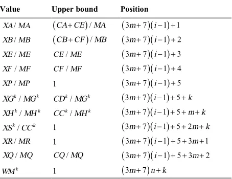
Figure 2. The life cycle chart of product

Because the product belongs to high-tech products group, it is supposed that the purchasing cost of components and, consequently, theproduct’s sale price and the purchasing cost of returned products decrease linearly. To calculate the decreasing cost of the first group components and the second group components, Equations (1) and (2) are used, respectively. Equation (3) calculates the product’s sale price. Also, the purchasing cost of the returned product is calculated by Equation (4).

( )

1

i A A

UA=a -b i- (1)

( 1)

i B B

UB =a -b i- (2)

k k

i i A i B

P =UA AS+ +UB+AS +GP AP AD+ + (3)

k k

i i

UI =P RP× (4)

The demand is considered as deterministic and dynamic, which follows the product’s life cycle [19]. Therefore, the curve of the product’s life cycle is estimated as a trapezoidal shape (Figure 2), and the demand is determined in its three parts by Equations (5) to (7). These calculations should be done for each market, separately.

The ratio of returned products to sold products in k_th

market after i _{period of their sale time is calculated by}

Equations (8) and (9). The unit holding cost of components and products is a fraction of inventory value that is calculated according to Equations (10) to (18). Also, the recycling capacity is calculated by Equation (19).

2

k _{TS TE TG}k

q = + + + (5)

1

k _n k

l = -q + (6)

(

)

( )

(

)

1 1 1 2 2 2 0, 1 , 1 , 1 , 1 k k k

k k k k

k k k

i _{k k k k k k k}

k

k k k

k k i i i D i n i i n q q

q q l g

l g

q l g q l g

q l g

l g

ì _< ï

ï D - +

ï _{£ £ + ×}

ï _{× +} ï

= í

D + × £ £ + × ï

ï D - + ï + × £ £ ï -ï î ₍₇₎ 1 k k l g×

2 k k l g× _k

0 0 k

w = (8)

( )

(

)

1

1 2

0

1 1 i

k k k k

i j

j i

w t t -w

=

æ ö

= + - ç - ÷

è

å

ø (9)

i i

HA RH UA n r

= (10)

i i

HB RH UB n r

= ₍₁₁₎

i i

HE RH UA n r

= (12)

i i

HF RH UB n r

= (13)

( )

i i i

HI RH UA UB GP n

r

= + + (14)

( )

k

i i i

HD RH UA UB GP n

r

= + + (15)

k k

i i

HC RH UI n r = (16) 1 m k i i k HR RH UI

m n r

= =

× å (17)

1 1 m

k

i i

k

HP RH UI GR n m

r =

æ ö

= _ç + _÷

è å ø (18)

MR MP RR= × (19)

3. 3. Relationship Among the Model’s Variables

Figure 3 shows the relationship among the variables of the surveyed model.

3. 4. NP-hardness of the Problem In the

considered problem, the production rate is limited, and each potential market has a deterministic demand. The purpose is to select some active markets among potential ones to maximize the total earned profit. This problem is like Knapsack problem. Therefore, it can be concluded that it is NP-hard.

4. SOLUTION METHODOLOGY

To plan the explored CLSC problem, the time horizon is divided into some equal periods, and planning is done for them. The more the number of divisions or periods, the closer the planning to reality, the more the dimensions of the problem, and the more the amount of the solving time needed. This is especially true in NP-hard problems. When analytic methods such as branch and bound method (for solving MILP model) are used, an increase of the problem dimensions leads to a drastic increase of the solving time. Thus, in the case of these problems, metaheuristic algorithms should be used to make a near optimal solution.

The model considered in this study is a large model. This can be understood by considering a small problem

that has seven periods and ten potential markets but as many as 269 variables (i.e. dimensions) in each solution, which is a large number. This is why optimizing such a problem, even with metaheuristic algorithms, is difficult, and certain modifications should be done in the solving methods to promote their efficiency. These modifications are applied in creating a primary population as below.

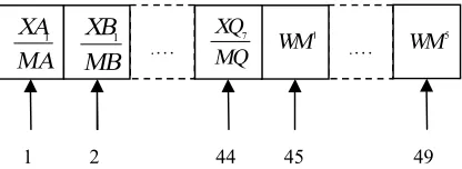
4. 1. Solution Structure and Evaluation Method

Each solution in the explored problem is like a string of real numbers resulting from the variables of the problem. If n is the number of time periods and m is the number of potential markets, the length of this string is equal to

(

3m+7

)

n m+ . To convert the problem variables to a solution, Table 3 is used. In this table, each member in the string of the solution is defined along with its position in the string and its upper bound. The upper bounds are calculated according to the capacity of warehouses. Also, the lower bound for all the members is equal to 0, i is the index of time period, and k is the index of potential market.

Figure 3. The relationships among the variables

TABLE 3. Definition of the members of each solution

Position Upper bound

Value

(3m+7)(i- +1) 1

(CA CE+ )/MA

/ XA MA

(3m+7)(i- +1) 2

(CB CF+ )/MB

/ XB MB

(3m+7)(i- +1) 3 /

CE ME /

XE ME

(3m+7)(i- +1) 4 /

CF MF /

XF MF

(3m+7)(i- +1) 5

1

/ XP MP

(3m+7)(i- + +1) 5 k

/ k k CD MG / k k XG MG

(3m+7)(i- + + +1) 5 m k

/ k k CC MH / k k XH MH

(3m+7)(i- + +1) 5 2m k+

1 /

k k

XS CC

(3m+7)(i- + +1) 5 3m+1

1

/ XR MR

(3m+7)(i- + +1) 5 3m+2 /

CQ MQ

/

XQ MQ

(3m+7)n k+

1

k WM

Supplier Producer _Distributors

Recycler Customers PA PB XA PF PE XP XQ XR XB XF

XE _XGk

PI Sk

Figure 4. The structure of a solution and its elements

For example, if we consider the ratio of the recycling quantity to the capacity of recycling in period 7 (

7/

XR MR), the number of periods is seven and the number of the total potential markets is five, and therefore, it is a real number in the forty third position of the solution string. Figure 4 shows the positions of the model’s variables for this solution. The value of the objective function for each solution is equal to the profit of the chain for that solution. Accordingly, for the purpose of calculation, the solution must be converted to the problem variables, first. This conversion is done using Table 3 in a reverse order of what is done for converting variables to a solution. During the steps of metaheuristic algorithms and when mathematical operations are done on the solutions, some infeasible solutions might be created. For example, the input size to a warehouse may be more than its capacity. Therefore, before evaluating a solution, it should be converted into a feasible form. This conversion is done according to the following rules.

1) If a variable is more than its upper bound or less than its lower bound, then it should be equal to that bound.

2) If the value of variable _WMk _{is more than 0.5,} then it should be equal to 1, otherwise to 0. 3) If the number of an input to a part makes the

inventory level more than the capacity of the warehouse for that part, then the quantity of the input should be decreased until the inventory level equals to the warehouse capacity.

4) If the number of an output from a part is more than the inventory level of the warehouse for that part, then the quantity of the output should be decreased until the inventory level equals to zero.

5) To change the quantity of the output in each collector, the quantity of disposing should be changed at first and then, if further changing is needed, the quantity of the products shipped to the recycler should be changed.

Making the solutions feasible should be done temporarily, and they should be returned to their previous form after evaluation because it helps to keep the solutions diverse and prevents them from being limited to a small region or from falling into a local optima trap.

4. 2. Creation of Primary Population To create a

primary population, random solutions can be made according to the upper and lower bounds of variables. However, to get the final solution faster, only half of the primary population is created randomly, and the other half is created according to the instructions below.

1) Assign a real random number between 0 and 1 to each variable _WMk_{. If this value is more than 0.5,} then the corresponding market is assumed active, otherwise it is assumed inactive.

2) In each active market, the quantity of _Dk _should be added to XA, XB, XE, XF and _XGk variables in their previous proportional period to satisfy the demands at their own time. Also, according to the quantity of the sold products, the quantity of the returned products should be calculated and added to variables _XSk_{, XH}k_,

XR and XQ in the next proportional period. Because the solutions are made feasible during evaluation procedures, the capacity conditions and the priority of recycling the returned products, rather than disposing them, are kept out of consideration in this stage.

3) Convert the value of the chain’s variables into a solution format according to Table 3.

4) Multiply the ratio values by a real random number within the range of (1-1E-7, 1+1E-7) to improve the performance of the metaheuristic algorithm and to create diversity in the solutions.

4. 3. Metaheuristic Algorithms In this paper, four

metaheuristic algorithms including a genetic algorithm (GA), particle swarm optimization (PSO), differential evolution (DE), and artificial bee colony (ABC) are used. These algorithms are run by their own structure but by considering the mentioned modifications.

5. COMPUTATIONAL EXPERIMENTS

5. 1. Designing Sample Problems To evaluate

the efficiency of the aforementioned metaheuristic solving methods, some sample problems are designed and examined. For this purpose, the number of periods (number of divisions of the examined time horizon) is assumed as 5, 7, 10 and 20, and the number of potential markets is assumed as 5, 10, 20 and 40, among which 16 compositions are created. Also, 10 experiments are generated from each composition, whose parameters are randomly created using Equations (20) to (49). In these equations, Random x{ } operator selects a number from row x in Table 5.3 of previous study ([8]) randomly,

( , )

U a b operator generates a real random number in the

range of ( , )a b , and Int x( ) operator is the floor

… .

1

1

XA MA

44 45 49

2

1

WM

… . XQ_MQ7

1

XB

MB

5

function.

Furthermore, some parameters of the current study do not exist in the previous study ([8]); therefore, in the employed equations, new values are assigned. Also, two new auxiliary parameters, namely _MPxk

(maximum rate of production needed for k_th market per year) and

k x

D (maximum demand rate of kth market per year) are defined.

{Row10}

Random

r= (20)

, (0.05, 0.15)

RR RP U= (21)

{Row 9}

RH Random= (22)

, 0.5 {Row13}

ASA ASB= ´Random (23)

, k, k {Row 13}

AP AD AC =Random (24)

, 0.5 {Row 3}

FA FB= ´Random (25)

, 0.5 {Row12}

FE FF = ´Random (26)

, k, k {Row12}

FQ FD FR =Random (27)

(10000, 20000)

k

FC =U (28)

, , , (0,0.5)

VA VB VE VF U= (29)

, k, k, k (0,1)

VQ VD VC VR =U (30)

{Row 4}

SP=Random (31)

(0,1)

SR U= ´SP (32)

{Row 8}

GP=Random (33)

(0,1)

GR U= ´GP (34)

(0,1) k

GS =U (35)

, , , , , k, k

MA MB ME MF MQ MG MH =Random{Row 5} (36)

(MPx , x )k _D k _=Random(Row 2, Row1)

(37)

(0,1) k

k

MP U MPx

n

r

= ´ ´

å

(38)

k _xk

n

r

D = ´ D ₍₃₉₎

, , , k, k ( (0, 0.15))

TS TE TQ TG TH =Int n U´ (40)

, 0.5 {Row 7}

A B Random

a a = ´ (41)

, (0.4, 0.6)

A B U

n

r

b b = ´ (42)

1k U(0.1, 0.3)

g = (43)

2 (0.7,0.9) k _U

g = (44)

1

1 _(0.6,1.0) 2

k _U

n

t = ´ (45)

2

1

(0.6,1.0) 2 ( 1)

k _U

n n

t = ´

- (46)

(1,5) k

BC U

n r

= ´ (47)

, , , , , ,

CA CB CE CF CI CR CQ=_{0.5 (0.9,1.1)} k k U

´ ´

å

D ₍₄₈₎

, (0.9,1.1)

k k k

CD CC = D ´U (49)

5. 2. Deterministic and Metaheuristic Solutions

In this section, four metaheuristic algorithms, GA, PSO, DE and ABC, are used for solving the sample problems. The parameters of these metaheuristic algorithms (which are chosen by trial and error) are as follows:

- GA: Population size=200, Crossover type=Two points, Crossover rate=0.9, Mutation rate=0.3, Chromosome=Binary (8 integer bits-15 decimal bits)

- PSO: Population size=200, Cognitive

parameter=1.5, Social parameter=2.5, Inertia weight=1.0, Ratio of maximum speed to the range=0.05

- DE: Population size=200, Mutation factor=1.75, Crossover constant=0.5

- ABC: Size of employed or onlooker bees=100, Size of scout bees=1, Limit=equals the size of employed bees multiplied by the number of dimensions

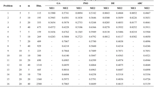
TABLE 4. The results of solving sample problems

Problem n m Dim. GA PSO DE ABC

ME1 ME2 ME1 ME2 ME1 ME2 ME1 ME2

1 5 5 115 0.1980 0.5741 0.0894 0.5182 0.0043 0.4868 0.0052 0.4867

2 5 10 195 0.3945 0.6581 0.1838 0.5646 0.0300 0.5059 0.0226 0.5031

3 5 20 355 0.3654 0.5878 0.2753 0.5248 0.0205 0.4053 0.0177 0.4041

4 5 40 675 0.4572 0.6228 0.5106 0.6366 0.0278 0.3932 0.0252 0.3911

5 7 5 159 0.3436 0.6762 0.1365 0.5949 0.0138 0.5486 0.0218 0.5504

6 7 10 269 0.4283 0.5884 0.2723 0.4792 0.0812 0.4117 0.0302 0.4050

7 7 20 489 - 0.7067 - 0.5780 - 0.4038 - 0.4096

8 7 40 929 - 0.6218 - 0.5660 - 0.4214 - 0.4246

9 10 5 225 - 0.7864 - 0.7489 - 0.7071 - 0.7051

10 10 10 380 - 0.6140 - 0.5047 - 0.4563 - 0.4521

11 10 20 690 - 0.6985 - 0.6399 - 0.4974 - 0.4944

12 10 40 1310 - 0.6859 - 0.6064 - 0.4075 - 0.4048

13 20 5 445 - 0.8016 - 0.6963 - 0.6687 - 0.6898

14 20 10 750 - 0.6684 - 0.6258 - 0.5318 - 0.5336

15 20 20 1360 - 0.5973 - 0.5791 - 0.4836 - 0.4726

16 20 40 2580 - 0.7065 - 0.6689 - 0.4615 - 0.5139

Because the model of the problem is a MILP model, the way of solving and optimizing is too time-consuming and impossible when the dimensions of the problem are too large. In order to obtain an upper bound for each generated problem, the binary and integer conditions are eliminated from the model’s variables, and accordingly an optimal solution to linear programming (LP) is obtained for each of the problems. Then, the first error index (E1), which is the ratio of the metaheuristic solution to the optimal solution, and the second error index (E2), which is the ratio of the metaheuristic solution to the calculated upper bound, are calculated according to Equations (50) and (51). In these equations, X is the result of metaheuristic solving, A is the result of solving the MILP model, and

B is the calculated upper bound.

1 A X

E A

-= (50)

2 B X

E B

-= (51)

The results of solving 160 generated problems (10 problems for each of 16 compositions) are mentioned in Table 4. The table shows the average values of error indexes (ME1, ME2), which are obtained from metaheuristic solving of 10 problems for each composition. Also, Figure 5 shows the average value of

the error indexes (TME1, TME2), resulting from metaheuristc solving of all the generated problems. As it seems in Figure 5, ABC method results in the best solution, and by taking the large dimensions of the problems into account, the average of its first error index is an acceptable value (2%). In this method, the second error index varies about 0.5 in value. However, the second index cannot be used to evaluate the efficiency of ABC method but as it remains approximately at the same value as for small problems, it is concluded that the performance of ABC method does not decline once the problem is enlarged.

Figure 5. The total average of error indexes

0.66

0.60

0.49 0.49

0.36

0.24

0.03 _0.02

0.00 0.10 0.20 0.30 0.40 0.50 0.60 0.70 0.80

GA PSO DE ABC

Algorithms

T

ot

al

M

ea

n

of

E

rr

or

I

nd

ex

es

6. CONCLUSION

In this paper, a CLSC is planned for ordering, production, and delivery operations. Considering ordering, holding and shortage costs, the times and capacities of shipment and production operations, and the capacity conditions of warehouses, this work tried to consider a more real problem. Also, the current study is done, especially for high-tech products.

Having presented the problem, this paper defines a structure for evaluating the solutions and puts forward four metaheuristic algorithms including GA, PSO, DE, and ABC with some modifications to solve the model. Comparing error values, the paper concludes that ABC algorithm has a relatively more acceptable error value; which has the minimum error value among all the other explored algorithms. The results of this study indicated an approximate solution for selecting active markets among potential markets and for determining the time and quantity of components and products to produce and ship in a CLSC in general, and for high-tech products in particular, by dividing the time horizon into many periods, which increase the accuracy of planning. Since the model is considered for single-objective optimization, the multi-objective model may be considered for further studies in this regard. The probabilistic demand pattern may also be considered in the future study.

7. REFERENCES

1 Sadegheih, A., Drake, P., Li, D. and Sribenjachot, S., "Global supply chain management under the carbon emission trading program using mixed integer programming and genetic algorithm", International Journal of Engineering,

Transactions B: Applications, Vol. 24, (2011), 37-53.

2 Sahraeian, R., Bashiri, M. and Taheri Moghadam, A., "Capacitated multimodal structure of a green supply chain network considering multiple objectives", International Journal

of Engineering, Transactions C: Aspects, Vol. 26, (2013),

963-974.

3 Wang, L. and Murata, T., "Study of optimal capacity planning for remanufacturing activities in closed-loop supply chain using system dynamics modeling", IEEE International Conference on Automation and Logistics (ICAL), Chongqing, China, (2011). 4 Mitra, S., "Inventory management in a two-echelon closed-loop

supply chain with correlated demands and returns",Computers & Industrial Engineering, Vol. 62, (2012), 870-879.

5 Zhou, G. and Min, H., "Designing a closed-loop supply chain with stochastic product returns: a Genetic Algorithm approach", InternationalJournal of Logistics Systems and Management, Vol. 9, (2011), 397-418.

6 Du, L., Wu, J. and Hu, F., "Logistics network design and optimization of closed-loop supply chain based on mixed integer nonlinear programming model", ISECS International Colloquium on Computing, Communication, Control, and Management, Sanya, China, (2009).

7 Mirzahosseinian, H., Makui, A., Teimoury, E., Ranjbar-Bourani, M. and Amoozad-Khalili, H., "Impact of transportation system on total cost in a two-echelon dual channel supply chain", International Journal of Engineering, Transactions B: Applications, Vol. 24, (2011), 27-36.

8 Mungan, D., "An optimal operational policy for an integrated production-delivery system under continuous price decrease", Master Thesis, Louisiana State University, USA, (2007). 9 Hassanzadeh Amin, S. and Zhang, G., "An integrated model for

closed-loop supply chain configuration and supplier selection: Multi-objective approach", Expert Systems with Applications, Vol. 39, (2012), 6782–6791..

10 Esteves, V.M., Sousa, J.M., Silva, C.A., Povoa, A. and Gomes, M., "SCant-design: Closed loop supply chain design using ant colony optimization", IEEE Congress on Evolutionary Computation (CEC), Brisbane, Australia, (2012).

11 Yang, P., Chung, S., Wee, H., Zahara, E. and Peng, C., "Collaboration for a closed-loop deteriorating inventory supply chain with multi-retailer and price-sensitive demand",

International Journal of Production Economics, Vol. 143,

(2013), 557-566.

12 Zeballos, L.J., Mendez, C.A., Barbosa-Povoa, A.P. and Novais, A.Q., "Multi-stage stochastic optimization of the design and planning of a Closed-Loop Supply Chain", 23rd European Symposium on Computer Aided Process Engineering, Lappeenranta, Finland, (2013).

13 Georgiadis, P. and Athanasiou, E., "Flexible long-term capacity planning in closed-loop supply chains with remanufacturing",

European Journal of Operational Research, Vol. 225, (2013),

44-58.

14 Zeballos, L.J., Mendez, C.A., Barbosa-Povoa, A.P. and Novais, A.Q., "Multi-period design and planning of closed-loop supply chains with uncertain supply and demand", Computers &

Chemical Engineering, (2014).

15 Yu, J., Sarker, B.R., Mungan, D. and Rahman, M., "A production-delivery inventory system under continuous price decrease and finite planning horizon", Industrial Engineering Research Conference, Vancouver, Canada, (2008).

16 Bing-Chang, O. and Yi-Ming, F., "JIT delivery policy for a supply chain under continuous price decrease", Eighth International Conference of Chinese Logistics and Transportation Professionals, Chengdu, China, (2008).

17 Yu, J.C., Tsai, M., Liour, Y. and Cheng, N., "An efficient supplier-buyer partnership for hi-tech industry", International Conference on New Trends in Information and Service Science, Beijing, China, (2009).

18 Yu, J., Mungan, D. and Sarker, B.R., "An integrated multi-stage supply chain inventory model under an infinite planning horizon and continuous price decrease", Computers & Industrial

Engineering, Vol. 61, (2011), 118-130.

19 Georgiadis, P., Vlachos, D. and Tagaras, G., "The impact of product lifecycle on capacity planning of closed-loop supply chains with remanufacturing", Production and Operations

Deterministic and Metaheuristic Solutions for Closed-loop Supply Chains with

Continuous Price Decrease

H.R. Kamali, A. Sadegheih, M.A. Vahdat-Zad, H. Khademi-Zare

Department of Industrial Engineering, University of Yazd, Yazd, Iran

P A P E R I N F O

Paper history:

Received 28 February 2014 Received in revised form 11 May 2014 Accepted 14 August 2014

Keywords:

Closed-loop Supply Chain Continuous Price Decrease NP-hard

Metaheuristic

هﺪﯿﮑﭼ

تﺎﻣﺪﺧﻪﺋاراﺎﯾتﻻﻮﺼﺤﻣﺪﯿﻟﻮﺗرﻮﻈﻨﻣﻪﺑارﺎﻬﻧﺎﻣزﺎﺳ،ﺖﺑﺎﻗرﯽﻠﺻاﻪﺘﺴﻫناﻮﻨﻋﻪﺑارﺎﮐﻦﯿﻣﺎﺗهﺮﯿﺠﻧزﮏﯾ،ﯽﻧﺎﻬﺟدﺎﺼﺘﻗارد ﯽﻣﺖﯾﻮﻘﺗﻢﮐﻪﻨﯾﺰﻫﺎﺑﺰﯿﻧوبﻮﻠﻄﻣﺖﯿﻔﯿﮐﺎﺑ،ﺐﺳﺎﻨﻣنﺎﻣزرد ﺪﯾﺎﻤﻧ

. ﺪﻨﭼ،ﯽﻟﻮﺼﺤﻣﮏﺗﻪﺘﺴﺑﻪﻘﻠﺣﻦﯿﻣﺎﺗهﺮﯿﺠﻧزﻪﻟﺎﻘﻣﻦﯾا

،ﯽﺤﻄﺳ و هرودﺪﻨﭼ ﺤﻣياﺮﺑاريا ﮏﯾژﻮﻟﻮﻨﮑﺗتﻻﻮﺼ

) ﺪﻧرادﯽﻟوﺰﻧﻪﺘﺳﻮﯿﭘﺖﻤﯿﻗﻪﮐ (

ﻪﻣﺎﻧﺮﺑ يﺰﯾر هدﺮﮐ ياﺮﺑﺖﯾﺎﻬﻧردو

ﻢﯿﻤﺼﺗتﺎﻌﻄﻗوتﻻﻮﺼﺤﻣماﺪﻬﻧاوﻊﯾزﻮﺗ،ﺪﯿﻟﻮﺗ،ﻦﯿﻣﺎﺗ ﯽﻣيﺮﯿﮔ

ﺪﯾﺎﻤﻧ . ﻪﻣﺎﻧﺮﺑلﺪﻣﻞﺣياﺮﺑ ﺢﯿﺤﺻدﺪﻋﻂﻠﺘﺨﻣﯽﻄﺧيﺰﯾر

ااﺮﻓشوررﺎﻬﭼﻪﻟﺎﻘﻣﻦﯾاردﯽﺳرﺮﺑدرﻮﻣﻪﺘﺴﺑﻪﻘﻠﺣﻦﯿﻣﺎﺗهﺮﯿﺠﻧزﻪﺑطﻮﺑﺮﻣ ﻪﻨﯿﻬﺑ،ﮏﯿﺘﻧژﻢﺘﯾرﻮﮕﻟايرﺎﮑﺘﺑ

،تارذهﻮﺒﻧايزﺎﺳ

ﺖﺳاهﺪﯾدﺮﮔدﺎﻬﻨﺸﺒﭘﯽﻋﻮﻨﺼﻣيﺎﻫرﻮﺒﻧزﯽﻧﻮﻟﻮﮐو،ﯽﻠﺿﺎﻔﺗﻞﻣﺎﮑﺗ .

ﻞﺻﺎﺣﺞﯾﺎﺘﻧﺎﺑشوررﺎﻬﭼﻦﯾاﯽﺗﺎﺒﺳﺎﺤﻣﺞﯾﺎﺘﻧﺖﯾﺎﻬﻧرد

ﺖﺳاهﺪﺷﻪﺴﯾﺎﻘﻣﻪﻟﺎﺴﻣلﺪﻣﻪﻨﯿﻬﺑﻞﺣزا .

ﯽﻣنﺎﺸﻧﺞﯾﺎﺘﻧ يدﺮﮑﻠﻤﻋيارادﯽﻋﻮﻨﺼﻣيﺎﻫرﻮﺒﻧزﯽﻧﻮﻟﻮﮐشورﻪﮐﺪﻫد

زابﻮﺧ

ظﺎﺤﻟ ﯽﻣباﻮﺟﺖﯿﻔﯿﮐ ﺪﺷﺎﺑ

.