Response Surface Methodology Approach to the Optimization of Cyclone Separator Geometry for Maximum Collection Efficiency

Vol.9 (2019) No. 4

ISSN: 2088-5334

Response Surface Methodology Approach to the Optimization of

Cyclone Separator Geometry for Maximum Collection Efficiency

Yunardi

, Umi Fathanah

, Edi Munawar

, Bayu Pramana Putra

, Asbar Razali

, Novi Sylvia

#

Chemical Engineering Dept., Universitas Syiah Kuala, Banda Aceh, Indonesia 23111 E-mail: * [email protected]

+

Mechanical Engineering Dept., Universitas Syiah Kuala, Banda Aceh, Indonesia 23111

$

Chemical Engineering Dept., Malikussaleh University, Lhokseumawe, Indonesia

Abstract

—

treatments were performed following Box-Behnken experimental design of seven factors and three levels (-1, 0 and +1). The response variable, the cyclone collection efficiency, was calculated in accordance with the Muschelknautz model using a spreadsheet software. The relationship between the response variable and independent variables was mathematically expressed according to a quadratic polynomial equation calculated with the aid of Design Expert software. The results of the research showed that among seven variables being investigated, there are only five cyclone geometry parameters which significantly affected the cyclone collection

efficiency, including inlet height (a/D), inlet width (b/D), vortex finder height (S/D), vortex finder diameter (De/D) and total cyclone

height (Ht/D). The optimization was then conducted to include these five variables that significantly affected the collection efficiency

and neglected the remaining other two variables. The optimization computation was run in the Design Expert statistical software by setting a maximum possible value for the collection efficiency. The maximum collection efficiency of 91.244% was obtained when the independent variables of inlet height a/D=0.8, inlet width b/D=0.38, vortex finder height S/D=0.69, vortex finder diameter

De/D=0.575 and total cyclone height Ht/D=3.12. Validation of this statistical finding was tested again and compared with the result of

Muschelknautz model calculation to give a significantly small error of 0.82%.

Keywords— box-behnken; design experiment; particle; muschelknautz model; RSM; factor; calculation.

I. INTRODUCTION

Cyclone separator is one of the most frequently used equipment to control gas dust emissions in process industries. Cyclones when it compared to other air pollution control equipment, are more preferred due to their simplicity in design, low manufacturing and maintenance costs and reliable at elevated temperature and pressure ranges. Even though cyclones are more widely used as a final collector to remove large particles, they are also frequently employed as an initial particle separator to further streamline other particle-collecting devices such as electrostatic precipitators, scrubbers or fabric filters [1].

The main performance of a cyclone is determined by its particle collection efficiency and pressure drop. Consequently, the higher the efficiency of dust particle collection and the lower the pressure drop, the better the cyclone performance, and vice versa. The evaluation of a

models is still considered useful in the design or evaluation the performance of a cyclone.

Various models of theoretical and semi-empirical models have been developed to assess the performance of cyclones [3]–[5]. The accuracy of the mathematical equations of these models greatly depends on how well the assumptions used in describing events occurring within the cyclone. It is therefore not surprising if there are semi-empirical models, which give predictive results that is much distorted from the experimental measurements [6]. Among the current available mathematical models for the design of cyclone, the Muschelknautz Model is the most practical and reliable model for predicting and assessing the cyclone performance [7], [8]. The model has been developed for over the past 30 years and it is an expansion of the Barth model [4]. Compared to other models, this model provides advantages in terms of its ability to incorporate the effects of cyclone wall roughness, dust mass load, and particle size distribution changes into its mathematical models. Deng and Zhang [9] employed the model to design the geometry of a cyclone for separation of polycarbonate. They calculated the split particle size and total pressure drop with the use of this model, while the flow field inside the cyclone was simulated with CFD commercial code. Results obtained by Muschelknautz Model agree to those obtained by numerical simulation, leading to a conclusion that the Muschelknautz Model is feasible for the prediction of cyclone properties. However, it should be noted that their study was more concentrated on the prediction of pressure drop in the cyclone, instead of predicting the particle collection efficiency.

Elsayed and Lacor [10] and Brar [11] have also investigated cyclone optimization studies employing Muschelknautz Model. Response Surface Methodology approach coupled with Muschelknautz Model was used to optimize the cyclone geometry and performance in both studies. The response variable is expressed as a function of independent variables, cyclone geometric ratio. Again, similar to the study of Deng and Zhang [9], both latter studies of Elsayed and Lacor [10] and Brar [11] also aimed at optimizing the cyclone geometry to give the response variable, minimum pressure drop. Even though the parameter of particle collection efficiency in a cyclone is as important as the pressure drop, there has been very few studies reported on the optimization of cyclone geometry for maximum collection efficiency. The purpose of the present study is therefore to optimize the cyclone geometry aiming at obtaining maximum collection efficiency using the Muschelknautz cyclone model approach in combination with response surface methodology.

In the last recent years, an approach called response surface methodology (RSM) has been increasingly used as a technique to optimize a process when independent variables interact with response variables [12]. The RSM is a collection of statistical and mathematical techniques that have been successfully employed for optimization studies, including in biomass densification process [13], cyclone performance [11] and cyclone performance with particular attention to minimum pressure drop [10]. The present study reported results obtained from an optimization of cyclone

geometry employing Muschelknautz Model coupled with RSM to obtain a maximum cyclone collection efficiency.

II. MATERIAL AND METHOD

A. Model Muschelknautz

There almost no single mathematical model, which is capable of describing the physical phenomena inside a cyclone precisely, due to the complexity of the turbulent flow, involved in it. However, compared to the other mathematical models currently available for designing a cyclone, the improved Muschelknautz model has the ability to provide significantly better predictive results [9, 14]. Muschelknautz's model itself has been continuously developed so that it has a number of variants, but in this study, a model described in detailed by Hoffmann and Stein [7] has been utilized for the purpose of the design of the cyclone gas-particle separator.

According to Muschelknautz's model [7], the overall cyclone collection efficiency can be obtained by calculating the efficiency of each size fraction and multiplying it by the mass fraction of each size fraction. In the mathematical form, Equation 1 expresses the overall collection efficiency.

(

)

1

N

i i

i

MF

η η

=

=



with η is the overall efficiency, ηi efficiency of capture for

the average particle size in each fraction and ΔMFi the ith

mass fraction. Among various proposed equations to calculate the fractional efficiency, Equation 2 is one of the simplest and more practical form.

50

1

1

i m

i

x x η =

 

+ 

 

(2)

where x50 is the cut point diameter or cut size (μm), m a

constant and xi particle diameter (µm). The value of m in

Equation 2 can be obtained graphically by making a correlation between ηi and xi. However, the value of x50 has

to be calculated directly using a variation of the Barth model as shown in Equation 3.

(

)

(

)

(

)

50

18 0.9

2 fact

p t

Q

x x

v H S

CS

θ

µ

π ρ ρ

=

− − (3)

where Ht is cyclone height (m), S height of vortex finder

(m), Q inlet gas flow rate (m3/s), vθCS inner vortex tangential

velocity (m/s), ρp particle density (g/cm3), ρ air density (g/

cm3) and μ air viscosity (Pa. s). Interested readers may consult Hoffmann and Stein [7] for a more complete description of the model.

B. Procedures and Design of Experiment

The independent variables under investigation in this study cover some parameters. The parameters are related to the cyclone geometry, including inlet height, X1 = a/D, inlet

width, X2 = b/D, vortex finder length, X3 = S/D, vortex

finder diameter, X4 = De/D, cylinder height, X5 = h/D, total

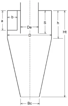
cyclone height, X6 = Ht/D and cone tip diameter, X7 = Bc/D.

symbols that state the physical characteristics of a cyclone. For a diameter (D) = 0.2 m, the cyclone wall roughness used in this simulation experiment was 0.046 mm. The response variable observed under the present study was the cyclone collection efficiency only. Calculation of collection efficiency was based on Equation 1 of the Muschelknautz model as described above and was carried out using spread sheet software by adjusting the gas flow entering the cyclone at a constant rate for each experiment, keeping a dust loading of less than 10%. The level and code of the independent variables examined in this study are shown in Table 1, while data for gas and particle characteristics entering the cyclone are presented in Table 2.

Fig. 1. A schematic diagram of cyclone geometry

Design Expert statistical software (Version 8.07, State-Ease Inc., Minneapolis, USA) was used to generate a table of experimental runs containing values of independent variables of different combination following the range pre-defined in Table 1. Sixty-two experiments run randomly to screen the independent variables that influence the response variable, cyclone collection efficiency. The analysis of variance test results show that out of the seven independent variables in Table 1 being tested, only five independent variables that have a significant effect on the response variable. Later, the run was carried out again by considering the independent variables having a significant effect and ignoring the variables that have no effect on the response variable. Forty-six run were then re-tested for five variables to optimize the independent variables. Calculated data on collection efficiency were obtained through spreadsheet software applying related formula for computing the efficiency, according to Muschelknautz Model. Results were analyzed based on response surface methodology with the help of Design Expert statistical software (Version 8.07, State-Ease Inc., Minneapolis, USA), fitting to a second order polynomial equation as shown in Equation 4.

2 0

1 1

k k

k i i ii i ij i j

n n i j

Y β βX β X β X X ε

= = <

= +







where Yk is the predicted response variable and Xi (X1, X2, X3, X4, and X5 are independent variables that influence the

response variable. The βo, βi, and βij are coefficients for

linear, quadratic and inter-variable interaction, whose values can be estimated using the least squares method and have been described in many statistical literatures [15]. The last term ɛ represents error. The RSM attempts to fit the data to a second order polynomial as Equation 4. The response could be presented in the form of three-dimensional space or contour plots. Elsayed and Lacor [10] and Brar [11] have successfully applied the second order polynomial equation in relation to the study of cyclone optimization.

TABLEI

VALUES OF INDEPENDENT VARIABLES

TABLEII

CHARACTERISTICS OF GAS AND PARTICLES

Gas Data Symbol Unit Values

Flow rate Q m3/s 0.05

Density ρ Kg/m3 1.2

Viscosity μ Pa. s 0.000018

Particle Data

Density ρp Kg/m3 2730

Bulk density ρb kg/m3 1365

Mass fraction Co Kg/Kg 0.00375

Solid loading C g/m3 4.5

For the optimization purpose, it is required to develop the optimum criteria in relation to the desirability function (DF) approach [16]. A number of aspects, including technical and economic considerations, control the maximum or minimum value of the response variable being investigated. The approach of Desirability Function, DF in optimizing the Equation 2 is to convert each response Yk into an individual

desirability function d_k =h Y

( )

value, then dk will be equal to 1 and in the case the response

falls beyond acceptable limit, dk will be equal to 0. At the

next stage, the individual desirability functions are then coupled into a single combined response, commonly called as Desirability Function (DF), expressed as Equation 5 consisting of geometric means of different dk values.

1/3 3

1

k

DF = d 



∏

Equation 5 implied that DF would be close to 1.0 in case all individual desirability functions are also close to unity. Consequently, optimum condition or target value is obtained when DF is equal or close to unity. Although in general, the desirability function approach is used to optimize

multi-Independent variables Code and value

-1 0 +1

variable response, in practical the statistical software provides a feature for single response variable. Such methodology has been successfully implemented in optimizing various processes, including mucilage extraction [17], solar air heating [18], inhibition sintering [19], densification process [13], as well as cyclone design and performance [10, 11].

III.RESULTS AND DISCUSSION

A. Analysis of variance (ANOVA)

Analysis of variance on the results of runs based on seven independent variables is presented in Table 3. The level of effect from each independent variable is strongly influenced by F values and P (probability). The greater the value of F and the smaller the value of P, the more influential of the independent variables on the response variable will be. From the ANOVA analysis in Table 3, it can be seen that the quadratic polynomial model has a significant effect, which is indicated by a relatively large F value of 87.83. The value of Prob>F for the model is smaller than 0.0001 indicating that the model is highly significant. A larger P value indicates that the factors being investigated do not have a significant effect. Now it is clear that out of seven independent variables under investigation, only five independent variables have a significant effect on cyclone collection efficiency. Those five independent variables consist of inlet height (a/D), inlet width (b/D), vortex finder length (S/D), vortex finder diameter (De /D), and total cyclone height (Ht/D). On the other hand, it can be noted that the cylinder

height (h/D) and cone tip diameter (Bc/D) do not have a

significant effect on cyclone collection efficiency. Therefore, these two parameters are ignored in the optimization of cyclone geometry parameters.

Subsequent runs were carried out by considering five influential factors and samples of calculation on the collection efficiency using the Muschelknautz model are shown in Table 4. In this table, the symbol Y1 represents the

response variable (collection efficiency) calculated using the Muschelknautz model, expressed as Equation 1. Table 5 presented analysis of variance to test the soundness of the model. Here it can be seen that the model and all major factors still have a highly significant effect on the collection efficiency. However, not all-linear interaction has significant influence on the response variables. Only the interaction of X2X4 and X3X6 that have a significant influence on the

cyclone collection efficiency.

TABLEIII

ANALYSIS OF VARIANCE FOR QUADRATIC MODEL FOR SEVEN MAIN FACTORS

Source Sum square

Df Mean square Value (F) P Value Prob(p)> F Remark

Model 6763.61 7 966.23 87.83 < 0.0001 Significant X1 1262.63 1 1262.63 114.78 < 0.0001 Significant X2 2454.25 1 2454.25 223.10 < 0.0001 Significant X3 116.71 1 116.71 10.61 0.0019 Significant X4 1768.82 1 1768.82 160.79 < 0.0001 Significant

X5 0.82 1 0.82 0.075 0.7855 Not

Significant X6 1159.83 1 1159.83 105.43 < 0.0001 Significant

X7 0.54 1 0.54 0.049 0.8262 Not

Significant

TABLEIV

SAMPLES OF CYCLONE PREDICTED EFFICIENCY USING MUSCHELKNAUTZ MODEL

Run X1 a/D X2 b/D X3 S/D X4 De/D X6 Ht/D Output data Y1 Y2 1 0.62 0.38 0.69 0.40 3.12 78.03 77.12 2 0.62 0.29 0.5 0.40 3.12 62.00 63.03

- … … … …

45 0.62 0.29 0.5 0.575 4.24 69.10 69.22 46 0.44 0.29 0.69 0.4 3.12 54.34 54.79

On the basis of the results of analisys of variance presented in Table 5, a quadratic polinomial correlation can be generated considering independent variables which significantly affect the rensponse variable, cyclone collection efficiency. Such correlation is shown as Equation 6.

[ ]

[ ]

[ ]

[ ]

[ ]

[ ][ ]

[ ][ ]

[ ][ ]

[ ][ ]

[ ][ ]

[ ]

[ ]

[ ]

1 2 3

4 6 1 2

1 4 2 4 2 6

2 2 2

4 6 1 4 6

45.26 131.58 187.22 7.78

147.32 20.13 63.67

33.20 105.61 11.06

12.89 43.22 75.70 0.71

Y X X X

X X X X

X X X X X X

X X X X X

= − + + +

+ − −

− − +

+ − − +

(6)

The model describing the relationship between the cyclone collection efficiency and the cyclone geometry parameters presented in Equation 6 is very satisfying. This is indicated by a fairly high coefficient of determination, namely R2 = 0.9951 as shown in Table 5.

TABLEV

ANALYSIS OF VARIANCE ON FIVE FACTORS AND THEIR INTERACTIONS Source Sum of

square

Df Mean square Value (F) P Value Prob(p)> F Remarks

Model 4641,51 20 232,08 256,34 < 0.0001 Significant X1 847,78 1 847,78 936,40 < 0.0001 Significant X2 1914,57 1 1914,57 2114,71 < 0.0001 Significant X3 35,02 1 35,02 38,68 < 0.0001 Significant X4 1190,41 1 1190,41 1314,84 < 0.0001 Significant X6 512,11 1 512,11 565,65 < 0.0001 Significant X1 X2 4.26 1 4.26 4.70 0.0399 Significant X1 X3 0.41 1 0.41 0.45 0.5079 Not

significant X1 X4 4.37 1 4.37 4.83 0.0375 Significant X1 X6 2.60 1 2.60 2.88 0.1024 Not

significant X2 X3 0.89 1 0.89 0.98 0.3313 Not

significant X2 X4 11.07 1 11.07 12.22 0.0018 Significant X2 X6 4.98 1 4.98 5.50 0.0273 Significant X3 X4 0.28 1 0.28 0.31 0.5843 Not

significant X3 X6 0.55 1 0.55 0.61 0.4427 Not

significant X4 X6 25.55 1 25.55 28.22 < 0.0001 Significant X12 _{15.29 1 15.29 16.89 0.0004 Significant}

X22 _{1.33 1 1.33 1.47 0.2360 Not}

significant X32 _{0.010 1 0.010 0.011 0.9167 Not}

significant X42 _{43.86 1 43.86 48.44 < 0.0001 Significant} X62 _{8.24 1 8.24 9.10 0.0058 Significant}

calculated data and the prediction by the model is in closer agreement. Since the value of R2 from this study is 0.9951, which is very close to unity, meaning that the prediction of cyclone efficiency by Equation 6 will be very close to the calculated cyclone efficiency using Muschelknautz model. However, it should be noted that a large R2 value does not always reflect the perfection of the regression model. Adding another variable to the model will always increase the value of R2, regardless of whether the independent variable has an effect on the response variable. Therefore, the value of adjusted (adj.) R2 is more likely to be used to evaluate the fittingness of the model. Koocheki et al. [17] suggest that this value must be greater than 0.9. As can be seen in Table 5, the value of adj. R2 is significantly much greater than 0.9. In addition to the adj. R2, a predicted (pred) R2 value to measure how well a model predicts responses for new observations and it is expected that the value be close to unity.

T

If adequate (adeq) precision is put into consideration in analysing the soundness of the model, then a value of greater than 4.0 is needed to describe the fitness of the model. The adequate precision test is a measure of signal to noise ratio. It compares the number of the predicted values at the design points to the average prediction error. A ratio of greater than 4 indicates adequate model discrimination [17]. In this case, the value of adequate precision is significantly convincing which is equal to 62,097, 20 times greater than the minimum expected value of 4.

The coefficient of variation (CV) provides an overview of the precision of the data points on a series of data around the mean value. In general, the greater the value of CV means that there is a high variation of data around the average value so that the reliability of the experiment is low. Therefore, a low CV value is something that is expected to ensure the ability of the model to produce conformity of predictive results with calculated data. Here the CV value is quite low at 1.28%, meaning data distribution is to have very low variance. Therefore, statistical explanations indicate that the model shown in Equation 6 is very reliable. However, a proof is required to make sure that the predicted values using Equation 6 are in agreement with the calculations using Muschelknautz model, by making a comparison. A few data for comparison are presented in Table 4, of which Y1 and Y2

are values of variable response calculated using Muschelknautz model and predicted using Equation 6. It is observed that the error for each comparison on average is less than 1%. This proves that predictions are significantly in agreement with Muschelknautz model calculation data.

B. Interaction Between Cyclone Geometry Variables

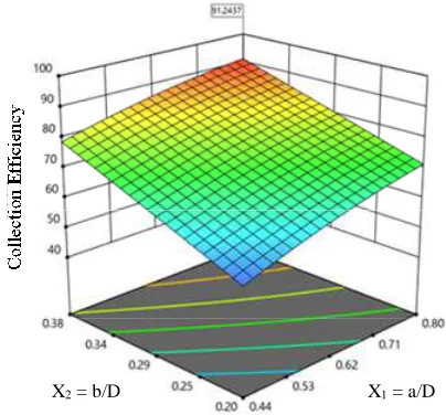
Three dimensional response surfaces demonstrated interaction between cyclone geometry variables are presented in Fig. 2 and 3. Fig. 2 illustrates the interaction between height (X1) and inlet width (X2) on the cyclone

collection efficiency, when vortex finder height, X3 =0.69,

vortex finder diameter X4=0.575 and total cyclone height

X6=3.12. Fig. 2 indicates that the interaction between X1 and

X2 on the collection efficiency was analysed when all other

influential parameters of X3, X4 and X6 are at optimum

condition. In accordance to Fig. 2, the higher particle

collection efficiency in the cyclone was achieved with the increase of inlet height and inlet width. At the inlet height parameter, X1=0.80 and X2=0.38, an optimum particle

collection efficiency of 91.24% was obtained which satisfies the desirability function DF of 0.995, very close to unity. In this study, the gas flow rate entering the cyclone was kept constant at 0.05 m3/s. With the increase values of X1 and X2,

consequently the inlet velocity become reduced allowing particles to have longer residence time in the cyclone, to have more chance to settle down and to have less chance of entrainment. As a result, the particle collection efficiency becomes higher. Such result was also confirmed by experimental works of Fualkner and Shaw [20] who suggested that cyclone employed in agricultural industries could be operated at lower inlet velocities in order to obtain the collection efficiency equal to those predicted by Texas A & M Cyclone Design (TCD) method. In addition to increasing efficiency, lowering the velocity was also reducing the pressure drop [20], leading to a saving in the operational cost of the cyclone.

Fig 2 Response surface plot showing the effect of inlet height (X1) and inlet width (X2) on the cyclone collection efficiency

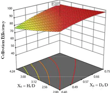
Fig 3 presents the relationship between the change in the parameters of the vortex finder diameter (X4) and total

height of a cyclone (X5) on the particle collection efficiency,

when other influential cyclonic parameters such as inlet height, X1, inlet width, X2 and vortex finder height, X3 are at

their optimum condition of 0.80, 0.38, and 0.69, respectively. From Fig. 3, it can be seen that when the total cyclone height (X6) is decreased until 2.00 and the diameter of vortex finder

(X4) is increased up to 0.75, the collection efficiency of the

cyclone increases reaching the maximum at 97.75 %. However, for the purpose of optimization, the maximum or optimum collection efficiency has to satisfy as such that DF is equal or close to unity. Even though, the value of the collection efficiency is high enough, it does not meet the DF requirement when it is crosschecked from Fig. 4. Fig 4 illustrates the response surface of Desirability Function, DF with respect to the change of cyclone geometric parameters of vortex finder diameter (X4) and total cyclone height (X6).

Comparing Fig 3 and Fig 4, the maximum efficiency from Fig 3 is achieved when values of X6 = 2.0 and X4 = 0.75.

Unfortunately, inspecting Fig 4, at these values (X6 = 2.0

and X4 = 0.75), it is clearly seen that the value of DF is 0.42,

far from unity. As a consequent, this cannot be accepted as the optimum particle collection efficiency of the cyclone. Still from Fig. 4, the highest value of DF = 0.995 was achieved when X4 = 0.575 and X6 =3.12.

X6 = Ht/D X4 = De/D

Fig 3. Response surface plot showing the effect of vortex finder diameter and total cyclone height on the cyclone collection efficiency

X6 = Ht/D

2.00 2.56 3.12 3.68 4.24

0.40 0.49 0.57 0.66 0.75 0.000

0.200 0.400 0.600 0.800 1.000

D: De/D 0.995 0.995

X4 = De/D

Fig 4. Response surface plot illustrating the effect of vortex finder diameter and total cyclone height on the Desirability, DF.

Turning back to Fig 3, at the geometry parameters of total cyclone height equals to 3.12 and vortex finder diameter equals to 0.575, the particle collection efficiency of 91.244% was obtained. Since this condition is, in accordance to the condition, that DF is equal or close to unity, consequently this particle collection efficiency could be determined as the optimum collection efficiency of the cyclone.

C. Optimization of Geometry Parameters

The main objective of this study was to optimize the cyclone geometry to give the maximum response value, cyclone collection efficiency. Out of the 15 solutions offered by Design Expert software, the first three alternatives were included in Table 6. Those alternatives are having similar desirability function value close to unity. Desirability function is one of the best ways to optimize the independent variables in an attempt to gain the desired response value. The desirability function (DF) has a value of between 0 and 1, If DF value is equal to 0, the response desire is not

achieved at all and on the contrary if the DF value is equal to or close to 1.0, the response desire is reached. From Table 6, it can be observed that all alternatives provide a value of DF close to one, but with different collection efficiency. Alternative 1 provides the highest and the closest DF values to unity, 0.955 and similar performance in terms of collection efficiency of around 91%. Therefore, it is judicious to take this alternative as an optimum condition with a collection efficiency of 91.244% on condition of independent variables a/D = 0.8; b/D = 0.38; S/D = 0.69; De/D = 0.575 and Ht/D = 3.12

TABLEVI

OPTIMUMALTERNATIVESANDDESIRABILTYFUNCTION ACCORDINGTORSM

No a/D b/D S/D De/D Ht/D η DF

1 0.8 0.38 0.69 0.575 3.12 91.244 0.995 2 0.798 0.380 0.69 0.575 3.12 91.281 0.994 3 0.80 0.378 0.69 0.575 3.12 91.306 0.994

IV. CONCLUSIONS

Response surface methodology (RSM) in combination with statistical analysis has demonstrated to be a valuable tool for optimizing the geometry parameters of a cyclone. The present most sophisticated semi-empirical Muschelknautz Model coupled with RSM can be easily implemented to design a cyclone of having high collection efficiency using simple spreadsheet software and Design Expert statistical commercial code. The optimization results show that the maximum collection efficiency of 91.244% can be obtained if the geometry parameters of a cyclone, such as inlet height of a/D = 0.80, inlet width b/D = 0.38, vortex finder height S/D = 0.69, vortex finder diameter De/D

= 0.575, and total cyclone height Ht/D=3.12. Re-examination

of the result of optimization using Equation 5 was compared to the calculation of the Muschelknautz Model under similar independent variables and found that comparison produced a significantly small error of 0.82% on average. Further experimental laboratory research is required to validate this result with real experimental data.

ACKNOWLEDGEMENTS

The authors express their gratitude to the Ministry of Research Technology and Higher Education of the Republic of Indonesia and Syiah Kuala University for their financial support through Prioritized Basic Research for Higher Education Institution Scheme, under Contract No: 49/UN11.2/PP/SP3/2018. Comments and suggestions on the draft of this paper from Prof. Marwan of the Department of Mathematics, Syiah Kuala University are very much appreciated.

REFERENCES

[1] Swamee P.K, Aggarwal N, Bhobhiya K. “Optimum Design of Cyclone Separator”, AIChE., vol. 55, pp.2279–2283, 2009. [2] Altmeyer, S., Mathieu, V. Jullemier, S. Contal, P. Midoux, N., S.

Rode, S., Leclerc J.-P., “Comparison of different models of cyclone prediction performance for various operating conditions using a general software”, Chem. Eng. Process, vol. 43, pp. 511–522, 2004. [3] Shepherd C. B, Lapple C.E., “Flow Pattern and Pressure Drop in

[4] Barth W., “Design and Layout of the Cyclone Separator on the Basis of New Investigations”. Brenn. Warme Kraft, vol. 8, pp. 1-9, 1956. [5] Stairmand C. J. “The Design and Performance of Cyclone

Separators”. Trans. Inst. Chem. Eng., vol. 29, pp. 357-383, 1951. [6] Mohamed-Swaray, S.G, Hamdullapur, F., “A new semi-empirical

model for predicting particulate collection efficiency in low-to-high temperature gas cyclone separators” Advanced Powder Technol., vol.15 (2), pp. 137– 164, 2004,

[7] Hoffmann A.C, Stein L.E., Gas Cyclones and Swirl Tubes Principle, Design and Operation. New York: Springer-Verlag Berlin Heidelberg. pp 111-137, 2008.

[8] Muschelknautz, E and Krambrock, W., “Design of cyclone separators in the engineering practice”, Staub-Reinhalt. Luft, vol. 30, pp. 1-12, 1970.

[9] Deng. Q.-F. Zhang, -L., “Application of Muschelknautz models in design of cyclone”, Journal of Central South University (Science and Technology), vol. 42(4), pp. 977-983, 2011.

[10] Elsayed K, Lacor C., “Optimization of the Cyclone Separator Geometry for Minimum Pressure Drop Using Mathematical Models and CFD Simulations”. Chem. Eng. Sci. vol. 65 (22), pp. 6048-6058, 2010.

[11] Brar, L. S., “Application of response surface methodology to optimize the performance of cyclone separator using mathematical models and CFD simulations” Materials Today: Proceedings, vol. 5, pp. 20426–20436, 2018.

[12] Tang D.S, Tian Y.J, He Y.Z, Li L, Hu S.Q, Li B., “Optimisation of Ultrasonic-assisted Protein Extraction from Brewer’s Spent Grain”. Czech J. Food Sci., vol. 28, pp. 9-17, 2010.

[13] Yunardi, Zulkifli, Masrianto. “Response Surface Methodology Approach to Optimizing Process Variables for The Densification of

Rice Straw as a Rural Alternative Solid Fuel”, J. Appl Sci, vol. 11, pp. 1192-1198, 2011.

[14] Rong-shan, B., Zhen-xing, W., Yu-gang, L., Xin-shun, T., Shi-qing, Z., Zhen-dong, L, Wen-wu, C., “Study on a New type of Gas-Liquid Cyclone used in COIL”, Proceedings of the 11th International Symposium on Process Systems Engineering, 15-19 July 2012, Singapore, pp. 565-569, 2012.

[15] Lazic, Z.R., Design of Experiment in Chemical Engineering: A Practical Guide. New York: Wiley-VCH, 2004.

[16] Derirnger, G and Suich, R., “Simultaneous optimization of several response variables, J. Qual. Technol., vol. 12, pp. 214-219, 1980. [17] Koocheki A, Mortazavi S.A, Shahidi F, Razavi S.M.A, Kadkhodaee

R, Milani J.M., “Optimization of Mucilage Extraction from Qodume Shirazi Seed (Alyssum Homolocarpum) Using Response Surface Methodology”. J. Food Proc. Eng., vol. 33, pp. 861-882, 2010. [18] Bootan, S., Qader, E.E, Supeni, M.K., Ariffin A.R., Abu Talib,

“RSM approach for modeling and optimization of designing parameters for inclined fins of solar air heater”, Renewable Energy vol. 136, pp. 48-68, 2019.

[19] Baligidad, S.M., Chandrasekar, U., Elangovan, K, Snahkar, S. “RSM Optimization of Parameters influencing Mechanical properties in Selective Inhibition Sintering” Materials Today, vol. 5 (2), 4903– 4910, 2018.

[20] Faulkner, B., Shaw, B.W., “Efficiency and Pressure Drop of Cyclones across a Range of Inlet Velocities”, Applied Engineering in Agriculture, vol. 22(1), pp. 155-161, 2006.