The Thirty-Third AAAI Conference on Artificial Intelligence (AAAI-19)
DDFlow: Learning Optical Flow with Unlabeled Data Distillation
Pengpeng Liu,
†∗Irwin King,
†Michael R. Lyu,
†Jia Xu
§†The Chinese University of Hong Kong, Shatin, N.T., Hong Kong
§Tencent AI Lab, Shenzhen, China
{ppliu, king, lyu}@cse.cuhk.edu.hk, [email protected]
Abstract
We present DDFlow, a data distillation approach to learning optical flow estimation from unlabeled data. The approach distills reliable predictions from a teacher network, and uses these predictions as annotations to guide a student network to learn optical flow. Unlike existing work relying on hand-crafted energy terms to handle occlusion, our approach is data-driven, and learns optical flow for occluded pixels. This enables us to train our model with a much simpler loss func-tion, and achieve a much higher accuracy. We conduct a rig-orous evaluation on the challenging Flying Chairs, MPI Sin-tel, KITTI 2012 and 2015 benchmarks, and show that our approach significantly outperforms all existing unsupervised learning methods, while running at real time.
Introduction
Optical flow estimation is a core computer vision build-ing block, with a wide range of applications, includbuild-ing au-tonomous driving (Menze and Geiger 2015), object tracking (Chauhan and Krishan 2013), action recognition (Simonyan and Zisserman 2014) and video processing (Bonneel et al. 2015). Traditional approaches (Horn and Schunck 1981; Brox et al. 2004; Brox and Malik 2011) formulate opti-cal flow estimation as an energy minimization problem, but they are often computationally expensive (Xu, Ranftl, and Koltun 2017). Recent learning-based methods (Doso-vitskiy et al. 2015; Ranjan and Black 2017; Ilg et al. 2017; Hui, Tang, and Loy 2018; Sun et al. 2018) overcome this issue by directly estimating optical flow from raw images using convolutional neural networks (CNNs). However, in order to train such CNNs with high performance, it requires a large collection of densely labeled data, which is extremely difficult to obtain for real-world sequences.
One alternative is to use synthetic datasets. Unfortu-nately, there usually exists a large domain gap between the distribution of synthetic images and natural scenes (Liu et al. 2008). Previous networks (Dosovitskiy et al. 2015; Ranjan and Black 2017) trained only on synthetic data turn to overfit, and often perform poorly when they are directly evaluated on real sequences. Another promising direction is to learn from unlabeled videos, which are readily available
∗
Work mainly done during an internship at Tencent AI Lab. Copyright c2019, Association for the Advancement of Artificial Intelligence (www.aaai.org). All rights reserved.
𝐼1
(𝑥1, 𝑦1)
𝐼2 (𝑥
2, 𝑦2)
𝐼 2
𝐼 1 (𝑥1, 𝑦1)
Teacher Model
Student Model
Flow
Flow Guide
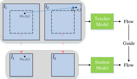
Figure 1: Data distillation illustration. We use the optical flow predictions from our teacher model to guide the learn-ing of our student model.
at much larger scale. (Jason, Harley, and Derpanis 2016; Ren et al. 2017) employ the classical warping idea, and train CNNs with a photometric loss defined on the difference be-tween reference and warped target images. Recent methods propose additional loss terms to cope with occluded pixels (Meister, Hur, and Roth 2018; Wang et al. 2018), or utilize multi-frames to reason occlusion (Janai et al. 2018). How-ever, all these methods rely on hand-crafted energy terms to regularize optical flow estimation, lacking key capability to learn optical flow of occluded pixels. As a result, there is still a large performance gap comparing these methods with state-of-the-art fully supervised methods.
Is it possible to learn optical flow in a data-driven way, while not using any ground truth at all? In this paper, we ad-dress this issue by a data distilling approach. Our algorithm optimizes two models, a teacher model and a student model (as shown in Figure 1). We train the teacher model to es-timate optical flow for non-occluded pixels (e.g., (x1, y1)
in I1). Then, we hallucinate flow occlusion by cropping
patches from original images (pixel (x1, y1)now becomes
occluded inIe1). Predictions from our teacher model are used
Forward Flow w𝑓 Backward Flow w𝑏 Backward Occlusion
𝑂 𝑏
Forward Occlusion
𝑂 𝑓 Teacher Model Teacher Model Student Model Student Model Forward-backward consistency check Forward-backward consistency check 𝐼1 & 𝐼2 𝐼2 & 𝐼1
𝐼 2 & 𝐼 1 𝐼 1 & 𝐼 2
𝐼2 𝐼1 𝐼2 𝐼1 Cropped Occlusion
𝑂𝑏𝑝
Cropped Occlusion 𝑂𝑓 𝑝 Valid Mask 𝑀𝑓 Valid Mask 𝑀𝑏 Warped Image
𝐼1𝑤
Warped Image
𝐼2𝑤
Warped Image
𝐼 1𝑤
Warped Image
𝐼 2𝑤 Image Warp Image Warp Photometric Loss Photometric Loss Loss for Occluded Pixels Forward Flow w𝑓 Backward Flow w𝑏 Backward Occlusion 𝑂𝑏 Forward Occlusion 𝑂𝑓
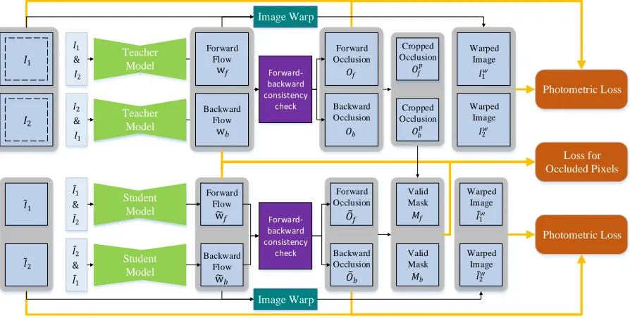
Figure 2: Framework overview of DDFlow. Our teacher model and student model have identical network structures. We train the teacher model with a photometric lossLpfor non-occluded pixels. The student model is trained with bothLp andLo, a loss for occluded pixels.Loonly functions on pixels that are non-occluded in original images but occluded in cropped patches
(guided byValid MaskMf,Mb). During testing, only the student model is used.
The resulted self-training approach yields the highest ac-curacy among all unsupervised learning methods. At the time of writing, our method outperforms all published un-supervised flow methods on the Flying Chairs, MPI Sin-tel, KITTI 2012 and 2015 benchmarks. More notably, our method achieves a Fl-noc error of 4.57% on KITTI 2012, a Fl-all error of 14.29% on KITTI 2015, even outper-forming several recent fully supervised methods which are fine-tuned for each dataset (Dosovitskiy et al. 2015; Ran-jan and Black 2017; Bailer, Varanasi, and Stricker 2017; Zweig and Wolf 2017; Xu, Ranftl, and Koltun 2017).
Related Work
Optical flow estimation has been a long-standing challenge in computer vision. Early variational approaches (Horn and Schunck 1981; Sun, Roth, and Black 2010) formulate it as an energy minimization problem based on brightness con-stancy and spatial smoothness. Such methods are effective for small motion, but tend to fail when displacements are large.
Later, (Brox and Malik 2011; Weinzaepfel et al. 2013) in-tegrate feature matching to tackle this issue. Specially, they find sparse feature correspondences to initialize flow estima-tion and further refine it in a pyramidal coarse-to-fine man-ner. The seminal work EpicFlow (Revaud et al. 2015) in-terpolates dense flow from sparse matches and has become a widely used post-processing pipeline. Recently, (Bailer, Varanasi, and Stricker 2017; Xu, Ranftl, and Koltun 2017) use convolutional neural networks to learn a feature em-bedding for better matching and have demonstrated superior
performance. However, all of these classical methods are of-ten time-consuming, and their modules usually involve spe-cial tuning for different datasets.
The success of deep neural networks has motivated the development of optical flow learning methods. The pioneer work is FlowNet (Dosovitskiy et al. 2015), which takes two consecutive images as input and outputs a dense opti-cal flow map. The following FlowNet 2.0 (Ilg et al. 2017) significantly improves accuracy by stacking several basic FlowNet modules together, and iteratively refining them. SpyNet (Ranjan and Black 2017) proposes to warp images at multiple scales to handle large displacements, and intro-duces a compact spatial pyramid network to predict optical flow. Very recently, PWC-Net (Sun et al. 2018) and Lite-FlowNet (Hui, Tang, and Loy 2018) propose to warp fea-tures extracted from CNNs rather than warp images over different scales. They achieve state-of-the-art results while keeping a much smaller model size. Though promising per-formance has been achieved, these methods require a large amount of labeled training data, which is particularly diffi-cult to obtain for optical flow.
(a)I1 (b) wf (c) wb (d)Of (e)Ob (f)Mf
(g)Ie1 (h)wef (i)web (j)Oef (k)Oeb (l)Mb
Figure 3: Example intermediate results from DDFlow on KITTI. (a) is the first input image; (b,c) are forward and backward flow; (d,e) are forward and backward occlusion maps. (g) is the cropped patch of (a); (h,i,j,k) are the corresponding forward flow, backward flow, forward occlusion map and backward occlusion map respectively. (f,l) are forward and backward valid mask, where 1 means the pixel is occluded in (g) but non-occluded in (a), 0 otherwise.
One promising direction is to develop unsupervised learn-ing approaches. (Jason, Harley, and Derpanis 2016; Ren et al. 2017) construct loss functions based on brightness con-stancy and spatial smoothness. Specifically, the target image is warped according to the predicted flow, and then the dif-ference between the redif-ference image and the warped image is optimized using a photometric loss. Unfortunately, this loss would provide misleading information when the pixels are occluded.
Very recently, (Meister, Hur, and Roth 2018; Wang et al. 2018) propose to first reason occlusion map and then ex-clude those ocex-cluded pixels when computing the photomet-ric difference. Most recently, (Janai et al. 2018) introduce an unsupervised framework to estimate optical flow using a multi-frame formulation with temporal consistency. This method utilizes more data with more advanced occlusion reasoning, and hence achieves more accurate results. How-ever, all these unsupervised learning methods rely on hand-crafted energy terms to guide optical flow estimation, lack-ing key capability to learn optical flow of occluded pixels. As a consequence, the performance is still a large gap com-pared with state-of-the-art supervised methods.
To bridge this gap, we propose to perform knowledge dis-tillation from unlabeled data, inspired by (Hinton, Vinyals, and Dean 2015; Radosavovic et al. 2018) which performed knowledge distillation from multiple models or labeled data. In contrast to previous knowledge distillation methods, we do not use any human annotations. Our idea is to generate annotations on unlabeled data using a model trained with a classical optical flow energy, and then retrain the model us-ing those extra generated annotations. This yields a simple yet effective method to learn optical flow for occluded pixels in a totally unsupervised manner.
Method
We first illustrate our learning framework in Figure 2. We simultaneously train two CNNs (a teacher model and a stu-dent model) with the same structure. The teacher model is employed to predict optical flow for non-occluded pixels and the student model is used to predict optical flow of both non-occluded and non-occluded pixels. During testing time, only the student model is used to produce optical flow. Before de-scribing our method, we define our notations as follows.
Notation
For our teacher model, we denote I1, I2 ∈ RH×W×3 for
two consecutive RGB images, whereH andW are height and width respectively. Our goal is to estimate a forward optical flow wf ∈RH×W×2fromI1toI2. After obtaining
wf, we can warpI2towardsI1 to get a warped imageI2w.
Here, we also estimate a backward optical flow wbfromI2
toI1and a backward warp imageI1w. Since there are many
cases where one pixel is only visible in one image but not visible in the other image, namely occlusion, we denoteOf,
Ob∈RH×W×1as the forward and backward occlusion map
respectively. ForOf andOb, value 1 means that the pixel in that location is occluded, while value 0 means not occluded. Our student model follows similar notations. We distill consistent predictions (wf andOf) from our teacher model,
and crop patches on the original images to hallucinate oc-clusion. LetIe1,Ie2, wpf, wpb,OfpandObpdenote the cropped
image patches ofI1,I2, wf, wb,Of andOb respectively.
The cropping size ish×w, whereh < H,w < W. The student network takesIe1,Ie2 as input, and produces
a forward and backward flow, a warped image, a occlusion mapwef,web,Ie
w
2,Ie1w,Oef,Oebrespectively.
After obtaining Opf andOfe , we compute another mask
Mf, where value 1 means the pixel is occluded in image
patch Ie1 but non-occluded in the original image I1. The
backward maskMb is computed in the same way. Figure 3 shows a real example for each notation used in DDFlow.
Network Architecture
(a) Input Image 1 (b) GT Flow (c) Our Flow (d) GT Occlusion (e) Our Occlusion
Figure 4: Sample results on Sintel datasets. The first three rows are from Sintel Clean, while the last three are from Sintel Final. Our method estimates accurate optical flow and reliable occlusion maps.
We use the identical network architecture for our teacher and student model. The only difference between them is to train each with different input data and loss functions. Next, we discuss how to generate such data, and construct loss functions for each model in detail.
Unlabeled Data Distillation
For prior unsupervised optical flow learning methods, the only guidance is a photometric loss which measures the dif-ference between the redif-ference image and the warped tar-get image. However, photometric loss makes no sense for occluded pixels. To tackle this issue, We distill predic-tions from our teacher model, and use them to generate in-put/output data for our student model. Figure 1 shows a toy example for our data distillation idea.
Suppose pixel (x2,y2) inI2is the corresponding pixel of
(x1,y1) inI1. Given (x1,y1) is non-occluded, we can use
the classical photometric loss to find its optical flow using our teacher model. Now, if we crop image patches Ie1 and
e
I2, pixel (x1,y1) inIe1becomes occluded, since there is no
corresponding pixel inIe2 any more. Fortunately, the
opti-cal flow prediction for (x1,y1) from our teacher model is
still there. We then directly use this prediction as annotation to guide the student model to learn optical flow for the oc-cluded pixel (x1,y1) inIe1. This is the key intuition behind
DDFlow.
Figure 2 shows the main data flow for our approach. To make full use of the input data, we compute both forward and backward flow wf, wbfor the original frames, as well as
their warped imagesI1w,I2w. We also estimate two occlusion
mapsOf,Ow by checking forward-backward consistency. The teacher model is trained with a photometric loss, which minimizes a warping error using I1,I2, Of,Ow,I1w,I2w.
This model produces accurate optical flow predictions for non-occluded pixels inI1andI2.
For our student model, we randomly crop image patches
e
I1,Ie2fromI1,I2, and we compute forward and backward
flow wef, web for them. A similar photometric loss is em-ployed for the non-occluded pixels inIe1andIe2. In addition,
predictions from our teacher model are employed as output annotations to guide those pixels occluded in cropped im-age patches but non-occluded in original imim-ages. Next, we discuss how to construct all the loss functions.
Loss Functions
Our loss functions include two components: photometric lossLpand loss for occluded pixelsLo. Optionally, smooth-ness losses can also be added. Here, we focus on the above two loss terms for simplicity. For the teacher model, onlyLp
is used to estimate the flow of non-occluded pixels, while for student model,LpandLoare both employed to estimate the optical flow of non-occluded and occluded pixels.
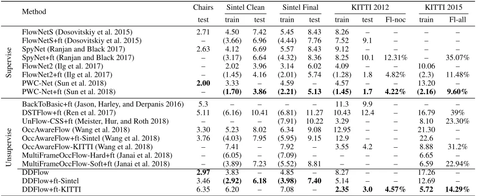
Method Chairs Sintel Clean Sintel Final KITTI 2012 KITTI 2015 test train test train test train test Fl-noc train Fl-all
Supervise
FlowNetS (Dosovitskiy et al. 2015) 2.71 4.50 7.42 5.45 8.43 8.26 – – – – FlowNetS+ft (Dosovitskiy et al. 2015) – (3.66) 6.96 (4.44) 7.76 7.52 9.1 – – – SpyNet (Ranjan and Black 2017) 2.63 4.12 6.69 5.57 8.43 9.12 – – – – SpyNet+ft (Ranjan and Black 2017) – (3.17) 6.64 (4.32) 8.36 8.25 10.1 12.31% – 35.07% FlowNet2 (Ilg et al. 2017) – 2.02 3.96 3.14 6.02 4.09 – – 10.06 – FlowNet2+ft (Ilg et al. 2017) – (1.45) 4.16 (2.01) 5.74 (1.28) 1.8 4.82% (2.3) 11.48% PWC-Net (Sun et al. 2018) 2.00 3.33 – 4.59 – 4.57 – – 13.20 – PWC-Net+ft (Sun et al. 2018) – (1.70) 3.86 (2.21) 5.13 (1.45) 1.7 4.22% (2.16) 9.60%
Unsupervise
BackToBasic+ft (Jason, Harley, and Derpanis 2016) 5.3 – – – – 11.3 9.9 – – – DSTFlow+ft (Ren et al. 2017) 5.11 (6.16) 10.41 (6.81) 11.27 10.43 12.4 – 16.79 39% UnFlow-CSS+ft (Meister, Hur, and Roth 2018) – – – (7.91) 10.22 3.29 – – 8.10 23.30% OccAwareFlow (Wang et al. 2018) 3.30 5.23 8.02 6.34 9.08 12.95 – – 21.30 – OccAwareFlow+ft-Sintel (Wang et al. 2018) 3.76 (4.03) 7.95 (5.95) 9.15 12.9 – – 22.6 – OccAwareFlow-KITTI (Wang et al. 2018) – 7.41 – 7.92 – 3.55 4.2 – 8.88 31.2% MultiFrameOccFlow-Hard+ft (Janai et al. 2018) – (6.05) – (7.09) – – – – 6.65 – MultiFrameOccFlow-Soft+ft (Janai et al. 2018) – (3.89) 7.23 (5.52) 8.81 – – – 6.59 22.94% DDFlow 2.97 3.83 – 4.85 – 8.27 – – 17.26 – DDFlow+ft-Sintel 3.46 (2.92) 6.18 (3.98) 7.40 5.14 – – 12.69 – DDFlow+ft-KITTI 6.35 6.20 – 7.08 – 2.35 3.0 4.57% 5.72 14.29%
Table 1: Comparison to state-of-the-art optical flow estimation methods. All numbers are EPE except for the last column of KITTI 2012 and KITTI 2015 test sets, where we report percentage of erroneous pixels (Fl). Missing entries (-) indicate that the results are not reported for the respective method. Parentheses mean that the training is performed on the same dataset. Bold fonts highlight the best results among supervised and unsupervised methods respectively. Note that MultiFrameOccFlow (Janai et al. 2018) utilizes multiple frames, while all other methods use only two consecutive frames.
occlusion map as an example, we first compute the reversed forward flowwˆf =wb(p+wf(p)), wherep ∈Ω. A pixel
is considered occluded if either of the following constraints is violated:
|wf+ ˆwf|2< α1(|wf|2+|wˆf|2) +α2,
p+wf(p)∈/Ω, (1)
where we setα1= 0.01,α2= 0.05 for all our experiments.
Backward occlusion maps are computed in the same way.
Photometric Loss.The photometric loss is based on the brightness constancy assumption, which measures the dif-ference between the redif-ference image and the warped target image. It is only effective for non-occluded pixels. We define a simple loss as follows:
Lp=Xψ(I1−I2w)(1−Of)/
X
(1−Of)
+Xψ(I2−I1w)(1−Ob)/
X
(1−Ob) (2)
whereψ(x) = (|x|+)q is a robust loss function,
de-notes the element-wise multiplication. During our experi-ments, we set = 0.01,q = 0.4. Our teacher model only minimizes this loss.
Loss for Occluded Pixels.The key element in unsuper-vised learning is the loss for occluded pixels. In contrast to existing loss functions relying on smoothing prior to con-strain flow estimation, our loss is purely data-driven. This enables us to directly learn from real data, and produce more accurate flow. To this end, we define our loss on pixels that are occluded in the cropped patch but non-occluded in the original image. Then, supervision is generated using predic-tions of the original image from our teacher model, which produces reliable optical flow for non-occluded pixels.
To find these pixels, we first compute a valid maskM rep-resenting the pixels that are occluded in the cropped image but non-occluded in the original image:
Mf =clip(Oef−O
p
f,0,1) (3)
Backward maskMbis computed in the same way. Then we define our loss for occluded pixels in the following,
Lo=Xψ(wpf−wef)Mf/
X
Mf
+Xψ(wpb−web)Mb/
X
Mb (4)
We use the same robust loss function ψ(x)with the same parameters defined in Eq. 2. Our student model minimizes the simple combinationLp+Lo.
Experiments
(a) Input Image 1 (b) GT Flow (c) Our Flow (d) GT Occlusion (e) Our Occlusion
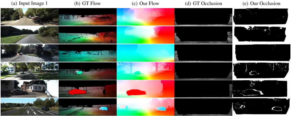
Figure 5: Example results on KITTI datasets. The first three rows are from KITTI 2012, and the last three are from KITTI 2015. Our method estimates accurate optical flow and reliable occlusion maps. Note that on KITTI datasets, the occlusion masks are sparse and only contain pixels moving out of the image boundary.
Implementation Details
Data Preprocessing. We preprocess the image pairs us-ing census transform (Zabih and Woodfill 1994), which is proved to be robust for optical flow estimation (Hafner, Demetz, and Weickert 2013). We find that this simple pro-cedure can indeed improve the performance of unsupervised optical flow estimation, which is consistent with (Meister, Hur, and Roth 2018).
Training procedure. For all our experiments, we use the same network architecture and train our model using Adam optimizer (Kingma and Ba 2014) withβ1 =0.9 and
β2=0.999. For all datasets, we set batch size as 4. For all
in-dividual experiments, we use a initial learning rate of 1e-4, and it decays half every 50k iterations. For data augmen-tation, we only use random cropping, random flipping, and random channel swapping. Thanks to the simplicity of our loss functions, there is no need to tune hyper-parameters.
Following prior work, we first pre-train DDFlow on Fly-ing Chairs. We initialize our teacher network from random, and warm it up with 200k iterations using our photometric loss without considering occlusion. Then, we add our occlu-sion detection check, and train the network with the photo-metric lossLpfor another 300k iterations. After that, we
ini-tialize the student model with the weights from our teacher model, and train both the teacher model (withLp) and the student model (withLp+Lo) together for 300k iterations. This concludes our pre-training, and the student model is used for future fine-tuning.
We use the same fine-tuning procedure for all Sintel and KITTI datasets. First, we initialize the teacher network using the pre-trained student model from Flying Chairs, and train it for 300k iterations. Then, similar to pre-training on Fly-ing Chairs, the student network is initialized with the new teacher model, and both networks are trained together for another 300k iterations. The student model is used during our evaluation.
Evaluation Metrics.We consider two widely-used met-rics to evaluate optical flow estimation and one metric of oc-clusion evaluation: average endpoint error (EPE), percent-age of erroneous pixels (Fl), harmonic averpercent-age of the pre-cision and recall (F-measure). We also report the results of EPE over non-occluded pixels (NOC) and occluded pixels (OCC) respectively. EPE is the ranking metric on MPI Sin-tel benchmark, and Fl is the ranking metric on KITTI bench-marks.
Comparison to State-of-the-art
We compare our results with state-of-the art methods in Ta-ble 1. As we can see, our approach, DDFlow, outperforms all existing unsupervised flow learning methods on all datasets. On the test set of Flying Chairs, our EPE is better than all prior results, decreasing from previous state-of-the-art 3.30 to 2.97. More importantly, simply evaluating our model only pre-trained on Flying Chairs, DDFlow achieves EPE=3.83 on Sintel Clean and EPE=4.85 on Sintel Final, which are even better than the results from state-of-the-art unsuper-vised methods (Wang et al. 2018; Janai et al. 2018) fine-tuned specifically for Sintel. This is remarkable, as it shows the great generalization capability of DDFlow.
After we finetuned DDFlow using frames from the Sin-tel training set, we achieved an EPE=7.40 on the SinSin-tel Final testing benchmark, improving the best prior result (EPE=8.81 from (Janai et al. 2018)) by a relative margin of 14.0 %. Similar improvement (from 7.23 to 6.18) is also ob-served on the Sintel Clean testing benchmark. Our model is even better than some supervised methods including (Doso-vitskiy et al. 2015) and (Ranjan and Black 2017), which are finetuned on Sintel using ground truth annotations. Fig-ure 4 shows sample DDFlow results from Sintel, comparing our optical flow estimations and occlusion masks with the ground truth.
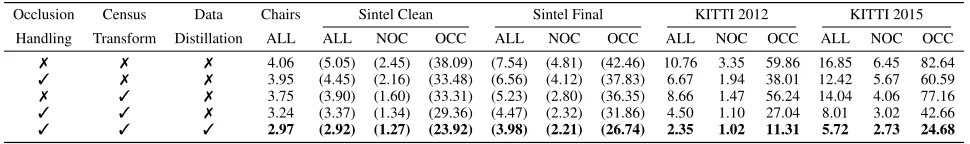
Occlusion Census Data Chairs Sintel Clean Sintel Final KITTI 2012 KITTI 2015
Handling Transform Distillation ALL ALL NOC OCC ALL NOC OCC ALL NOC OCC ALL NOC OCC
7 7 7 4.06 (5.05) (2.45) (38.09) (7.54) (4.81) (42.46) 10.76 3.35 59.86 16.85 6.45 82.64
3 7 7 3.95 (4.45) (2.16) (33.48) (6.56) (4.12) (37.83) 6.67 1.94 38.01 12.42 5.67 60.59
7 3 7 3.75 (3.90) (1.60) (33.31) (5.23) (2.80) (36.35) 8.66 1.47 56.24 14.04 4.06 77.16
3 3 7 3.24 (3.37) (1.34) (29.36) (4.47) (2.32) (31.86) 4.50 1.10 27.04 8.01 3.02 42.66
3 3 3 2.97 (2.92) (1.27) (23.92) (3.98) (2.21) (26.74) 2.35 1.02 11.31 5.72 2.73 24.68
Table 2: Ablation study. We compare the results of EPE over all pixels (ALL), non-occluded pixels (NOC) and occluded pixels (OCC) under different settings. Bold fonts highlight the best results.
Method Sintel Sintel KITTI KITTI
Clean Final 2012 2015
MODOF – 0.48 – –
OccAwareFlow-ft (0.54) (0.48) 0.95∗ 0.88∗
MultiFrameOccFlow-Soft+ft (0.49) (0.44) – 0.91∗
Ours (0.59) (0.52) 0.94∗ 0.86∗
Table 3: Comparison to state-of-the-art occlusion estimation methods.∗ marks cases where the occlusion map is sparse and only the annotated pixels are considered.
more significant. On KITTI 2012 testing set, DDFlow yields an EPE=3.0, 28.6 % lower than the best existing counterpart (EPE=4.2 from (Wang et al. 2018)). For the ranking mea-surement on KITTI 2012, we achieve Fl-noc=4.57 %, even better than the result (4.82 %) from the well-known FlowNet 2.0. For KITTI 2015, DDFlow performs particularly well. The Fl-all from DDFlow reaches 14.29%, not only better than the best unsupervised method by a large margin (37.7 % relative improvement), but also outperforming several re-cent fully supervised learning methods including (Ran-jan and Black 2017; Bailer, Varanasi, and Stricker 2017; Zweig and Wolf 2017; Xu, Ranftl, and Koltun 2017). Ex-ample results from KITTI 2012 and 2015 can be seen in Figure 5.
Occlusion Estimation
Next, we evaluate our occlusion estimation on both Sin-tel and KITTI dataset. We compare our method with MODOF(Xu, Jia, and Matsushita 2012), OccAwareFlow-ft(Wang et al. 2018), MultiFrameOccFlow-Soft+ft(Janai et al. 2018) using F-measure. Note KITTI datasets only have sparse occlusion map.
As shown in Table 3, our method achieve best occlu-sion estimation performance on Sintel Clean and Sintel Final datasets over all competing methods. On KITTI dataset, the ground truth occlusion masks only contain pixels moving out of the image boundary. However, our method will also estimate the occlusions within the image range. Under such settings, our method can achieve comparable performance.
Ablation Study
We conduct a thorough ablation analysis for different com-ponents of DDflow. We report our findings in Table 2.
Occlusion Handling. Comparing the first row and the second row, the third row and the fourth row, we can see that occlusion handling can improve the optical flow
estima-tion performance over all pixels, non-occluded pixels and occluded pixels on all datasets. It is because that brightness constancy assumption does not hold for occluded pixels.
Census Transform. Census transform can compensate for illumination changes, which is robust for optical flow estimation and has been widely used in traditional methods. Comparing the first row and the third row, the second row and the fourth row, we can see that it indeed constantly im-proves the performance on all datasets.
Data Distillation.Since brightness constancy assumption does not hold for occluded pixels and there is no ground truth flow for occluded pixels, we introduce a data distilla-tion loss to address this problem. As shown in the fourth row and the fifth row, occluded prediction can improve the performance on all datasets, especially for occluded pixels. EPE-OCC decreases from 29.36 to 23.93 (by 18.5 %) on Sintel Clean, from 31.86 to 26.74 (by 16.1 %) on Sintel Fi-nal dataset, from 27.04 to 11.31 (by 58.2 %) on KITTI 2012 and from 42.66 to 24.68 (by 42.1 %) on KITTI 2015. Such a big improvement demonstrates the effectiveness of DDFlow. Our distillation strategy works particularly well near im-age boundary, since our teacher model can distill reliable labels for these pixels. For occluded pixels elsewhere, our method is not as effective, but still produces reasonable re-sults to some extent. This is because we crop at random lo-cation for student model, which covers a large amount of occlusions. Exploring new ideas to cope with occluded pix-els at any location can be a promising research direction in the future.
Conclusion
References
Bailer, C.; Varanasi, K.; and Stricker, D. 2017. Cnn-based patch matching for optical flow with thresholded hinge em-bedding loss. InCVPR.
Bonneel, N.; Tompkin, J.; Sunkavalli, K.; Sun, D.; Paris, S.; and Pfister, H. 2015. Blind video temporal consistency.
ACM Trans. Graph.34(6):196:1–196:9.
Brox, T., and Malik, J. 2011. Large displacement optical flow: descriptor matching in variational motion estimation.
TPAMI33(3):500–513.
Brox, T.; Bruhn, A.; Papenberg, N.; and Weickert, J. 2004. High accuracy optical flow estimation based on a theory for warping. InECCV.
Butler, D. J.; Wulff, J.; Stanley, G. B.; and Black, M. J. 2012. A naturalistic open source movie for optical flow evaluation. InECCV.
Chauhan, A. K., and Krishan, P. 2013. Moving object track-ing ustrack-ing gaussian mixture model and optical flow. Interna-tional Journal of Advanced Research in Computer Science and Software Engineering3(4).
Dosovitskiy, A.; Fischer, P.; Ilg, E.; Hausser, P.; Hazirbas, C.; Golkov, V.; Van Der Smagt, P.; Cremers, D.; and Brox, T. 2015. Flownet: Learning optical flow with convolutional networks. InICCV.
Eigen, D.; Puhrsch, C.; and Fergus, R. 2014. Depth map prediction from a single image using a multi-scale deep net-work. InNIPS.
Geiger, A.; Lenz, P.; and Urtasun, R. 2012. Are we ready for autonomous driving? the kitti vision benchmark suite. In
CVPR.
Hafner, D.; Demetz, O.; and Weickert, J. 2013. Why is the census transform good for robust optic flow computation? InInternational Conference on Scale Space and Variational Methods in Computer Vision.
Hinton, G.; Vinyals, O.; and Dean, J. 2015. Distill-ing the knowledge in a neural network. arXiv preprint arXiv:1503.02531.
Horn, B. K., and Schunck, B. G. 1981. Determining optical flow.Artificial intelligence17(1-3):185–203.
Hui, T.-W.; Tang, X.; and Loy, C. C. 2018. Liteflownet: A lightweight convolutional neural network for optical flow estimation. InCVPR.
Ilg, E.; Mayer, N.; Saikia, T.; Keuper, M.; Dosovitskiy, A.; and Brox, T. 2017. Flownet 2.0: Evolution of optical flow estimation with deep networks. InCVPR.
Janai, J.; G¨uney, F.; Ranjan, A.; Black, M. J.; and Geiger, A. 2018. Unsupervised learning of multi-frame optical flow with occlusions. InECCV.
Jason, J. Y.; Harley, A. W.; and Derpanis, K. G. 2016. Back to basics: Unsupervised learning of optical flow via bright-ness constancy and motion smoothbright-ness. InECCV.
Kingma, D. P., and Ba, J. 2014. Adam: A method for stochastic optimization.arXiv preprint arXiv:1412.6980. Liu, C.; Freeman, W. T.; Adelson, E. H.; and Weiss, Y. 2008. Human-assisted motion annotation. InCVPR.
Mayer, N.; Ilg, E.; Hausser, P.; Fischer, P.; Cremers, D.; Dosovitskiy, A.; and Brox, T. 2016. A large dataset to train convolutional networks for disparity, optical flow, and scene flow estimation. InCVPR.
Meister, S.; Hur, J.; and Roth, S. 2018. UnFlow: Unsu-pervised learning of optical flow with a bidirectional census loss. InAAAI.
Menze, M., and Geiger, A. 2015. Object scene flow for autonomous vehicles. InCVPR.
Radosavovic, I.; Doll´ar, P.; Girshick, R.; Gkioxari, G.; and He, K. 2018. Data distillation: Towards omni-supervised learning.CVPR.
Ranjan, A., and Black, M. J. 2017. Optical flow estimation using a spatial pyramid network. InCVPR.
Ren, Z.; Yan, J.; Ni, B.; Liu, B.; Yang, X.; and Zha, H. 2017. Unsupervised deep learning for optical flow estimation. In
AAAI.
Revaud, J.; Weinzaepfel, P.; Harchaoui, Z.; and Schmid, C. 2015. Epicflow: Edge-preserving interpolation of correspon-dences for optical flow. InCVPR.
Simonyan, K., and Zisserman, A. 2014. Two-stream convo-lutional networks for action recognition in videos. InNIPS. Sun, D.; Yang, X.; Liu, M.-Y.; and Kautz, J. 2018. Pwc-net: Cnns for optical flow using pyramid, warping, and cost volume. InCVPR.
Sun, D.; Roth, S.; and Black, M. J. 2010. Secrets of optical flow estimation and their principles. InCVPR.
Sundaram, N.; Brox, T.; and Keutzer, K. 2010. Dense point trajectories by gpu-accelerated large displacement optical flow. InECCV.
Wang, Y.; Yang, Y.; Yang, Z.; Zhao, L.; and Xu, W. 2018. Occlusion aware unsupervised learning of optical flow. In
CVPR.
Weinzaepfel, P.; Revaud, J.; Harchaoui, Z.; and Schmid, C. 2013. Deepflow: Large displacement optical flow with deep matching. InICCV.
Xu, L.; Jia, J.; and Matsushita, Y. 2012. Motion detail pre-serving optical flow estimation. TPAMI34(9):1744–1757. Xu, J.; Ranftl, R.; and Koltun, V. 2017. Accurate Optical Flow via Direct Cost Volume Processing. InCVPR. Zabih, R., and Woodfill, J. 1994. Non-parametric local transforms for computing visual correspondence. InECCV. Zbontar, J., and LeCun, Y. 2016. Stereo matching by training a convolutional neural network to compare image patches.JMLR17(1-32):2.