The Thirty-Third AAAI Conference on Artificial Intelligence (AAAI-19)
Bootstrap Estimated Uncertainty of the
Environment Model for Model-Based Reinforcement Learning
Wenzhen Huang,
1,2Junge Zhang,
1,2Kaiqi Huang
1,2,3 1CRISE, Institute of Automation, Chinese Academy of Sciences, Beijing, China2University of Chinese Academy of Sciences, Beijing, China
3CAS Center for Excellence in Brain Science and Intelligence Technology, Beijing, China
{wenzhen.huang, jgzhang, kqhuang}@nlpr.ia.ac.cn
Abstract
Model-based reinforcement learning (RL) methods attempt to learn a dynamics model to simulate the real environment and utilize the model to make better decisions. However, the learned environment simulator often has more or less model error which would disturb making decision and reduce perfor-mance. We propose a bootstrapped model-based RL method which bootstraps the modules in each depth of the planning tree. This method can quantify the uncertainty of environ-ment model on different state-action pairs and lead the agent to explore the pairs with higher uncertainty to reduce the potential model errors. Moreover, we sample target values from their bootstrap distribution to connect the uncertain-ties at current and subsequent time-steps and introduce the prior mechanism to improve the exploration efficiency. Ex-periment results demonstrate that our method efficiently de-creases model error and outperforms TreeQN and other state-of-the-art methods on multiple Atari games.
Introduction
Model-based reinforcement learning (RL) methods learn a model of the environment from its experience. Using the internal model to simulate the environment, the agent can plan and avoid making poor decisions. However, building a perfect environment model without errors in complex do-mains is hard, and it would be harder when the transition and reward functions of the environment are stochastic. The model errors would mislead the agent and degrade its perfor-mances during the process of planning and deciding (Talvitie 2014). Some methods (Tamar et al. 2016; Silver et al. 2017; Oh, Singh, and Lee 2017; Farquhar et al. 2017) attempt to replace observation-prediction model with value-prediction model to decrease prediction error. There are also several methods trying to quantify the errors (Asadi, Misra, and Littman 2018) or make robust decisions based on the im-precise model (Racani`ere et al. 2017).
Different from above model-based methods, we attempt to actively find and reduce the potential model errors. We proposed a bootstrapped model-based RL method which can utilize bootstrap to quantify the uncertainty of predicted re-wards and Q-values on the different state-action pairs and lead the agent to explore the pairs with high uncertainty. The
Copyright c2019, Association for the Advancement of Artificial Intelligence (www.aaai.org). All rights reserved.
core idea is as follows. The method builds up multiple envi-ronment models with the identical network architectures and randomly samples different experience replays to train these models. Each learned model can be seen as a sample from the environment model’s approximate posterior. Then the agent randomly samples an environment model and utilizes it to predict and plan inT steps. For the state-action pairs with high uncertainty, the rewards or Q-values estimated by different environment models would fluctuate more greatly. As a result, they would be more likely to be predicted as large values by some models, and the pairs would be more likely to be visited. Thus, this bootstrap method can guide the agent to explore the state-action pairs which are ‘un-familiar’ for environment model and reduce the potential model errors.
We apply this idea to TreeQN (Farquhar et al. 2017), a model-based RL method which learn a value-prediction model and utilizes the model to build a look-ahead tree to plan. The transition, reward and value functions of TreeQN form the environment model, thus we would quantify the un-certainty of these functions through the bootstrap method. Considering that the model errors generally increase with the planning depth, we establish multiple environment mod-ule sets to quantify the uncertainty in different depth. Fur-thermore, we construct the look-ahead trees through sam-pling modules from each set and using them to generate the terms in different depth of the tree. Randomly gener-ated trees are utilized to select the appropriate actions, cal-culate the target values and optimize the environment model in the same way of TreeQN. As each module is trained by the re-sampled transitions, the models assembled by them can be considered as the bootstrap estimates of the environ-ment model. Thus, the target Q-values estimated based on these models reflect the uncertainties of Q-value estimation at subsequent time-steps. The uncertainties on current and subsequent time-steps can be connected when the Q-value is updated using the target Q-values at subsequent states, which can help our method to learn the uncertainty of Q-estimator faster.
architec-ture as the module but the parameters in the prior network are fixed as random initial parameter.
Experiment results show that our method outperforms TreeQN and other state-of-the-art methods in multiple do-mains. Our method can obviously decrease the reward pre-diction losses, which illustrates that the model errors are in-deed diminished. Additionally, we prove the importance of the mechanisms of sampling targets from their bootstrap dis-tribution and adding prior network through removing them respectively.
Related Work
Deep Q-Network (DQN) proposed by (Mnih et al. 2015) trains deep neural networks to estimate the action-values (or Q-values) and solves the problem that action-value function is divergent when it is approximated with neural networks. The performance of DQN is comparable to human play-ers on Atari games (Bellemare et al. 2013), which means that reinforcement learning (RL) approaches can be applied to complex, high-dimensional environments. Many varia-tions of DQN are proposed to solve the shortcomings in DQN or adapt it to specific environments, like (van Hasselt, Guez, and Silver 2016; Wang et al. 2016; Schaul et al. 2015; Osband et al. 2016; Fortunato et al. 2017; Bellemare, Dab-ney, and Munos 2017; Hausknecht and Stone 2015).
Different from the above free methods, model-based RL methods learn an environment model and plan with the help of this model. Dyna-Q (Sutton 1990) learns an observation-prediction model and uses the samples gen-erated by the environment model and obtained from the real environment for Q-learning. Imagination-augmented agents (Weber et al. 2017) use the environment model to generate rollout trajectories and aggregate them to improve policies through RNN. This kind of environment models can also be used to improve exploration (Oh et al. 2015; Chiappa et al. 2017).
As the observation-prediction model is difficult to build for the environments with large observation space, some en-vironment models are learned in the abstract state space and predict future rewards or values instead of future observa-tions. Predictrons (Silver et al. 2017) learn an abstract en-vironment model to predict rewards and values over multi-ple planning depths. However, it can only be used for policy evaluation. Value Prediction Networks (VPNs) (Oh, Singh, and Lee 2017) is on the basis of the similar idea but uses the abstract model to construct a look-ahead tree and aggre-gate the predicted rewards and values to estimate Q-values. And these Q-values are used to calculate targets and choose actions. Like VPNs, TreeQN (Farquhar et al. 2017) also builds a tree for planning, but it replaces convolutional tran-sition functions with full-connnected ones to simplify train-ing. What’s more, the environment model is embedded in the planning algorithm to optimize.
However, it’s hard to learn an accurate model for the com-plex environments. Imagination-augmented agents attempt to make robust decisions based on the imprecise model. VINs, Predictrons, VPNs and TreeQN replace observation-prediction models with value-observation-prediction models to reduce
model error. Different from them, our method actively seeks and reduces the potential model errors.
Background
Deep Q-Network (DQN)
Reinforcement learning (RL) addresses the problem that an agent learns to interact with the environment to maximize the return. At each time step t, the agent receives an ob-servation st from the environment, and responds with an
action at selected from the set of all possible actions A.
Then the agent receives a reward rtand the next
observa-tion st+1. These interactions would continue until the
en-vironment arrives some terminal states. This process can be viewed as a Markov Decision Process, which is de-fined by the tuple(S,A,T,R), whereSis the state space,
T =P(st+1=s0|st=s, at=a)is the transition function,
andR=P(rt =r|st=s, at=a)is the reward function.
The agent’s goal is finding a good policyπto maximize the return, which is defined as the discounted sum of future re-wards starting from time stept,Rt=
Pinf
k=0γ
kr
t+k, where
γ∈(0,1]is the discount factor.
In value-based reinforcement learning, the agent learns to estimate the expected return starting from given statestand
actionat, denoted as Q-valueQ(st, at). DQN uses a
convo-lutional neural network to estimate Q-values. At time step
t, the agent selects an action according to the estimated Q-valuesQ(st,·)underε-greedy scheme. The neural network
is optimized by minimizing the Q-value loss,
LQ =
ˆ
Rt−Q(st, at;θ)
2
, (1)
whereRˆt =rt+γmaxaQ(st+1, a;θ−)is the approxima-tion of the return, and θ− are target network parameters. Specially, in then-step DQN (Mnih et al. 2016),Rˆtis set
asPn−1
k=0γ
kr
t+k+γnmaxaQ(st+n, a;θ−)to improve the
stability and speed of the algorithm.
Bootstrapped DQN
Efficient exploration is an important challenge in reinforce-ment learning field. The authors of (Osband et al. 2016) be-lieve that an available solution is quantifying uncertainty in value estimates and encouraging agent to explore the state-action pairs with high potential benefits. They pro-pose bootstrapped DQN which combines DQN with a non-parametric bootstrap method and can quantify uncertainty over Q-values. In details, bootstrapped DQN has K ∈ N
Q-value functionsQk(s, a;θ), k= 1,2, . . . , Kwhich share
the same network except the last layer. The target network has the same architecture so that Q-value functions can be trained against their respective target functions. In each episode, a Q-value function Qk(s, a;θ) is randomly
sam-pled and guides the agent to select optimal actions estimated by itself. Before each replay(s, a, r, s0)is added into the re-play buffer, it is tagged with an independent Bernoulli mask
w1, w2, . . . , wK ∼ Ber(p), wherep is the probability of
can be trained on the replay. In this way, each Q-value func-tion is trained by different samples of the total replays and can be seen as an approximate bootstrap sample.
TreeQN
TreeQN (Farquhar et al. 2017) is a model-based RL method which uses a recursive architecture for tree planning. TreeQN contains five main modules: The first module is en-coder function z0|t = encode(st;θen), which embeds the
observed statest to the state representation z0|t. The
sec-ond one is transition functionzd+1|t=t(zd|t, ai;θt), which
generates the next state representationzd+1|tfor the action
ad ∈ Ain statezd|t.zd|tdenotes the predicted state
repre-sentation at timetafterdinternal simulated transitions. The third one is reward functionr(zd|t, ai;θr), which predicts
the reward for state-action pair(zd|t, ai). The fourth one is
value functionv(zd|t;θv), which estimates the value of the
state representationv(zd|t). The last one is backup function
b(x), which mixes the intermediate values and rewards into the final estimate ofQ(st, ai).
TreeQN utilizes the transition and reward functions re-cursively to set up aD-depth tree containing the predicted state representations and rewards for all possible action se-quences{(a1, a2, . . . , aD)|ad∈ A}, whereDis predefined
planning depth. Then TreeQN uses the value function and the predicted rewards to mix the returns along each path in the tree:
Q(zd|t, ai) =r(zd|t, ai) +γV(zd+1|t)
V(zd|t) =
(
v(zai
d|t), d=D
(1−λ)v(zai
d|t) +λb(Q(z ai
d|t, aj)), d < D
In this way, TreeQN refines its Q-value estimation via inter-nal transition, reward, and value functions.
It is worth noted that the architecture of TreeQN com-bining all the five modules is differentiable. Thus it can be trained with any deep RL algorithm by viewing the whole planning network as Q-network. To train efficiently the in-ternal environment model, a reward-prediction loss Lr is
added to the Q-value loss. The reward-prediction loss Lr
is defined as an L2 loss between the predicted rewardrd|t
for the actual action sequence, and the true obtained reward
rt+d:
Lr= D−1 X
d=0
(rd|t−rt+d)2.
ATreeC (Farquhar et al. 2017) is proposed as an actor-critic variant of TreeQN, which is implemented by convert-ing the Q-valuesQ(s, a)to the policyπ(s, a)with a softmax layer.
Approach
Motivation
Model-based reinforcement learning methods focus on learning a dynamics model to simulate the environment and planning or making better decisions based on the simula-tion results. These methods have good interpret-ability of
the obtained policies and can be effective in some domains. But it is often difficult to build a highly accurate environ-ment model in complex domains, especially when the transi-tion and reward functransi-tions are stochastic. During the process of planning and deciding, the model errors would mislead the agent and degrade its performance (Talvitie 2014). The model errors still exist whether the model’s prediction is the next observation or the value of next state. There are some methods attempting to quantify the errors (Asadi, Misra, and Littman 2018) or make robust decisions based on the impre-cise model (Racani`ere et al. 2017).
Different from them, we attempt to actively find and re-duce the potential model errors. The bootstrap is a data-based simulation method for assigning a level of confidence on the statistics estimates (Efron and Tibshirani 1994). We consider utilizing bootstrap to quantify the uncertainty of en-vironment model’s predictions on the different state-action pairs and guide the agent to explore the pairs with high un-certainty. As a result, the uncertainty decreases with the sam-pling number of these pairs increasing.
Bootstrapped Model-Based RL
In this section, we first take a brief look at the idea of our bootstrapped model-based RL method, and then we would introduce it in details.
The core idea of bootstrap is to “approximate a population distribution by a sample distribution” (Efron and Tibshirani 1994; Osband et al. 2016). For a data setDand an estima-torϕ, the bootstrap sampleϕ(De)is generated by taking the estimatorϕon the data set De which is sampled uniformly with replacement fromDand has the same size asD.
Our goal is quantifying the uncertainty of environment model through the bootstrap. In this problem, the data set is the total experience transitions and the estimator is the en-vironment model. Thus, we build up multiple enen-vironment models and randomly sample the experience transitions to train these models. In this way, each model can be consid-ered as an approximate bootstrap sample. When the agent needs environment model to predict and plan, we randomly sample an environment model, and the agent will utilize it in the episode (orT steps).
For the state-action pairs which are less visited or have more stochastic reward and transition functions, the learned environment models have more uncertainty on these pairs and the values estimated by different environment models would fluctuate more greatly. As a result, the rewards or Q-values on the pairs are more likely to be estimated as large value by some environment models and the pairs are more likely to be visited. Therefore, this bootstrap method can re-duce model error by guiding the agent’s exploration.
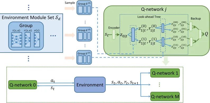
Now, we apply this idea to TreeQN which embeds the environment model in its Q-network through constructing a look-ahead tree and aggregating the predicted rewards and values to estimate Q-values. The overall framework is shown in Figure 1. TreeQN contains five main modules: encoder functionencode(st;θen), action-dependent
transi-tion functransi-tion t(zd|t, ai;θt), action-dependent reward
Environment Module Set 𝒮𝑑
…
𝑡(𝑠, 𝑎) 𝑟(𝑠, 𝑎) 𝑣(𝑠)Group
Environment Q-network 0 𝑎𝑠t
𝑡
𝑠𝑡, 𝑎𝑡, 𝑟𝑡, 𝑠t+1
…
Q-network 1
Q-network M Q-network 𝑗
𝑠𝑡 𝑧0|𝑡
𝑧1|𝑡(1), 𝑟1|𝑡(1)
Encoder
𝑄
Backup
…
…
Sample Group 𝑘(0)Group 𝑘(𝐷)
…
Group 𝑘(𝑑)
…
𝑧1|𝑡(0), 𝑟1|𝑡(0)
𝑧2|𝑡 (00)
, 𝑟2|𝑡 (00)
𝑧2|𝑡(01), 𝑟2|𝑡(01)
𝑧2|𝑡 (10)
, 𝑟2|𝑡 (10)
𝑧2|𝑡 (11)
, 𝑟2|𝑡 (11) Look-ahead Tree
Figure 1: Overview of our bootstrapped model-based reinforcement learning method. To quantify uncertainty in model esti-mation, we establishD+ 1environment module sets. Each set containsKgroups of modules, each of which is composed of transition modulet(s, a), reward moduler(s, a)and value modulev(s). EachTsteps, we randomly sample a group from each set and utilize them to build the look-ahead tree. The tree is embedded in the Q-network to guide the action selections. At every update iteration, we buildM different Q-networks, and their parameters are updated by minimizing the n-step Q-value loss and the reward prediction loss on the experience tuples(st, at, rt, st+1).
functionb(x). Among them, the transition, reward and value functions form the environment model, thus we would quan-tify the uncertainty of these functions through the bootstrap method.
Due to the fact that the model errors accumulate with the times of intermediate transiting, the uncertainty would also increase with the depth dof the planning tree. In ad-dition, in the stochastic environment the uncertainty of fu-ture statesst0and rewardsrt0also increase with the distance from current time to timet0. Therefore, we establishD+ 1 environment module sets to quantify the uncertainty of dif-ferent planning depth. In particular, thed-th set is built to quantify the uncertainty of rewards r(zd−1|t, ai) and
val-ues v(zd−1|t) predicted on the state representation zd−1|t.
All modules except encoder function and backup function use different parameter for different planning depth, like
t(zd|t, ai) =t(zd|t, ai; (θt)d).
Each environment module setSd containsK groups of
modules. Each group Gd
k contains independent transition
module td
k(s, a; (θt)dk), reward module rdk(s, a; (θr)dk) and
value modulevd
k(s; (θv)dk). The modules of each group have
the same network architecture but are randomly initialized with different parameters. As the environment model is also used to compute the target values, we establish anotherD+1 environment module setsSd−for target network.
At the beginning of eachT steps, we randomly select a groupgd
kfrom the setSdfor each depthd∈ {1,2, . . . , D+
1}. Then we build the look-ahead tree to plan and decide in the similar way of TreeQN. The predictions zd,rd and
vd in each depth of the tree is predicted by the functions
t(zd|t, ai; (θt)dk),r(zd|t, ai; (θr)dk)andv(zd|t; (θv)dk)in the
sampled groupgd k.
At every update iteration, we randomly sampleMgroups
gd
km from the set Sd for each depth with replacement. Following the method described above, we can build M
look-ahead trees and them0-th one is build by the groups
gd
km0, d = 1,2, . . . , D+ 1. Then we use these trees to estimate the Q-valuesQm(st, at)and rewardsrdm|t,
respec-tively. We also generateM look-ahead trees through sam-pling from the target module sets Sd− and utilize them to estimate target values Q−m(st, at). Then we update the
pa-rameters of the groups sampled fromSdby minimizing the
n-step Q-value loss and the reward prediction loss on the ex-perience transitions:
Ltotal=Lnstep−Q+Lr
=
M
X
m=1
"
( ˆRmt −Qm(st, at))2+ D−1
X
d=0
(rdm|t−rt+d)2
#
,
whereRˆm
t is set as
Pn−1
j=0γ
jr
t+j+γnmaxaQ−m(st+n, a).
The modules’ parameters in target modules setsSd−are up-dated by copying the ones inSdeveryTtarget steps. At the
same time, the encoder module in the target network would be updated.
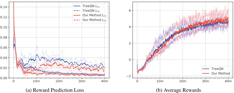
time-(a) Reward Prediction Loss (b) Average Rewards
Figure 2: Results for Box Pusing. The x-axis corresponds to time-step. The y-axes in two figures correspond to average reward over 100 episodes and average reward prediction loss over800,000time-steps respectively.Lrdmeans the reward prediction
loss in thed-th planning depth. The results of five repeated experiments are plotted faintly, while the mean of them is plotted in bold.
steps. When the Q-value is updated using the target Q-values at subsequent states, the uncertainties of Q-value estimation on current state and the ones on subsequent states can be connected. Thus, we expect that our method can propagate the uncertainty across multiple time-steps and learn the un-certainty of Q-estimator faster.
To improve the exploration efficiency, we introduce prior mechanism (Osband and Van Roy 2017; Osband, Aslanides, and Cassirer 2018), adding a frozen random prior network, to our bootstrapped model-based RL method. We add each modulef(x;θ)in total modules sets with a networkp(x;θ) which has the same architecture asf(x;θ)but parametersθ
are fixed as random initial parameter. And then the output of each modulef(x;θ)is replaced byf(x;θ) +λpp(x;θ),
whereλp∈R+is the prior scale.
Experiments
In this section, We evaluate our method in a box-pushing environment (Farquhar et al. 2017) and nine complex Atari environments (Bellemare et al. 2013). The main goals of the experiments are as follows. The first one is to confirm whether our method can decrease model errors. The sec-ond one is to determine whether our method outperforms TreeQN and other state-of-the-art methods. The last one is to verifying the rationality of bootstrapping the modules and analyze the influence of the prior mechanism and the ap-proach of calculating target values to our method.
Experiment Setting
Environment The nine complex Atari environments are Alien, Amidar, Crazy Climber, Enduro, Frostbite, Krull, Ms. Pacman, Q*Bert and Seaquest while the frameskip is set to 10. These environments are also used to evaluate VPN or TreeQN in (Oh, Singh, and Lee 2017; Farquhar et al. 2017).
The environment of “Box Pushing” is proposed by (Far-quhar et al. 2017). At the beginning of each episode, the agent, 12 boxes, 5 goals and 6 obstacles are randomly placed on the center 6 ×6 tiles of an 8×8 grid. The obstacles are passable, but they would generate a penalty if the agent or boxes are moved onto them. The agent should push the boxes into arbitrary goal in as few steps as possible while avoiding itself and boxes moving on the obstacles or leaving the grid. The episode would terminate if the agent leaves the grid, no box exists on the grid or time runs out. More details can be seen in the original paper (Farquhar et al. 2017).
Network Architecture The modules of TreeQN mostly remain their original architecture, so we only give a brief description. Encoder function is a simple CNN, consisting of two convolutional layers and a fully-connected layer. Re-ward function consists of two fully-connected layers, and the number of hidden and output units are 64 and|A| respec-tively, where |A|is the size of action space. The i-th out-put of last layer corresponds to the reward predicted for the
i-th action. Value function consists of one fully-connected layer. Transition function is composed of a shared action-independent layer and an action-dependent layer. The state representations embedded by encoder function or predicted by transition function are L2 normalized to ensure the sta-bility of transition function. Backup function is the standard maxfunction. All nonlinear activation is set to rectified lin-ear unit.
Hyperparameters Our algorithm is based on syn-chronous n-step DQN 1, the synchronous variant of asyn-chronous n-step DQN (Mnih et al. 2016) which has equal performance but makes effective use of GPUs.tmax inn
-step DQN is set to 5 and the number of threads is set to 16. The target network is updated for each 10,000 steps.
1
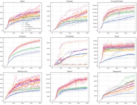
Figure 3: Learning curves on Atari games. The x-axis and y-axis correspond to step and average reward over 100 episodes, where one step is equal to 10 atomic Atari time-steps. The results of five repeated experiments are plotted faintly, while the mean of them is plotted in bold.
ε-greedy exploration decays linearly from 1.0 to 0.0 over the first 4 million steps. Owing to frameskipping, one step is equal to atomic Atari timesteps. We use RMSProp opti-mizer (Tieleman and Hinton 2012), and the learning ratelr, the decay ofαandin it are 0.0001, 0.99 and 0.00001.
The hyper-parameters in TreeQN keep identical to orig-inal paper. The weight of reward prediction loss is set to 1.0. The balance factorλis set to0.8. And we only test our method in the case of planning depthD= 2.
Our method has several more hyper-parameters. We build upK= 3groups of modules in each set. EveryT = 10,000 steps, we randomly select D + 1 = 3 module groups to build look-ahead tree. Then we sample M = 2 different groups from each set when we optimize the network. For the domains of Atari and Box Pushing, the prior scaleλpis
set to1.0and0.1, respectively.
Box Pushing
In this environment, we only compare our method with TreeQN in two planning depth. We select the same
evalu-ation mechanism as (Oh, Singh, and Lee 2017; Farquhar et al. 2017), that is, repeating the experiment five times with different random seeds and recording the average rewardRit
over 100 episodes every80,000time-steps. The results are shown in Fig. 2a and Fig. 2b respectively.
From Fig. 2a, we observe that the prediction loss increases with the depth. Thus quantifying the uncertainties of differ-ent depth separately is a reasonable choice. The losses of our method are obviously smaller than the ones of TreeQN, which means that our method can actually improve the ac-curacy of environment model.
Comparing the learning curves of two methods in Fig. 2b, our method is only sightly superior to TreeQN. One expla-nation could be that this environment is relatively simple, so the improvement of model accuracy has less impact on the final performance.
Atari
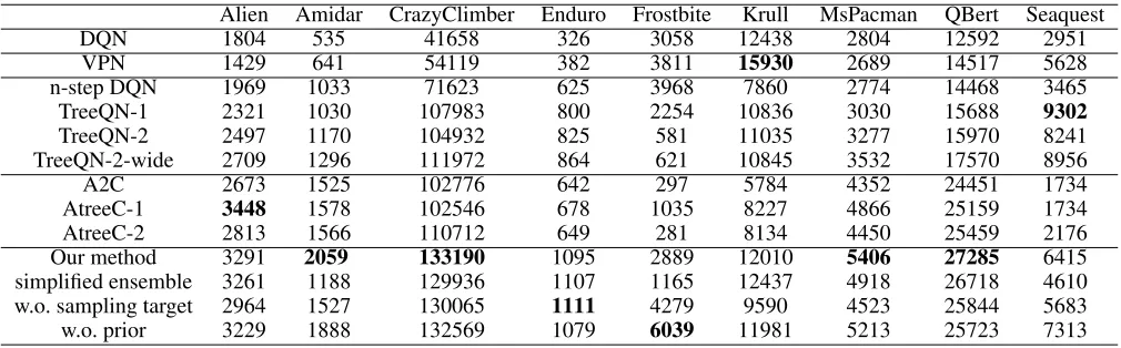
evalua-Table 1: Performance on Atari games. Each number represents the best mean score throughout training.
Alien Amidar CrazyClimber Enduro Frostbite Krull MsPacman QBert Seaquest
DQN 1804 535 41658 326 3058 12438 2804 12592 2951
VPN 1429 641 54119 382 3811 15930 2689 14517 5628
n-step DQN 1969 1033 71623 625 3968 7860 2774 14468 3465
TreeQN-1 2321 1030 107983 800 2254 10836 3030 15688 9302
TreeQN-2 2497 1170 104932 825 581 11035 3277 15970 8241
TreeQN-2-wide 2709 1296 111972 864 621 10845 3532 17570 8956
A2C 2673 1525 102776 642 297 5784 4352 24451 1734
AtreeC-1 3448 1578 102546 678 1035 8227 4866 25159 1734
AtreeC-2 2813 1566 110712 649 281 8134 4450 25459 2176
Our method 3291 2059 133190 1095 2889 12010 5406 27285 6415
simplified ensemble 3261 1188 129936 1107 1165 12437 4918 26718 4610
w.o. sampling target 2964 1527 130065 1111 4279 9590 4523 25844 5683
w.o. prior 3229 1888 132569 1079 6039 11981 5213 25723 7313
tion mechanism mentioned above to draw learning curves. Like (Oh, Singh, and Lee 2017; Farquhar et al. 2017), we calculate the mean of average rewards in the same time-steps, Rt = 15
P5
i=1R
i
t and select the best mean value
maxtRtof each game as the performance on the game.
Table 1 shows the results on nine Atari games.
TreeQN-dand ATreeC-dmeans the methods’ planning depth isd. TreeQN-2-wide means a wide version of TreeQN which doubles the size of the embedding dimension (1024 instead of 512) and roughly has the same number of parameters as the entire model of us. Our method outperforms TreeQN baseline on 8 out of 9 Atari games, especially on Alien, Ami-dar, Crazy Climber, Ms. Pacman and Q*Bert. Compared with other state-of-the-art methods, our method still outper-forms each of them on more than 7 games. We also find that TreeQN-2-wide is slightly superior to TreeQN-2, but its performance is weaker than our method except on Seaquest. Thus, the performance boost of our method cannot merely be attributed to the increase of the number of parameters.
Fig. 3 shows learning curves of DQN, TreeQN-2 and our method. Our method learned significantly faster than TreeQN on Amidar, Crazy Climber, Enduro, MS. Pacman and Q*Bert. It is noteworthy that the learning curves of TreeQN and our method are similar on all games in the first 4 million steps. At this stage, selecting actions is affected by theε-greedy strategy. After that, it depends entirely on our bootstrap method and the results begin to increase rapidly on most games. This phenomenon suggests that our exploration strategy is better for model-based RL method thanε-greedy strategy.
To verifying the rationality of bootstrapping the modules at each depth, we test a simplified ensemble approach, boot-strapping the entire TreeQN. This method is weaker than our method except on Krull. And on Krull, the performances of two method are roughly equal. One explanation could be that our method can be seen as an ensemble ofKDmodels rather
thanK models. More models mean higher performances. But for some games,Kmodels are enough.
To weigh the influence of sampling target values from their bootstrap distribution, we directly select the groups which have the same index as the groups sampled for the
online network. In other word, each module would have a fixed target module for itself as the way in (Osband et al. 2016). After replacement, the performances on 6 out of 9 games are severely decreased. It suggests that our bootstrap approach is well suited for model-based RL methods.
In addition, we also test to remove the prior mecha-nism from our method. Without this mechamecha-nism, the per-formances are obviously degraded on the games of Ami-dar, Q*Bert and Ms. Pacman, and are improved on Frostbite and Seaquest while the ones on the remaining games basi-cally keep unchanged. Comparing the learning curves of the methods with and without the mechanism, we observe that the latter one is more unstable, especially on Amidar and Crazy Climber. One explanation of these phenomena could be that the prior mechanism encourages the agent to explore the state-action pairs rarely visited. Thus, it can help the al-gorithm to escape the local optimum and improve the stabil-ity. However, it also increases the uncertainty of the predic-tions on the rare state-action pairs, which reduces the exploit efficiency on some games.
Conclusion
Acknowledgments
This work is funded by the National Key Research and Development Program of China (Grant 2016YFB1001004), the National Natural Science Foundation of China (Grant 61876181, Grant 61721004 and Grant 61403383) and the Projects of Chinese Academy of Sciences (Grant QYZDB-SSW-JSC006 and Grant 173211KYSB20160008).
References
Asadi, K.; Misra, D.; and Littman, M. L. 2018. Lipschitz continuity in model-based reinforcement learning. arXiv preprint arXiv:1804.07193.
Bellemare, M. G.; Naddaf, Y.; Veness, J.; and Bowling, M. 2013. The arcade learning environment: An evaluation plat-form for general agents. Journal of Artificial Intelligence
Research47:253–279.
Bellemare, M. G.; Dabney, W.; and Munos, R. 2017. A distributional perspective on reinforcement learning. In
In-ternational Conference on Machine Learning, 449–458.
Chiappa, S.; Racaniere, S.; Wierstra, D.; and Mohamed, S. 2017. Recurrent environment simulators. arXiv preprint
arXiv:1704.02254.
Efron, B., and Tibshirani, R. J. 1994.An introduction to the bootstrap. CRC press.
Farquhar, G.; Rockt¨aschel, T.; Igl, M.; and Whiteson, S. 2017. Treeqn and atreec: Differentiable tree plan-ning for deep reinforcement learplan-ning. arXiv preprint
arXiv:1710.11417.
Fortunato, M.; Azar, M. G.; Piot, B.; Menick, J.; Osband, I.; Graves, A.; Mnih, V.; Munos, R.; Hassabis, D.; Pietquin, O.; et al. 2017. Noisy networks for exploration. arXiv preprint
arXiv:1706.10295.
Hausknecht, M., and Stone, P. 2015. Deep recurrent q-learning for partially observable mdps. In2015 AAAI Fall
Symposium Series.
Mnih, V.; Kavukcuoglu, K.; Silver, D.; Rusu, A. A.; Ve-ness, J.; Bellemare, M. G.; Graves, A.; Riedmiller, M.; Fidjeland, A. K.; Ostrovski, G.; et al. 2015. Human-level control through deep reinforcement learning. Nature 518(7540):529.
Mnih, V.; Badia, A. P.; Mirza, M.; Graves, A.; Lillicrap, T.; Harley, T.; Silver, D.; and Kavukcuoglu, K. 2016. Asyn-chronous methods for deep reinforcement learning. In
In-ternational conference on machine learning, 1928–1937.
Oh, J.; Guo, X.; Lee, H.; Lewis, R. L.; and Singh, S. 2015. Action-conditional video prediction using deep networks in atari games. InAdvances in neural information processing
systems, 2863–2871.
Oh, J.; Singh, S.; and Lee, H. 2017. Value prediction net-work. InAdvances in Neural Information Processing Sys-tems, 6118–6128.
Osband, I., and Van Roy, B. 2017. Why is posterior sam-pling better than optimism for reinforcement learning? In
In-ternational Conference on Machine Learning, 2701–2710.
Osband, I.; Aslanides, J.; and Cassirer, A. 2018. Random-ized prior functions for deep reinforcement learning. arXiv preprint arXiv:1806.03335.
Osband, I.; Blundell, C.; Pritzel, A.; and Van Roy, B. 2016. Deep exploration via bootstrapped dqn. InAdvances in neu-ral information processing systems, 4026–4034.
Racani`ere, S.; Weber, T.; Reichert, D.; Buesing, L.; Guez, A.; Rezende, D. J.; Badia, A. P.; Vinyals, O.; Heess, N.; Li, Y.; et al. 2017. Imagination-augmented agents for deep re-inforcement learning. In Advances in Neural Information
Processing Systems, 5690–5701.
Schaul, T.; Quan, J.; Antonoglou, I.; and Silver, D. 2015. Prioritized experience replay. arXiv preprint
arXiv:1511.05952.
Silver, D.; Hasselt, H.; Hessel, M.; Schaul, T.; Guez, A.; Harley, T.; Dulac-Arnold, G.; Reichert, D.; Rabinowitz, N.; Barreto, A.; et al. 2017. The predictron: End-to-end learn-ing and plannlearn-ing. InInternational Conference on Machine
Learning, 3191–3199.
Sutton, R. S. 1990. Integrated architectures for learn-ing, plannlearn-ing, and reacting based on approximating dynamic programming. InMachine Learning Proceedings 1990. El-sevier. 216–224.
Talvitie, E. 2014. Model regularization for stable sample rollouts. InUAI, 780–789.
Tamar, A.; Wu, Y.; Thomas, G.; Levine, S.; and Abbeel, P. 2016. Value iteration networks. InAdvances in Neural
In-formation Processing Systems, 2154–2162.
Tieleman, T., and Hinton, G. 2012. Divide the gradient by a running average of its recent magnitude. coursera: Neural networks for machine learning. Technical report, Technical Report. Available online: https://zh. coursera. org/learn/neuralnetworks/lecture/YQHki/rmsprop-divide-the-gradient-by-a-running-average-of-its-recent-magnitude (accessed on 21 April 2017).
van Hasselt, H.; Guez, A.; and Silver, D. 2016. Deep re-inforcement learning with double q-learning. In Thirtieth AAAI Conference on Artificial Intelligence.
Wang, Z.; Schaul, T.; Hessel, M.; Hasselt, H.; Lanctot, M.; and Freitas, N. 2016. Dueling network architectures for deep reinforcement learning. In International Conference
on Machine Learning, 1995–2003.