Joint Label Inference in Networks
Deepayan Chakrabarti [email protected]
IROM, McCombs School of Business, University of Texas, Austin∗
Stanislav Funiak [email protected]
Cerebras Systems∗
Jonathan Chang [email protected]
Health Coda∗
Sofus A. Macskassy [email protected]
Branch Metrics∗
Editor:Edo Airoldi
Abstract
We consider the problem of inferring node labels in a partially labeled graph where each
node in the graph has multiple label types and each label type has a large number of
possible labels. Our primary example, and the focus of this paper, is the joint inference of label types such as hometown, current city, and employers for people connected by a social network; by predicting these user profile fields, the network can provide a better experience to its users. Existing approaches such as Label Propagation (Zhu et al., 2003)
fail to consider interactions between the label types. Our proposed method, called
Edge-Explain, explicitly models these interactions, while still allowing scalable inference under
a distributed message-passing architecture. On a large subset of the Facebook social
net-work, collected in a previous study (Chakrabarti et al., 2014),EdgeExplainoutperforms
label propagation for several label types, with lifts of up to 120% for recall@1 and 60% for recall@3.
Keywords: label inference, graphs, social networks, variational methods, label propaga-tion
1. Introduction
The most common classification setting assumes the presence of independent and identically distributed training examples, and attempts prediction on independent test instances drawn from the same distribution. However, the case of dependent examples has drawn much interest as well. This is particularly the case for networks where the nodes comprise the training/testing instances, and the edges between them imply dependence.
Consider the problem of inferring the labels of nodes in a network. For example, given a network of sports-related blogs connected by hyperlinks, we may want to know which blogs discuss baseball, or football, or hockey. The training data consists of known labels for a subset of blogs. The goal is to infer the labels of the remaining blogs. While the content of the blogs can be useful, the hyperlinks between blogs are clearly informative: we expect blogs to link primarily to other blogs discussing the same sport. This is a network label
∗. This research was done while the authors were employees at Facebook, Inc.
c
current city=C Node
u
hometown=H current city=C’hometown=H
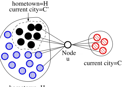
Figure 1: An example graph ofu and her friends: The hometown friends ofucoincidentally contain a subset with current city C0. This swamps the group from u’s actual current cityC, causing label propagation to inferC0foru. However, our proposed model (called EdgeExplain) correctly explains all friendships by setting the
hometown to beH and current city to be C.
inference problem with only one label type (sport) and only a few labels (baseball, football, and hockey). The question we ask is: how can we infer missing labels of multiple types, where each label type can be high-dimensional and the different types can be correlated?
The concrete problem considered in this paper is that of inferring multiple fields such as the hometowns, current cities, and employers of users of a social network, where users often only partially fill in their profile, if at all. Here, each user is associated with one label of eachtype (such as hometown, employer, etc.), and the set of possible labels for each type is very high-dimensional. Inference of such label types is important for many ranking and relevance applications. By predicting the profile fields, the social network can make better friend recommendations or show more relevant content. Consequently, accurate predictions can greatly improve the user experience. We show that this inference problem cannot be split up into separate problems, one for each label type, without loss of accuracy. Knowledge of one label type influences inferences regarding the other types. Thus, thisjoint inference
problem presents interesting opportunities for modeling and optimization.
A standard method of label inference is label propagation (Zhu and Ghahramani, 2002; Zhu et al., 2003), which tries to set the label probabilities of nodes so that friends have similar probabilities. This is based on the idea of homophily, that is, the more two nodes have in common, the more likely they are to connect (McPherson et al., 2001). However, label propagation assumes only a single category of relationships. It therefore fails to address the complexity of edge formation in networks, where nodes have different reasons to link to each other. As an example, consider the snapshot of a social network in Figure 1, where we want to predict the hometown and current city of nodeu, given what we know aboutu and
of u are from her hometown H, then inferences for current city will be dominated by the most common current city among her hometown friends (say,C0) and not friends from her actual current city C; indeed, the same will happen for all other label types as well.
Our proposed method, named EdgeExplain, approaches the problem from a different
viewpoint, using the following intuition: Two people form an edge in a social network because they share the same label for one or more label types (e.g., both went to the same college). Using this intuition, we can go beyond standard label propagation in the following way: instead of taking the graph as given, and modeling labels as items that propagate over this graph, we consider the labels as factors that can explain the observed graph structure. For example, the inferences for u made by label propagation leave u’s edges from C completely unexplained. Our proposed method rectifies this, by trying to infer node labels such that for each edge u ∼v, we can explain the existence of the edge in terms of a shared label — u and v are friends from the same hometown, or college, or the like. While we are primarily interested in inferring labels, we note that the inferred reason for each edge can be useful by itself. For example, if a new node u joins a network and forms and edge with v, and we can infer that the reason is a shared college, we can recommend other college friends of v as possible new edges foru.
We note that a seemingly simple alternative solution—cluster the graph and then prop-agate the most common labels within a cluster—is in fact quite problematic. The clustering must also be complex enough to allow many overlapping clusters. This is an active area of research (Xie et al., 2013), but it still entails a significant computational burden. In addition, any clustering based solely on the graph structure ignores labels already available from user profiles, which clearly carry crucial information. A clustering method that tries to use these labels must deal with incomplete and missing labels, significantly increasing its complexity. Instead, our method will be able to operate only on dyads, without having to infer the higher-level clusters themselves. Social network cluster sizes must display wide variation (e.g., the cluster for users living in New York city versus those in small rural areas), and it is unclear if current network community detection algorithms offer good performance across the entire range of community sizes (Leskovec et al., 2010). Hence, we believe that clustering does not readily lend itself to a solution for our problem.
This paper tackles the following five questions.
How can “explaining links” be codified in a model? We propose a probabilistic model,
called EdgeExplain, for the social network given the labels of all nodes in the network.
The model has two key properties. First, the presence or absence of a link is conditionally independent of all other nodes and edges given the labels of the two endpoints of the link. This enables distributed computation for inference, which is useful for large networks. Second, labels corresponding to all the label types are jointly considered in the model.
How can inference be performed efficiently on large networks? The model likelihood function
infor-mation, i.e., when the labels of most neighbors of a node are known with relatively high certainty. This leads to our final hybrid method that combines the two approaches.
How do the model parameters affect accuracy vis-a-vis label propagation? We present an
analysis of EdgeExplain that specifies the conditions under which label propagation will
be particularly inaccurate. The quality of predictions of label propagation for a user u is shown to depend on three factors: (a) the degree to which any one label type is the preferred “reason” for forming friendships as compared to the other label types, (b) the degree to which any one label dominates among all labels of a particular type, and (c) the number of friends of a useru.
How well does it work in practice? Our iterative methods for inferring labels can be
eas-ily implemented in large-scale message-passing architectures. We empirically demonstrate their scalability on a large subset of the Facebook social network (Chakrabarti et al., 2014) and a 5 million node sample of the Google+ network (Gong et al., 2012), using publicly available user profiles and friendships. On Facebook, EdgeExplain significantly
outper-forms label propagation for several label types, with lifts of up to 120% for recall@1 and 60% for recall@3. On the Google+ sample, which exhibits extreme sparsity of labels, all algorithms are roughly equal. We also present empirical results on a movie network, where
EdgeExplainoutperforms label propagation as well as other competing methods (Zheleva
and Getoor, 2009; Yin et al., 2010; Gong et al., 2014). The accuracy and scalability of
EdgeExplainclearly demonstrate its usefulness for label inference on large networks.
How do variational methods compare with relaxation labeling? A subtheme of our paper
is the comparison, via simulations as well as empirical evaluation on real-world data, of variational and relaxation labeling techniques. When both are designed to use only per-node parameters (which are well-suited for message-passing architectures), we find that relaxation labeling works better for our problem. This is in spite of the fact that our variational updates are exact, and only the standard approximation of the joint distribution with a product of per-node marginals is made.
The paper is organized as follows. We survey related work in Section 2, and then present our proposedEdgeExplain model in Section 3. For parameter inference, we present two
methods: a gradient ascent approach on a relaxed version of the problem (Section 4) and a variational approach for optimizing the original problem objective (Section 5). We then present a detailed analysis of our model in Section 6, focusing on the conditions under which label propagation would fail. Simulations on synthetic data sets (Section 7) confirm our analysis, and also help us identify the conditions under which the two inference mechanisms work best. Empirical evidence demonstrating the effectiveness of EdgeExplain is
pre-sented in Section 8. Generalizations of the model are discussed in Section 9. We conclude in Section 10.
2. Related Work
Semi-supervised learning. Our work falls under the paradigm of graph-based
semi-supervised learning (Zhu, 2008), where the goal is to estimate a function over the nodes of the graph that satisfies two properties: (1) the function is close (or equal) to the observed labels, and (2) the function is smooth (similar) at adjacent nodes. In their seminal paper, Zhu and Ghahramani (2002) proposed an algorithm called Label Propagation, where the values at the nodes are relaxed to be real-valued, and inference is performed by averaging the values at neighboring nodes. Their follow-up paper (Zhu et al., 2003) formulated Label Propagation as inference in Gaussian random fields, stating additional interpretations as random walks on the graph and electric networks. The Gaussian random field formulation can be viewed as a special case of the regularization framework proposed by Zhou et al. (2003) that allows a tradeoff between edge smoothness and label fitting. This framework was analyzed by Belkin et al. (2004), proving generalization bounds and stability properties. Belkin et al. (2006) placed the problem in the context of reproducing kernel Hilbert spaces to provide further theoretical basis for the algorithms and obtain an out-of-sample extension. Consequently, they can handle both the inductive and transductive settings. Finally, Baluja et al. (2008) and Talukdar and Crammer (2009) introduced abandonment probability into the random walk, which can be viewed as having a special “dummy” label. This formulation addresses a challenge present in some graphs, where the random walk becomes uninformative once it visits a high-degree node. None of these approaches consider interactions between multiple label types, and hence fail to capture the edge formation process in graphs considered here. Although we do assume that observed labels are fixed, our approach could be generalized to handle soft constraints on node labels. Finally, while we do not address the inductive setting, the graphs we consider tend to change slowly, hence we can leverage the standard approach of initializing the iteration with the results of the previous run.
Often, the algorithms for graph-based semi-supervised learning can be expressed as an update rule that scales linearly with the number of nodes and edges of the graph. However, the update and space complexity are also linear in the number of distinct label values; this number can be very large in some applications (e.g., Deng et al., 2009; Shi et al., 2009). To address this challenge, Talukdar and Cohen (2014) use count-min sketch, a randomized data structure that allows them to reduce the time and space complexity to be logarithmic in the number of distinct labels. We face a similar challenge in our work, because the number of distinct values in each field is very large. However, instead of using count-min sketches, we have found it effective to compute a sparse projection of the distribution onto the probability simplex in each update (Kyrillidis et al., 2013).
Statistical relational learning. Our work is also related to the field of statistical
different choices of (a) a local classifier that uses a node’s attributes alone, (b) a relational classifier that uses the labels at adjacent nodes, and (c) a collective inference procedure that propagates the information through the network. They provide an extensive empirical eval-uation of the various combinations of these choices and observe that the best combination, weighted-vote relational neighbor classifier (Macskassy and Provost, 2003) with relaxation labeling (Rosenfeld et al., 1976; Hummel and Zucker, 1983), tends to perform as well as label propagation, which we outperform. We note that these algorithms typically focus on a single label type, whereas we explicitly model the interactions among multiple types. Although there has been some work on understanding how to combine and weigh different edge types for best prediction performance (Macskassy, 2007), the edge types (analogous to our reason for an edge) were given up front; we recover them automatically.
There is also extensive work on probabilistic relational models. Relational Bayesian Networks (RBNs; Koller and Pfeffer, 1998; Friedman et al., 1999) provide representation of organizational structure while maintaining a coherent probabilistic representation of un-certainty. Unfortunately, due to their directed nature, RBNs cannot efficiently represent homophily. Relational Markov Networks (Taskar et al., 2002) and Relational Dependency Networks (Neville and Jensen, 2007) do not impose acyclicity, and could be conceptually applied to the problem considered in this paper. Yet, we cannot use these general for-malisms directly, because learning the models with high-cardinality labels would require large amounts of labeled data. Instead, it is our explicit modeling assumptions regarding multiple label types that yield gains in accuracy.
Latent models. Graph structure has been modeled using latent classes (Nowicki and
Snijders, 2001; Kemp et al., 2006; Xu et al., 2006; Airoldi et al., 2008) and latent variables (Hoff et al., 2002; Miller et al., 2009; Palla et al., 2012), with an emphasis on link prediction. Nowicki and Snijders (2001) describe a stochastic blockmodel (SBM), where each node belongs to one of a fixed number of clusters, and edge generation is governed entirely by the clusters of the adjacent nodes. Kemp et al. (2006) and Xu et al. (2006) extend this work to an unknown number of clusters using the Chinese restaurant process (Pitman, 2006), while Airoldi et al. (2008) propose a mixed membership stochastic blockmodel (MMSB), where the node class membership varies from one dyad to another. The use of latent variables was initially explored in (Hoff et al., 2002), who consider generative process of edges based on the embedding of the adjacent nodes. The Latent Feature Infinite Relational Model (Miller et al., 2009) uses an infinite number of binary features controlled by an Infinite buffet process (Griffiths and Ghahramani, 2005); the Infinite Latent Attribute Model (Palla et al., 2012) then allows each feature to be partitioned into disjoint subgroups. Similarly to these approaches, in our work, each node is associated with (a finite number of) attributes. However, unlike the literature on latent models, where the latent features can be arbitrary combinations of user attributes and are unlikely to represent the concrete label types we wish to predict, our goal is to make predictions about the label types directly, using the observations made at a subset of the nodes. Several of these models may also not easily scale to large networks.
(MMSB; Airoldi et al., 2008), where topic proportions generate both word topics and the cluster assignments for linking. Chang and Blei (2010) also combine LDA and linking, but use the entire vector of word topic assignments for linking, thus allowing their model to better infer words from links and vice versa. Finally, Ho et al. (2012) use a hierarchy of topics specified as a nested Chinese restaurant process (Blei et al., 2010), where the link between two nodes is given by the deepest level they share. Although we do not consider the problem of modeling text data, our model permits us to incorporate node attributes, and we show empirical results for an instance where group memberships are used as additional node features. The number of distinct label values in our application is very large (on the order of millions), and we suspect that the latent variables would have to have a large dimension to explain the edges in our graph well.
Attribute inference in social networks. Several of the aforementioned techniques
have recently been applied specifically to the problem of inferring node attributes in social networks. Zheleva and Getoor (2009) study the privacy implications of methods that can predict a user’s private profile from the public profiles of others in the social network. They compare several algorithms for profile inference, and find that two methods work well when no extra side-information is available. One is collective classification based on the labels of neighboring nodes, where their specific implementation is essentially identical to Label Propagation. The second method (called LINK) predicts a node’s labels based on a feature vector consisting of the node-IDs of its neighboring nodes. Thus, a graph withN nodes has
N features, which is clearly difficult to scale.
Dong et al. (2014) consider inference of gender (2 categories) and age (4 categories) using a social network. They consider three sets of factors: (a) connections between the attribute values of a node and the node’s network characteristics (such as its degree), (b) connections between attributes of node pairs connected by a link, and (c) factors for attributes of social triads. This is a comprehensive model, and is one of the few that considers triadic factors. However, the model requires several parameters for each possible value of the (gender, age-category) attribute vector. This is feasible only when the set of attribute values is extremely restricted (only 8 possibilities in their setting). Our primary problem setting has five attributes, with millions of possible values for each attribute; scaling the method to this setting appears to be extremely difficult.
Thus, recent works confirm the findings of earlier comparative studies (Macskassy and Provost, 2007) that Label Propagation (LP) achieves the best prediction accuracy. We shall show that our method (EdgeExplain) is as accurate as LP on the Google+ data
set; LP is equivalent to CN-SAN, which was one of the two best methods for this data set (Gong et al., 2014). However, the Google+ data set suffers from extreme sparsity. On the Facebook data set, EdgeExplain achieves significantly higher accuracy as compared
to LP. We also compareEdgeExplainagainst LP and all the feasible methods mentioned
above (LINK, CN-SAN, and RWR-SAN) on a SAN derived from IMDB movie data, and show thatEdgeExplainoutperforms all of them.
3. Proposed Model
In this section we first build intuition about our model using a running example. Suppose we want to infer thelabels(e.g., “Palo Alto High School” and “Stanford University”) corre-sponding to severallabel types (e.g., high school and college) for a large collection of users. The available data consist of labels publicly declared by some users, and the (public) social network among users, as defined by their friendship network. While the desired set of label types may depend on the application, here we focus on five label types: hometown, high school, college, current city, and employer.
Our solution exploits three properties of these label types:
(P1) They represent the primary situations where two people can meet and become friends, for example, because they went to the same high school or college.
(P2) These situations are (mostly) mutually exclusive. While there may be occasional friendships sharing, say, hometown and high-school, we make the simplifying assump-tion that most edges can be explained by only one label type.
(P3) Sharing the same label is a necessary but not sufficient condition. For example, “We are friends from Chicago” typically implies that the indicated individuals were, at some point in time, co-located in a small area within Chicago (say, lived in the same building, met in the same cafe), but hardly implies that two randomly chosen individuals from Chicago are likely to be friends.
(P1)is a direct result of our application; our desired label types were targeted at friendship formation. Combined with (P2), our five label types can be considered a set of mutually exclusive and exhaustive “reasons” for friendship; while this is not strictly true for high school and hometown, empirical evidence suggests that it is a good approximation (shown later in Section 8) and we defer a discussion on this point to Section 9. However, as (P3) shows, we cannot simply cast the labels as features whose mere presence or absence significantly affects the probability of friendship; instead, a more careful analysis is needed. Formally, we are given a graph, G = (V, E) and a set of label types T ={t1, . . . , t|T |}.
For each label type t, let L(t) denote the (high-dimensional) set of labels for that label type. Each node in the graph is associated with binary variables Sut`, where Sut` = 1 if
node u ∈ V has label ` for label type t. LetSV and SH represent the sets of visible and
A popular method for label inference is label propagation (Zhu and Ghahramani, 2002; Zhu et al., 2003). For a single label type, this approach represents the labeling by a set of indicator variablesSu`, whereSu`= 1 if nodeu is labeled as ` and 0 otherwise. Zhu et al.
(2003) relax the labeling to real-valued variablesfu` over all nodes u and labels`that are
clamped to one (or zero) for nodes known to possess that label (or not). They then define a quadratic energy function that assigns lower energy states to configurations where f at adjacent nodes are similar:
E(f) = 1 2
X
u∼v wuv
X
`
(fu`−fv`)2. (1)
Here,u∼v means thatuand vare linked by an edge, andwuvis a non-negative weight on
the edgeu∼v. The minimum of Eq. 1 is found by solving the fixed point equations
fu`= 1
du
X
u∼v
wuvfv`,
wheredu =P
u∼vwuv. This procedure encouragesfu`of nodes connected to clamped nodes
to be close to the clamped value and propagates the labels outwards to the rest of the graph. Multiple label types can be handled similarly by minimizing Eq. 1 independently for each type.
While this formulation makes full use of (P1) and has the advantage of simplicity, it completely ignores (P2). Intuitively, label propagation assumes that friends tend to be similar in all respects (i.e., all label types), whereas what (P2) suggests is that each friendship tends to have a single reason: an edge u ∼v exists because u and v share the same high schoolorcollegeorcurrent city, etc. This highly non-linear function is not easily expressed as a quadratic or similar variant.
Instead, we propose a different probabilistic model, which we call EdgeExplain. As
described above, let G denote the graph, and SV and SH represent the sets of visible and
hidden variables respectively; the variable Sut` is known (visible) if user u has publicly declared the label`for type t, and unknown (hidden) otherwise. We defineEdgeExplain
as follows:
P(SV,SH | G) =
1
Z
Y
u∼v
softmax
t∈T (r(u, v, t)) (2)
r(u, v, t) = X
`∈L(t)
Sut`Svt` (3)
softmax
t∈T (r(u, v, t)) =σ
αX
t∈T
r(u, v, t) +c
, (4)
whereZ is a normalization constant. Here,r(u, v, t) indicates whether a shared label type
tis thereasonunderlying the edgeu∼v(Eq. 3). The softmax(r1, . . . , r|T |) function should
0 to 1, and achieves values greater than 1−oncexis greater than an-dependent threshold. In addition, the sigmoid enables fine control of the degree of “explanation” required for each edge (discussed below) and allows for easy extensions to more complex label types and extra features (Section 9), all of which make it our preferred choice for the softmax.
In a nutshell, our modeling assumption can be stated as follows: It is better to explain
as many friendships as possible, rather than to explain a few friendships really well. Eq. 2
is maximized if the softmax function achieves a high value for each edgeu∼v, i.e., if each edge is “explained.” This is achieved if the sumP
t∈T r(u, v, t) is relatively high, which in
turn is satisfied if the product Sut`Svt` is 1 for even one label ` — in other words, when
there exists any label ` that both u and v share. The parameter α controls the degree of explanation needed for each edge; a small α forces the learning algorithm to be very sure that u and v share one or more label types, while with a large α, a single matching label type is enough. Empirical results shown later in Section 8 prove that largeαvalues perform better (we useα= 10 in our evaluation), suggesting that even a single matching label type is enough to explain the edge. The parametercin Eq. 4 can be thought of as the probability of matching on an unknown label type, distinct from the five we consider. Higher values of
ccan be used to model uncertainty that the available label types form an exhaustiveset of reasons for friendships. For our running example in the social network setting, we setc= 0 to reflect our belief that the five label types we consider represent the primary reasons for friendship formation (property(P1)).
Further intuition can be gained by considering a node u whose labels are completely unknown, but whose friends’ labels are completely known (see Figure 1). As we discussed earlier in Section 1, label propagation would infer the hometown ofuto be the most common hometown among her friends (i.e.,H), the current city to be the most common current city among friends (i.e., C0), and so on. However, such an inference leavesu’s friendships from
C completely unexplained. Our proposed method rectifies this; Eq. 2 will be maximized by correctly inferring H and C as u’s hometown and current city respectively, since H is enough to explain all friendships with the hometown friends, and the marginal extra benefit obtained from explaining these same friendships a little better by using C0 as u’s current city is outweighed by the significant benefits obtained from explaining all the friendships from C by settingu’s current city to beC.
To summarize, Eq. 3 encapsulates property (P1) by trying to have matching labels between friends; Eq. 4 models property (P2) by enabling any one label type to explain each friendship; and the form of the probability distribution (Eq. 2) uses only existing edges u ∼ v and not all node pairs, and thus is not affected when, say, two nodes with Chicago as their current city are not friends, which reflects the idea that matching label types are necessary but not sufficient (P3).
4. Inference via relaxation labeling
We present two methods for inference underEdgeExplain. The first considers a relaxation
priori, there is little reason to choose one or the other, and we discuss their relative merits via simulations and evaluation on real data (Sections 7 and 8).
The probabilistic description of EdgeExplain in Eqs. 2-4 can be restated as an
op-timization problem in the variables Sut` ∈ {0,1}. In the spirit of (Zhu et al., 2003), we propose a relaxation in terms of a real-valued functionf, withfut`∈[0,1] representing the
probability thatSut` = 1, i.e., the probability that user uhas label ` for label typet. This
yields the following optimization:
Maximize
f
X
u∼v
log
softmax
t∈T (r(u, v, t))
(5)
wherer(u, v, t) = X
`∈L(t)
fut`fvt` (6)
X
`∈L(t)
fut` = 1 ∀t∈ T (7)
fut` ≥0 (8)
where softmax(·) is defined as in Eq. 4, and the equation forr(·) is analogous to Eq. 3 but measures the total probability that uand v have the same label for a given label typet.
The problem is not convex in f, but is convex in fu = {fut`|t ∈ T, ` ∈ L(t)} if the distributionsfv are held fixed for all nodesv 6=u. Hence, we propose an iterative algorithm to inferf. Givenfvfor allv6=u, finding the optimalfucorresponds to solving the following problem:
Maximize
fu g(fu) =
X
v∈Γ(u)
logsoftmax
t∈T (r(u, v, t))
,
where the summation is only over the set Γ(u) of the friends of u, and we again restrictfu to be a set of |T | probability distributions, one for each label type. We note that g(·) is convex and Lipschitz continuous with constantL =α· |Γ(u)|, where |Γ(u)|is the number of friends of u.
This is a constrained maximization problem with no closed form solution forfu. To solve it, we use projected gradient ascent. This is an iterative method where in each iteration, we take a step in the direction of the gradient, and then project it back to the probability simplex ∆ = nfut` |fut`≥0,
P
`∈L(t)fut` = 1∀t∈ T
o
. Specifically, let ∇g represent the gradient of g, with components given by:
∂g(fu)
∂fut`
= X
v∈Γ(u)
αfvt`·σ
−αX t∈T
X
`∈L(t)
fut`fvt`−c
.
Letf(uk−1)=
fut`(k−1)|t∈ T, `∈L(t) be the estimated probability distributions for each of theT label types at the end of iterationk−1, and letq(ut`k)represent the (possibly improper) ending point of thek-th gradient step:
whereck is a step-size parameter that we could set to a constant ck= 1/L. The pointq(uk)
is now projected to the closest point in ∆:
f(uk)= arg min
q0∈∆
kq(uk)−q0k2.
This can be easily achieved in expected linear time over the size of the label setP
tL(t) (Duchi
et al., 2008). If only sparse distributions can be stored for each label type (say, only the top k labels for each type), the optimal k-sparse projections can be obtained simply by setting to 0 all but the top k labels for each label type, and then projecting on to the simplex (Kyrillidis et al., 2013).
This algorithm converges to a fixed point, and the function values converge to the optimal at a 1/krate (Beck and Teboulle, 2009):
g∗−g(k)≤ Lkf (0)
u −f∗uk2
2k ≤
L|T |
k ,
where f∗u represents the optimal set of probability distributions, and g∗ is the optimal function value. An important consequence of the algorithm is that computation offu only requires information fromfvfor the neighborsvofu. Thus, it is a “local” algorithm that can be easily implemented in distributed message-passing architectures, such as Giraph (Giraph; Ching, 2013).
5. Variational inference
The relaxation labeling approach discussed above is intuitive, but its objective function is neither a bound nor a formal approximation of the likelihood of EdgeExplain. We now
present a variational inference procedure where the inferred label probabilities do maximize a lower bound of the likelihood.
From Eqs. 2-4, we have:
P(SV, SH | G) = 1
Z
Y
u∼v σ
αX
t∈T X
`∈L(t)
Sut`Svt`+c
= 1
Z
Y
u∼v
1 1 + exp(−αP
t∈T P
`∈L(t)Sut`Svt`−c)
.
Given a fixed assignment to the visible variables SV and any distribution Q(SH) over
the hidden variables, we have the inequality:
lnP(SV | G)≥ −X
SH
Q(SH) ln Q(SH)
P(SH, SV | G). (9)
We shall choose a fully factorized distribution for Q(SH):
Q(SH) =Y
u
Y
t∈T Y
`∈L(t)
µSut`
whereµut· represents a multinomial distribution over all labels `∈L(t) for label typetfor
useru; for notational convenience, we setµut` to 0 or 1 if the user’s labels are known. Such factored distributions are common in variational inference. They also have the same number of parameters as the relaxation labeling approach, allowing a fair comparison between the two. With this choice of distribution Q(·), the variational lower bound (Eq. 9) can be written as
lnP(SV | G)≥ −X
ut`
µut`lnµut`
−X
u∼v
*
ln 1 + exp
−αX t`
Sut`Svt`−c
!+
Q(SH)
(10)
−lnZ,
where h·iQ represents expectation with respect to Q(·), and ` is summed over L(t). We want to set the variational parameters µ = {µut` ∀u, t, ` ∈ L(t)} to maximize this lower bound.
Defineηuvt=P`∈L(t)µut`µvt`. Letw∈ {0,1}|T |represent a binary vector of length|T |,
withwt being thetth component and |w|the number of “ones”.
Theorem 1 Consider one node u and one label type t. Given the parameters µ\ {µut·},
the distribution µ∗ut` that maximizes the lower bound of Eq. 10 is given by:
µ∗ut`∝exp
X
{v|u∼v}
µvt`X w
φuvt(w)
φuvt(w) = ln
1 +e−(α|w|+c)
(−1)wt Y
t06=t
κ(wt0, ηuvt0)
κ(wt0, ηuvt0) =ηwt0
uvt0(1−ηuvt0)1−wt0.
Proposition 1 P
wφuvt(w)≥0.
Both proofs are deferred to Appendix A.
It follows that the probability of node u having label `for type tunder the variational approximation is given by a (normalized, exponentiated) weighted linear combination of the neighboring node labels. For intuition, consider the case of large α. Then, the sum
P
wφuvt(w) is dominated by the case ofw(
−t) =0, the all-zero vector:
X
w
φuvt(w)≈ln
1 +e−c
1 +e−α−c
Y
t06=t
(1−ηuvt0).
Thus, the highest-probability label of type t for u is the most the common label among friends of u, unless the edge u ∼ v is already explained by some other label type t0, i.e., if ηuvt0 ≈1. Hence, the probabilities µ∗
ut` attempt to explain as many friendship edges as
6. Analysis
We now present a theoretical analysis of EdgeExplain, and its relationship with
La-bel Propagation (LP). Even if node laLa-bels for different laLa-bel types are dependent (as in
EdgeExplain) rather than independent (as in LP), the labels inferred by LP could still be
correct. We will find the conditions under which LP-based inference yields incorrect results, and hence inference tailored toEdgeExplaincan outperform LP.
Simplified model. We will make several simplifications toEdgeExplainto focus on its
main aspects. First, we will consider the “hard-threshold” variant of the problem, where even one shared attribute between two friends is enough to explain their friendship; this corresponds to setting α → ∞ in Eq. 4. Such a choice is also justified empirically, as will be shown in Section 8. Second, we will consider the case of one node (the “ego”) whose attributes are all unknown, surrounded byN friends whose attributes are all known. This can be thought of as the fundamental inference problem template, with the actual problem using a softer version of this template that associates probabilities with the labels of friends. Finally, Eqs. 2–4 only specify a discriminative model, but we will need a generative model for our analysis. Hence, we devise a simple probabilistic model for generating node labels (represented by the binary variablesS) that is consistent with properties(P1)-(P3) outlined in Section 3.
Specifically, consider an “ego network”Gu consisting of a central node usurrounded by N friendsv1, . . . , vN. Let Yu ={Yu(t1), . . . , Yu(t|T |)} denote the labels ofu for each of the
|T | label types; these are precisely the labels that are turned “on” in the binary indicator variables S restricted to u. Similarly, let Yi represent the vector of labels for node vi. Let π(Yu, Yv1, . . . , YvN) denote the probability of observing these labels. SinceGu is a tree
rooted at u, the labels of the friends are conditionally independent given the labels of the ego: π(Yu, Yv1, . . . , YvN) =π(Yu)·
Q
π(Yi |Yu). Thus, we can generate node labels in the
following manner. First, the egouselects her labels first according to the priorπ(Yu). Then, conditioned on Yu, the labels Yi for friends vi are drawn independently of each other. In
order to satisfy(P1), this second step must itself be split into two stages. In the first stage, each friendvi selects a “reason” for her friendship withuby selecting the label typeZi that
vi shares withu. This shared label type is drawn according to a multinomial distribution q: q(Zi =t) =qt. Thus,Yi(Zi) =Yu(Zi) with probability 1. Then, in the second stage, the
remaining labels of vi are set via the distribution π(Yi |Yi(Zi)). Under this setting of Yu
and Yi, there is a shared label for each edge, and the model π is the most general one that
satisfies (P1) and the independence assumptions encoded in Gu, and is symmetric across all friends.
This leads to the following simplified problem statement:
Given the network Gu and the labels Yi of all friends vi, predict the labelsYu of the ego.
Relation to set-cover. At first sight, this appears to be a variant of the well-known set-cover problem where, for each node, we must pick sets of friends sharing some attribute such that the union of these sets covers all the friendships. However, note that we can pick only one set for each label type, since the ego can have only one label for each type Thus, the computational complexity isO Q
t∈T |Lt|
number of label types (|T |= 5), the complexity is polynomial. The set-cover problem, on the other hand, can consider any number of sets, and is an NP-hard problem.
Failure conditions for Label Propagation. The correct labelsYu for the ego offer (one of) the best solutions forEdgeExplain, since each friendship is explained by at least one
shared label. LP fails if the ego has a label`of typet(i.e.,Yu(t) =`), but a different label `0 6=`of the same typetis shared by more friends; we will call this the event “LP fails via
(t, `, `0).” Thus, P(LP fails) ≥ maxt,`,`0P(LP fails via (t, `, `0)), and we will develop lower bounds for the latter quantity.
Let us denote by pt,t0(`) the probability of friendvi having the correct label ` for label typetgiven that it shares some other label type t0 with the egou; as discussed earlier, this probability is assumed to be the same for all friends:
pt,t0(`),π(Yi(t) =`|Yu and {Zi=t0 6=t}).
Analogously, let pt,t0(`0) denote the probability of friend vi having an incorrect label `0. Furthermore, let ∆t,`,`0 denote the expected difference of pt,t0(`0) and pt,t0(`) w.r.t. q:
∆t,`,`0 ,
X
t06=t
qt0 pt,t0(`0)−pt,t0(`)−qt. (11)
Theorem 2 If ∆t,`,`0 >0, then for any small such that 0< <∆t,`,`0, we have:
P(LP fails via (t, `, `0))≥ X
{Yu|Yu(t)=`}
π(Yu)· 1−exp{−0.5N(∆t,`,`0−)2}.
The proof is deferred to Appendix A.
Thus, LP is likely to fail when ∆t,`,`0 is large. This happens when the following two conditions hold: (a) label`is somewhat less likely than`0 in the entire population (so that
pt,t0(`0)−pt,t0(`)>0), and (b) friendships based on a shared label for label type tare rare (i.e.,qtis small and consequently qt0 can be large). Intuitively, under these conditions, the ego can have label`for a rarely shared label typet(say, employer), but enough friends can have a different label `0 simply due to its prevalence in the population. It becomes likely that the number of friends with label `0 is more than those with `, leading to an erroneous inference by LP. This is precisely the situation illustrated in Figure 1 earlier.
Optimum conditions for EdgeExplain. We shall now derive the conditions which imply the greatest possibility of error by LP. Consider a system with only two label types
t and t0 (call this TwoLabels). Thus, qt0 = 1−qt. Since LP’s probability of failure is monotonically increasing inpt,t0(`0) (via Eqs. 11 and Thm. 2), the worst case for LP is when all the mass is concentrated in a single alternate label`0. Then without any loss of generality, we can let label type t take only two values ` and `0, with pt,t0(`0) = 1−pt,t0(`). We will assume that the labels for the ego and her friends follow the same marginal distribution, so
Theorem 3 The lower bound in Theorem 2 under TwoLabels is maximized for
∆t,`,`0 =O
r
logN N
!
, pt,t0(`) = 1
−2qt−
2(1−qt)
−O
r
logN N
!
, qt<0.5.
Corollary 4 For a givenN, the optimum conditions for EdgeExplainvis-a-vis LP under
TwoLabels are obtained for pt,t0(`) +qt−pt,t0(`)·qt≈const.
Both proofs are deferred to Appendix A.
Theorem 3 demonstrates the link between the probability pt,t0(`) of a person having label ` and the probability qt of forming a friendship based on a shared label of type t. If pt,t0(`) is too large, then it becomes very unlikely that another label `0 can be shared by more friends than `. Conversely, if pt,t0(`) is too small, the ego will rarely have label `, so there will be fewer situations where LP fails. Settingpt,t0(`)≈(1−2qt)/(2(1−qt)) achieves the optimal balance between these two. Alternatively, for smallpt,t0(`) andqt, the optimum linearly trades offpt,t0(`) and qt (Corollary 4).
A second point of interest is the effect of the number of friends N: the optimal pt,t0(`) increases with increasing N. This can be explained by noting that as N increases, any difference in the expected popularities of `0 and ` becomes more likely to be reflected in their observed frequencies, and hence even a small expected difference ∆t,`,`0 is sufficient to create a situation where LP fails. However, when N is small, the effect of randomness is greater, and hence a smaller pt,t0(`) is needed to ensure that `0 is observed more often among the friends than`.
7. Simulations
We seek answers to three questions from our simulation runs: (a) how can we simulate networks according toEdgeExplain, (b) how well do the various inference algorithms
(re-laxation labeling and variational) perform on such networks, and (c) how does the accuracy of label propagation vary with model parameters?
7.1 Simulating EdgeExplain
This closely follows the TwoLabels setting described in Section 6, i.e., we use two label
typestandt0. Generating the simulation graph consists of three stages: (a) label generation, (b) edge generation, and (c) hiding labels.
Label generation: We generate small neighborhoods consisting of one node (the “ego”) and
her friends (the “alters”, whose number N is a parameter of the simulation), as follows. First, the ego u selects her labels Yu from a predefined joint distribution π(Yu) over all
labels of all label types. Next, the ego selects, for each friend v1, . . . , vN, the label typeZi that explains their friendship; Zi is picked from a distributionq over the set of label types. Clearly, this sets the corresponding labelYi(Zi) =Yu(Zi). Conditioned on this, the labels
ofvi for the other label type are given bypt,t0(`),π(Yi(t)|Yu andZi=t0 6=t) =π(Yi(t)|
Edge generation: To make the model more realistic, we introduce inter-friend links in ad-dition to the links between the egouand all her friends. For each pair of friends sharing at least one label type, a link is added between them with an inter-friend link probabilitypif.
Hiding labels: Next, we hide some labels to create the actual train/test instances. All labels
of the ego u are hidden. In addition, for each of the N friends, with probability ph, all
labels are hidden. This creates an ego network where some nodes have full information and others have no information. The goal is to infer the hidden labels of u from the network structure and the known labels of some friends.
Parameter choices: In order to create the simplest instance where parameter tradeoffs can
be investigated, the labels and their probabilities are set as follows. We allow two possible labels for t, with marginal probabilities p and 1−p respectively. We allow three possible labels for t0, with marginal probabilities fixed at 0.3, 0.3, and 0.4. Since there are only two label types, the distribution q(Zi) over label types can be represented via just one number q, withqt=q andqt0 = 1−q. Thus, each train/test instance can be indexed by the 4-tuple (p, q, pif, ph).
We set N = 1,000 and run 50 repetitions for each simulation setting. For each simu-lation, we check if the right label for label type t was inferred, since this is the label type whose label probabilities are varied via the parameter p. The average fraction of correct inferences over all simulations gives the accuracy of the inference technique. The parameter range is restricted to q <0.5 in accordance with Thm. 3; for q >0.5, label typetis shared most often with friends, so none of the inference algorithms face any difficulty. We also keep p < 0.5, since the case of p > 0.5 is symmetric (we do not differentiate between the two labels for type t).
We note two points. First, the only test instance is the ego node u; friends with hidden labels are not considered in the test set since they might have other friends not present in the ego network of u. Second, while we could extend the graph generation process by adding friends of friends of u, the primary driver of inference accuracy is the information available among friends of u. Thus, the ego network with hidden node labels is the basic structure on which the accuracy of inference can be tested.
7.2 Comparison of inference algorithms
We will compare the accuracies of the three inference methods seen so far: relaxation labeling (REL), variational inference (VAR), and label propagation (LP).
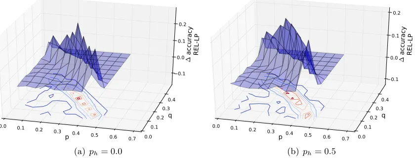
Comparison against LP. Figure 2 shows the difference in accuracy between REL and
LP as the parameters p, q, and ph change, with pif = 0.3 (the plots are almost identical
withpif= 0 andpif= 0.5). We can make the following observations:
• REL is always at least as accurate as LP, and often much more accurate. Thus,
underEdgeExplain,REL dominatesLP.
• The parameter settings for whichREL outperformsLPthe most lie almost on a line
in thepq-plane. This corresponds to p+q ≈const., which agrees with Corollary 4.
p
0.0 0.1 0.2 0.3
0.4 0.5 0.6 0.7
q
0.0 0.10.2
0.30.4
∆
accu ra cy
REL-LP
0.1 0.0 0.1 0.2
(a)ph= 0.0
p
0.0 0.1 0.2 0.3
0.4 0.5 0.6 0.7
q
0.0 0.10.2
0.30.4
∆
accu ra cy
REL-LP
0.1 0.0 0.1 0.2
(b) ph= 0.5
Figure 2: REL outperforms LP: The REL inference method under EdgeExplain
out-performsLP irrespective of the fraction of friends whose labels are hidden. The
greatest difference is whenp+q ≈const., agreeing with Corollary 4.
and label propagation is primarily a function of the relative probabilities of the various labels (thep) and the chances of various label types being used for forming friendships (theq); again, this is what we saw in Section 6.
Comparison of REL and VAR.Figure 3 compares RELagainst VAR. We observe the
following:
• Although both are algorithms for inference underEdgeExplain, they perform better
under different parameter regimes. When the labels of all friends are known perfectly (ph = 0), VARperforms better than REL. However, as ph increases, information in
the neighborhood of the ego becomes more uncertain, and REL performs better for
high ph. The transition point is around ph ≈0.1, i.e., when 90% of friend labels are
known.
• The greatest difference is in the same region of thepq-plane whereRELoutperformed LP the most.
• Withph fixed, the greatestmagnitudeof difference occurs for larger values of p.
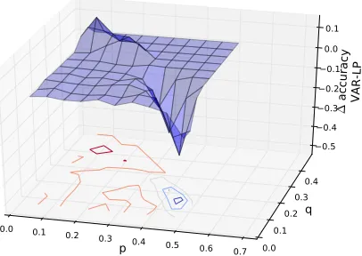
• Indeed, for large ph, VAR performs worse than even LP for large p and small q
(Figure 4).
The underlying reason is the form of the variational update (Thm. 1), in particular, in the exponentiation which serves to magnify even minor differences in its argument. When
ph is high, there are more errors in labels assigned to friends with missing information. This
leads to incorrect estimation of the chances that two nodes share a label (the parameter
p 0.0 0.1 0.2 0.3
0.4 0.5 0.6 0.7 q
0.0 0.10.2
0.30.4
∆
accu racy REL-VAR
0.2 0.1 0.0
(a)ph= 0.0
p 0.0 0.1 0.2 0.3
0.4 0.5 0.6 0.7 q
0.0 0.10.2
0.30.4
∆ ac cura cy
REL-VAR
0.2 0.1 0.0 0.1 0.2
(b) ph= 0.1
p 0.0 0.1 0.2 0.3
0.4 0.5 0.6 0.7
q
0.0 0.10.2
0.30.4
∆
accu
ra
cy
REL-VAR
0.30.2 0.1 0.0 0.10.2 0.3 0.4
(c)ph= 0.2
p 0.0 0.1 0.2 0.3
0.4 0.5 0.6 0.7
q
0.0 0.10.2
0.30.4
∆
accu racy REL-VAR
0.2 0.1 0.0 0.1 0.2 0.3 0.4
(d) ph= 0.3
Figure 3: RELversus VAR:REL is better when more friends hide their labels (ph ≥0.1).
However, when labels of all friends are known (ph = 0), VARis better.
The problem is even more acute when pis high andq is low: the lowq means that label type tis rarely shared among friends, while high pmeans that both possible labels of type
tare common (recall thatp <0.5, so a highp corresponds top≈0.5). This implies greater chances of mistakes in calculating ηuvtin the initial iterations, which is exacerbated by the
exponentiation.
However, the positive side of exponentiation is that when friend labels are not noisy (as when ph = 0), VAR converges quickly to the correct labels, while REL may get stuck in
local minima during its gradient ascent. This explains why VARis better for low ph.
7.3 A hybrid inference algorithm
The previous discussion suggests the following hybrid inference procedure: in any iteration, for any nodeu, update its label probabilities viaVAR if we are quite confident about the
labels of most of the friends ofu, otherwise use REL for the update. In effect, this tries to
useVAR andREL precisely where they worked best in the previous simulations.
Thus, HYBRID counts the fraction of friends of u whose labels are “nearly certain”
p
0.0 0.1 0.2
0.3 0.4 0.5
0.6 0.7
q
0.00.1 0.20.3
0.4
∆
accu ra cy
VAR-LP
0.5 0.4 0.3 0.2 0.1 0.0 0.1
Figure 4: VARversus LP for one parameter setting: Withph= 0.3 andpif= 0.3,VARis
better thanLP for low p, and worse for high p.
Algorithm 1 HYBRID
function HYBRID(initial label-probs,θ1,θ2) repeat
for all nodesu do
Lu = number of distinct labels inSu∼vlabel-probst(v)
nearly-certain-friends =|{v|u∼v,max(label-probst(v))>2θ1/|Lu| ∀t∈ T }| all-friends =|{v|u∼v}|
if nearly-certain-friends> θ2∗all-friendsthen Update label-probst(u) viaVAR
else
Update label-probst(u) viaREL
end if end for
until convergence or maximum iterations return label-probs(u)
end function
number of labels in the neighborhood) and applies the variational update (VAR) if this
fraction is more thanθ2, otherwise the relaxation labeling update (REL) is used.
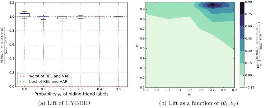
Figure 5 compares the accuracy of HYBRID to REL and VAR. Plot (a) shows, for
(θ1 = 0.7, θ2 = 0.95), the lift in accuracy of HYBRID against the others; a lift of 0
corresponds to accuracy equivalent to the worst of the two, while a lift of 1 corresponds to the best of the two. We see thatHYBRIDis in fact as good as the best of them for all ph
(recall thatVARwas better for smallph, andRELelsewhere). The results are very similar
when the probability pif of inter-friend edges is varied. Plot (b) shows a contour plot of
0.0 0.1 0.2 0.3 0.4 0.5
Probability ph of hiding friend labels
0.0 0.2 0.4 0.6 0.8 1.0 1.2 H YB R ID − m in ( R E L ,V A R ) | R E L − VA R |
worst of REL and VAR best of REL and VAR
(a) Lift of HYBRID
0.1 0.2 0.3 0.4 0.5 0.6 0.7 0.8 0.9
θ1 0.1 0.2 0.3 0.4 0.5 0.6 0.7 0.8 0.9 θ2 0.15 0.00 0.15 0.30 0.45 0.60 0.75 0.90 m
inph ³H YB R ID − m in ( R E L ,V A R ) | R E L − VA R | ´
(b) Lift as a function of (θ1, θ2)
Figure 5: HYBRID performs as well as the best of REL and VAR: (a) The lift of HY-BRID (with θ1 = 0.7 and θ2 = 0.95) over the minimum of REL and VAR is plotted againstph (restricted to parameter settings where REL and VARdiffer
in accuracy by at least 0.01); a lift of 0 corresponds to no improvement over the worst of the two, while 1 corresponds to the performance of the better of the
two. HYBRID is seen to provide better performance than REL or VAR over
the entire range of ph. (b) The minimum lift over all ph is plotted for various
(θ1, θ2) settings, with θ1 = 0.7,θ2= 0.95 performing the best.
8. Empirical evaluation
Previously, we provided intuition and examples supporting the claim that EdgeExplain
is better suited to inference of our desired label types than label propagation. In this section, we demonstrate this via empirical evidence on two large social network data sets from Facebook and Google+, and a movie network.
8.1 Evaluation on the Facebook network
We performed a study on a previously collected subgraph of the Facebook social net-work (Chakrabarti et al., 2014). 1 This data set consists of a large number of users and their friendship edges, as well as the hometown, current city, high school, college, and employer for each user, whenever these fields are available and have their visibility set to public. The dimensionality of our five label types range from almost 900K to over 6.3M. We describe below in Implementation Details our process for generating the edges. This forms our
base data set.
Evaluation Methodology. The set of users is randomly split into five parts and the
accuracy is measured via 5-fold cross-validation, with the known profile information from four folds being used to predict labels for all types for users in the fifth fold. Results over the
Hometown Current city High school College Employer
Lift of Edge−Explain o
v
er K=20
0% 20% 40% 60% 80% 100%
K
50 100 200 400
(a) Recall at 1
Hometown Current city High school College Employer
Lift of Edge−Explain o
v
er K=20
0% 20% 40% 60% 80% 100%
K
50 100 200 400
(b) Recall at 3
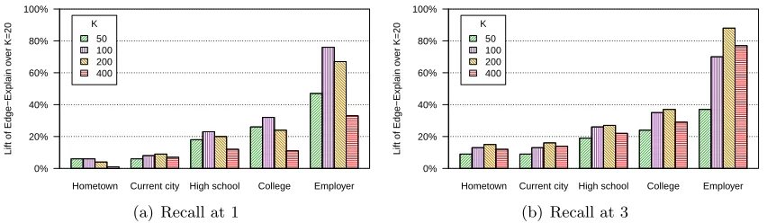
Figure 6: Recall of EdgeExplainfor graphs built with different number of friendsK: The
plot shows lift in recall with respect to a fixed baseline of EdgeExplain with K = 20. Increasing K increases recall up to a point, but then the extra friends introduce noise which hurts accuracy.
various folds are identical to three decimal places. All differences are therefore significant and we do not show variances as they are too small to be noticeable.
For each evaluation, we run inference on the training set and compute a ranking of labels for each label type for each user. This ranking is provided by the label probabilities computed by each label inference method. We then measure recall at the 1 and top-3 positions, i.e., we measure the fraction of (user, label type) pairs in the test set where the predicted top-ranked label (or any of the top-3 labels) match the actual user-provided label. For reasons of confidentiality, we only present theliftin recall values with respect to a clearly specified baseline.
Implementation Details. We implemented EdgeExplain in Giraph (Ching, 2013)
which is an iterative graph processing system based on the Bulk Synchronous Process-ing model (Malewicz et al., 2010; Valiant, 1990). The entire set of nodes is split among 200 machines, and in each iteration, every node u sends the probability distributions (fut` for REL, µut` forVAR) to all friends of u. To limit the communication overhead, we
imple-mented two features: (a) for each user u and label type t, the label distribution for each (user, type) pair was clipped to retain only the top 8 entries optimally (Kyrillidis et al., 2013), and (b) the friendship graph is sparsified so as to retain, for each useru, the topK
friends whose ages are closest to that ofu. This choice of friends is guided by the intuition that friends of similar age are most likely to share certain label types such as high school and college. We find that clipping the distributions makes little difference to accuracy while significantly improving running time. However, the value of K matters significantly, and we detail these effects next.
Accuracy of EdgeExplain. We first show how recall varies as a function of the number
of friends K. In the following, EdgeExplain with REL inference is used unless noted
otherwise; comparisons with VAR are shown later. Figure 6 shows recall versus K, with
recall at K = 20 being the baseline. We observe that recall increases up to a certain K
Hometown Current city High school College Employer
Lift of Edge−Explain o
v
er
Label Propagation
0% 50% 100%
K 20 50 100 200 400
(a) Recall at 1
Hometown Current city High school College Employer
Lift of Edge−Explain o
v
er
Label Propagation
−20% 0% 20% 40% 60% 80%
K 20 50 100 200 400
(b) Recall at 3
Figure 7: Lift of EdgeExplain over label propagation: Increasing the number of friends K benefits EdgeExplain much more than label propagation for high school,
college, and especially employer.
number of friends enables better inference but beyond a point, more friends increase noise. Thus,K ≈100 friends appear to be enough for inference underEdgeExplain.
Figure 6 also shows an increasing trend from hometown to employer in the degree of improvement obtained over the K = 20 baseline. This is because (a) the baseline itself is best for hometown and worst for employer, but also because (b) Facebook users appear to have many more friends from label types other than from their current employer. The effect of this latter observation is that if we only have a small K, it is very likely that the few friends from the same current employer are not included in that limited set of friends (which we empirically verified). As K increases and such same-employer edges become available, EdgeExplain can easily learn the reason for these edges (hence the dramatic
increase in recall), but label propagation will likely be confused by the overall distribution of different employers among all friends and therefore does not benefit equally from adding more friends, as we show next.
Comparison with Label Propagation. Figure 7 shows the lift in recall achieved by
EdgeExplainover label propagation as we increase K for both. We observe similar
per-formance of both methods for hometown and current city, but increasing improvements for high school, college, and employer. This again points to the first two label types being easier to infer, while the latter three are more difficult. With fewer employer-based friendships, the prototypical example of Figure 1 would also occur frequently, with label propagation likely picking common employers of (say) hometown friends instead of the less common friendships based on the actual employer. By attempting to explain each friendship,
Edge-Explainis able to infer the employer even under such difficult circumstances. This ability
to perform well even for under-represented label types makes EdgeExplain particularly attractive.
Effect ofα. Figure 8 shows that the lift in recall at 1 for various values of the parameter
α, with respect toα = 0.1. Performance generally improves with increasing α. Results for recall at 3 are qualitatively similar, though the effect is more muted. We find that α ∈ [10,40] offer the best results, andEdgeExplainis robust to the specific choice ofα within
Hometown Current city High school College Employer
Lift of Edge−Explain o
v
er
α
=
0.1
−10% 0% 10% 20% 30% 40% 50%
α 1 5 10 20 40
Figure 8: Effect ofα: Lift in recall at 1 is plotted for different values of α, with respect to
α= 0.1. The best results are forα∈[10,40].
Hometown Current city High school College Employer
Lift o
v
er Label Propagation
0% 20% 40% 60% 80% 100% 120% 140%
Inference VAR REL
(a) Recall at 1
Hometown Current city High school College Employer
Lift o
v
er Label Propagation
0% 10% 20% 30% 40% 50%
Inference VAR REL
(b) Recall at 3
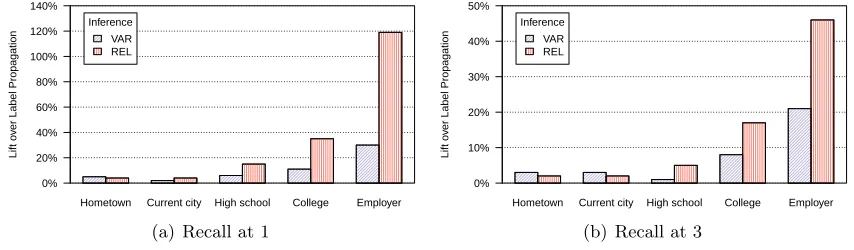
Figure 9: Comparison of VAR and REL: The lift of each inference method over label
propagation propagation is plotted for K = 100. REL is seen to outperform VAR, and both are better than LP.
while with small α, multiple matching labels may be needed. Thus, the outperformance of largeα provides empirical validation of property(P2)(on our network).
Variational inference versus Relaxation Labeling. Our two main methods for
inference under EdgeExplain are REL and VAR. Recall that while both use per-node
parameters, they attempt to optimize Eqs. 2–4 in different ways. RELrelaxes the problem
by replacing the hidden variablesSut`by their “probabilities”fut`, but the relaxed objective
is not formally related to the probabilistic model. On the other hand, VAR formally
optimizes a lower-bound on the model log-likelihood, but the lower bound may not be very tight (we note, however, that this is the standard variational assumption when per-node parameters are needed).
Figure 9 compares the two inference methods. The lift in recall of each method over LP is shown, with K = 100. While both outperform LP, REL is more accurate than VAR. This agrees with our simulation results, where VAR outperformed REL only in a
Table 1: Lift in recall from using group memberships: Inclusion of group membership barely improves recall@3, even though it is an orthogonal feature with wide coverage. Thus, information about label types is already encoded in the network structure, and careful modeling viaEdgeExplainis sufficient to extract it.
Label Type Recall at 1 Recall at 3
Hometown −0.1% 0.7%
Current city 0.4% 1.0%
High school 0.1% 0.8%
College −0.6% 1.0%
Employer −2.8% 1.2%
high confidence. Such instances are unlikely in social networks, contributing to the relative weakness of VAR.
Given the better performance of REL on this data set, the following results in this
section use REL.
Inclusion of extra features. EdgeExplaineasily generalizes to broader settings with
multiple user features, such as group memberships, topics of interest, keywords, or pages liked by the user. As an example, consider group memberships of users. Intuitively, if most members of a group come from the same college, then it is likely a college-friends group, and this can aid inference for group members whose college is unknown. This can be easily handled by creating a special node for each group, and creating “friendship” edges between the group node and its members. EdgeExplain will infer labels for the group node as
well, and will explain its “friendships” via the college label. This, in turn, will influence college inference for group members with unknown college labels. Group memberships are extensive and provide information that is orthogonal to friendships; hence, a priori, one would expect the addition of group membership features to have significant impact on label inference.
Table 1 shows the lift in recall forEdgeExplainwhen group memberships are used in
addition to K = 100 friends. While the addition of group memberships increases the size of the graph by ≈25%, the observed benefits for recall are minor: a maximum lift of only 1.2% for employer inference, and indeed reduced recall at 1 for several label types. Note that the lift in recall would have appeared very significant had we compared it to label propagation with K = 100; however, this gain largely disappears when the friendships are considered in the framework of EdgeExplain. Thus, it is not merely the scalability of
EdgeExplain, but also the careful modeling of properties (P1)-(P3) that makes group
membership redundant.
Given thea priori expectations of the impact of group memberships, this surprising re-sult suggests that information regarding our label types are already encoded in the structure of the social network and hence the orthogonal information from the group memberships actually turns out to be redundant.
The limits of resolution. Our model theoretically should be able to handle any number
0.00 0.05 0.10 0.15 0.20 0.2
0.4 0.6 0.8 1.0
Fraction of friends sharing user's true label
Probability of correct inf
erence
●
●
●
●
●
● Hometown
Current city High school College Employer
Figure 10: Probability of correctly inferring (in the top-3) the value of a given label type t
for a user, given the fraction of friends with known label fortwho actually share
the user’s label for t: All label types are broadly similar, with a fraction of 0.1
usually being sufficient for inference. For fraction>0.2, the plot flattens out.
100 200 300 400
500 1000 1500
Number of friends K
Running time (min
utes)
● ●
●
●
●
● EdgeExplain
Label Propagation
Figure 11: Running time increases linearly withK.
sharing a certain label type (say, the same college) does a user need to have in order to correctly infer the value of that label type? To answer this, we select, for each user, the set of friends whose label for the given label typetis known, and we compute the fraction that actually shared the user’s label for t. Figure 10 shows the probability thatEdgeExplain