T
T
E
E
C
C
H
H
N
N
I
I
C
C
A
A
L
L
M
M
E
E
T
T
H
H
O
O
D
D
S
S
A
A
N
N
D
D
A
A
L
L
G
G
O
O
R
R
I
I
T
T
H
H
M
M
S
S
F
F
O
O
R
R
D
D
E
E
V
V
E
E
L
L
O
O
P
P
I
I
N
N
G
G
E
E
F
F
F
F
I
I
C
C
I
I
E
E
N
N
T
T
O
O
P
P
T
T
I
I
C
C
A
A
L
L
C
C
H
H
A
A
R
R
A
A
C
C
T
T
E
E
R
R
R
R
E
E
C
C
O
O
G
G
N
N
I
I
T
T
I
I
O
O
N
N
S
S
Y
Y
S
S
T
T
E
E
M
M
:
:
A
A
N
N
O
O
V
V
E
E
R
R
V
V
I
I
E
E
W
W
Y
Ya
ak
ku
ub
bu
u
A
A.
.
I
Ib
br
ra
ah
hi
im
m
11,
,
T
Tu
un
nj
ji
i
S
S.
.
I
Ib
bi
iy
ye
em
mi
i
2 21
Department of Computer Science, Bingham University, Karu, Nasarawa State, Nigeria
2
Department of Electrical Engineering, University of Ilorin, Ilorin, Nigeria
Corresponding Author: Yakubu A. Ibrahim, [email protected] ABSTRACT: Machine recognition problem of printed
documents in Optical Character Recognition has been the target of research in the area of pattern recognition. Study in this aspect has been controlled by a need to join the natural process of image input with the data processing abilities of computer system. In this regard, engineers and scientists are not able to make judicious use of OCR systems for their technical work because they lack effective algorithms for interpretation of complex expressions even though it is important part of a Human Computer Interaction system. However, OCR in a nut shell is the electronic change of printed or handwritten text into images using machine encoding scheme representation like ASCII or Unicode. Hence, various methods and algorithms have been demonstrated in the study to increase the efficiency of system to effectively solve OCR problems. The study shows the concept of various OCR algorithms such as support vector machine, decision tree classifier, statistical, structural, artificial neural networks and template matching algorithms.
KEYWORDS: ASCII, Unicode, Computer, HCI, OCR, Pattern recognition.
I. INTRODUCTION
Pattern recognition replication of human works, like reading, is a long time vision of the researchers but in recent periods, system reading using OCR has grown to a vision established. OCR is a good application of technology progress in the area of artificial intelligence in computer vision and pattern recognition. Commercial application services exists for performing OCR for different applications, but the OCR systems are still not able to compete with human reading patterns. In this study, different technical algorithms for efficient OCR systems were critically reviewed.
II. OPTICAL CHARACTER
RECOGNITION SYSTEM
OCR system is one of the applications in pattern recognition which targets transform an image of typewritten, printed, or handwritten text into a
computer understandable form which system can easily recognize. Definitely, the OCR system is used in many applications of different domains such as: security system, mail sorting postal code recognition, bank check processing, etc. However, OCR system development is a difficult work because writing of words have an unlimited number of ways due the fact that every individual has a unique handwriting, different fonts and many styles (underlined, bold, italic, etc), with different layouts. So it all depends on the type of writing that a system should recognize operations to be performed and the results can vary significantly ([VK15]).
The handwritten or printed character recognition system can be divided into two namely: offline and online system.
a. ONLINE RECOGNITION
This is system of writing by which word recognition activity is performed efficiently at the same time the user is writing the words on the system. Printed alphabets recognition system entails the auto-transformation of written text as it is written on a unique system digitizer then a sensor follows up the tip-head of the pen for pattern prediction of the movements. The result of the signal is then transformed into codes of characters that which are usable for text-processing applications in computer ([VK15]).
b. OFFLINE RECOGNITION
recognition process is a difficult activity because different individuals and personalities have different handwriting styles and patterns ([VK15]).
III. OCR METHODS AND ALGORITHMS
The study critically reviewed the following OCR methods and algorithms ([SAA12]).
A. Statistical Algorithms
B. Template Matching Algorithm C. Neural Network Algorithms D. Structural Algorithms E. Decision Tree Classifier F. Support Vector Machine
A. STATISTICAL ALGORITHMS
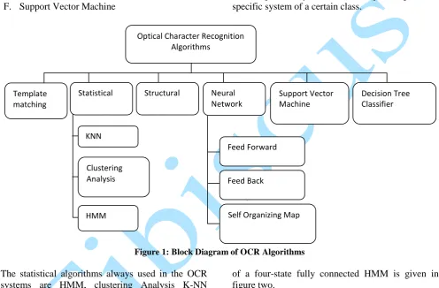
Statistical algorithms are to check for the group which the specific given pattern of recognition system belongs. During the verification and measurement process, certain set of numbers is prepared; this numbers are used to acquire a measurement vector for the pattern. The concepts from statistical decision theory are used to create decision boundaries between pattern groups. These algorithms adopt the statistical decision procedure and a set of efficiency criteria which increases in turn the probability of the observed pattern given the specific system of a certain class.
Figure 1: Block Diagram of OCR Algorithms
The statistical algorithms always used in the OCR systems are HMM, clustering Analysis K-NN ([Fuk90]).
i. HIDDEN MARKOV MODELING
HMM is basically a mathematical model in which one observes a sequence of generated emissions, but do not have the knowledge of the arrangement of states the model went through to produce the emissions. Analysis of HMMs seeks to recover the sequence of states from the observed data.
A FSM can be represented by a HMM, which however, can be represented by either a connected graph or a special pattern of connected graph called a trellis. Every given node of this graph represents a state and the signal being designed possesses a certain set of properties while each edge is a possible transition between two states at consecutive discrete time intervals. Typical example of a trellis and graph
of a four-state fully connected HMM is given in figure two.
Figure 2: (a) Trellis Diagram (b) Corresponding graph of four states HMM
Typical HMM has five distinct elements mathematically namely:
KNN
Clustering Analysis
HMM
Optical Character Recognition Algorithms
Template matching
Statistical Structural Neural Network
Support Vector Machine
Decision Tree Classifier
Feed Forward
Feed Back
i. The Internal States: The internal states are not opened and make the model to be adaptive for different system applications. A set of N states is: Q=q1,q2,…,qN
ii. The Output State: O = {o1, o2, o3, . . ., on} The output state is an observation alphabet which is a array of n observations of which each one is gotten from a vocabulary V=v1,v2,…,vn.
iii. The Transition Probability Distribution: Let A = a11, a12,…, aij be a given i by j matrix. The matrix explains the probability of transition from one state to another state. A transition probability matrix A, each aij representing the probability of moving from state i to state j,
iv. Output Observation: Probability Distribution B = {bi (k)}={P(ot=k|xt=i)} for 1≤ i ≤ N and 1≤ k ≤ K is a sequence of shown result likelihoods, also referred to as emission probabilities, each stressing the probability of an observation k being produced from a state i.
v. The initial state distribution (π = {πi} ={P(x1=i)}) where πi is the probability that the Markov chain begins in state i. some states j may have πj =0, meaning that they cannot be initial states.
Also,
. A certain initial state and final state that are not in any way related with observations, together with transition probabilities a01, a02 …a0n out of the start state and a1f, a2f, …, anf into the end state.
The probability distributions A, B and π are often shown in HMM as a compact form denoted by lambda as λ = (A, B, π) ([VK15]).
ii. CLUSTERING ANALYSIS
Clustering is the task of categorizing a set of character objects in such a way that those of the character objects in the same category are more similar to each other than to those in other categories. Clustering is used when we know that the sample units of character objects come from an unknown number of distinct population or sub-populations. It can also be assumed that the sample units of objects come from a number of distinct populations, but there is no priori explanation of those populations. The aim is to explain information of those populations using the observed data. It is generally used for exploratory data analysis and serves as a method of discovery by solving classification challenges. ([VK15]).
iii. K-NNs ALGORITHM
The k-NN adopts a non-parametric system of algorithm which can be used for character alphabet or string classification. The input character consists of the k closest training examples in the feature space. In the process of classification using this method, the result of a character is a class membership ([Fuk90]).
The k-NN model is given as follows:
(1)
Where, di is a character to be tested, xj is among the
nearest neighbors in the training set, y(xj,ck) {0, 1}
shows if xj belongs to class ck, Sim(di,xj) is the
similarity function for di. The equation (1) above
shows the class with maximal sum of similarity will be the winning class. The similarity function which is the Euclidean distance is given by the equation (2). (2) In other words, k-NN classifier requires a distance metric d, a positive integer k, and the reference templates Xm of m labeled patterns. A new input vector x is classified using the subset of k-feature vectors of that are closest x to the given distance metric d ([FH51]). Mathematically this can be described to compute the a posteriori class probabilities P(wi|x) as
(3)
where ki represents the number of vectors belonging to class wi within the subset of k vectors. The major disadvantage of this classifier is distance metric computations, which increases with the progression in number of available patterns in the reference templates ([DHS01]). Pattern x is assigned to the class wi with the highest a posteriori class probability P(wi|x).
A. TEMPLATE MATCHING ALGORITHM
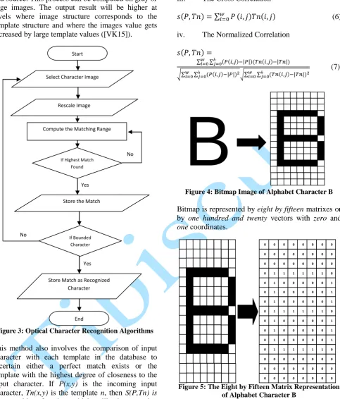
and source. This process can be computed on gray or edge images. The output result will be higher at levels where image structure corresponds to the template structure and where the images value gets increased by large template values ([VK15]).
Figure 3: Optical Character Recognition Algorithms
This method also involves the comparison of input character with each template in the database to ascertain either a perfect match exists or the template with the highest degree of closeness to the input character. If P(x,y) is the incoming input character, Tn(x,y) is the template n, then S(P,Tn) is the matching function which will give a value showing how perfect template n matches the incoming input character. Some existing matching functions formulas are listed as follows:
i. The city block
(4)
ii. The Euclidean distance
(5)
iii. The Cross Correlation
(6) iv. The Normalized Correlation
(7)
Figure 4: Bitmap Image of Alphabet Character B
Bitmap is represented by eight by fifteen matrixes or by one hundred and twenty vectors with zero and one coordinates.
Figure 5: The Eight by Fifteen Matrix Representation of Alphabet Character B
Perfect recognition is obtained by identifying which Tn generates the perfect value of pattern matching functions, S(P,Tn). The technique can be efficient if the incoming character and templates are of the similar font ([VK15]).
The template matching technique can be performed with the following steps:
i. The character from the known string is selected. ii. The character to the font of the first template is resized.
ii. The pattern matching metric is executed.
No
Yes Yes
No Start
Select Character Image
Rescale Image
Store Match as Recognized Character
End
If Bounded Character
Compute the Matching Range
Store the Match
If Highest Match
Found
B
iv. The perfect match observed is saved. If the character did not match repeat the stage three again. v. The index of the perfect match is saved as the recognized character.
The image is converted into eight by fifteen bitmap. Template matching systems were developed as a result to the issue of object recognition, and they contain at least completely the idea of identity comparison. The representations conceived by template systems contain much more detailed information about stimulus structure than do the element representations just explained. These systems are normally applied to spatially extend visual objects, and their representation can be spatially arranged. The basic idea of this algorithm is the reference points. Reference points are points at the center of space regions in 3-Dimension spatial form. For this particular system, the regions were defined as an x, y, z center point, and three distance values, one for each axis. Alternately, by increasing and decreasing the distance values along the correct axis about the center point, a region in cube shape is formed. A possible way would be to define a radius, a point, and a sphere as the region. The source of the coordinate system is given to be the center of the subject's right shoulder socket. Since the data from the wrist tracking sensors is normalized to this origin, it is relatively easy to determine which reference point region the sensor is in at any given point in time. However, reference point regions are given to correspond to the areas of the sensors when gestures are performed. When negating the left/right axis value for the center point, a symmetric set of regions is given for the right hand sensor.
B. NEURAL NETWORK ALGORITHM
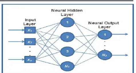
This model is a way of processing information through the use of human biological nervous systems such as the brain. It is consists of many interconnected processing elements working in together to solve certain issues ([Bis95]). The basic layers are input-hidden-output, the input layer, however, is used to feed all the input data into the network, which is followed by a hidden layer of neurons for further processing of data and the output layer for calculates the desired result of the neural network produced ([Bis95]).
i. Input Layer
The input stage is the level through which the external world sends a pattern to the network and encodes it into a sweet able form for the system. Every given input has some independent variable that has a control over the output of the neural network ([Fio01]).
Figure 6: Typical ANN Architecture
The number neurons present at the input in OCR is the number of chunks called pixels that might represent any given character. A character which represents 8 by 15 grids has shown in figure five has about one hundred and twenty pixels. Therefore, it has one hundred and twenty input neurons.
ii. Hidden Layer
The hidden layer is the level of the network which cannot directly communicate with the external world. To know the actual number of neurons in this layers is as crucial as determining the overall structure of the neural network. Various rule-of-thumb techniques are available for determining the exact number of neurons to in the hidden layers, such techniques includes:
i. Hidden neurons’ number should fall between the number size of the input level and the number size of the output level. ii. Hidden layer neurons’ should be two-third
in number the size of the input level, plus the size of the output level.
iii. The number of hidden neurons should be less than twice the size of the input level. iii. Output Layer
This layer of the network presents a pattern to the external world. However, the produced number of output neurons should be directly equal to the type of task performed by the network. The number of output layer used by the OCR system varies depending on the number of alphabet characters the system has been trained to recognize. In the same vein, presenting a specific pattern to the input neurons triggers the appropriate output neuron that corresponds to the letter that the input pattern represents ([SSP03]).
In a network, each node performs some simple calculations, and each connection transmits a signal from one node to another, labeled by a number called the connection strength showing the extent to which a signal is extended.
C. SYNTACTIC/STRUCTURAL ALGORITHM
The repetitive description of a large pattern in terms of simpler patterns based on the shape of the character was the initial knowledge behind the creation of structural recognition system. The method classifies the input patterns on the basis of parts of the characters and the relationship among these parts. At the initial stage, the prehistory of a given character is available and known therefore strings of the prehistory are observed on the basis of pre-assumed rules. Pattern syntactic model is predictably encouraging because apart from the group classification, the method also gives description on how the given path can be produced from the prehistory. Generally speaking, a given object is represented as a production rules structure, whose left-hand-side represents the character labels and whose right-hand-side represents the string of prehistory. The right-hand-side of production rules is compared to the string of prehistory extracted from a word. So classifying an object like alphabet characters means finding a path to a terminal node of the tree ([HK01]).
D. DECISION TREE
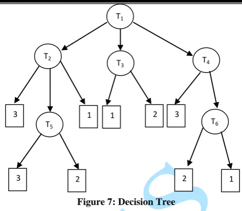
A decision tree is a technique that has multilevel decision making process which instead of using the whole features completely to make a choice; different subsets of features are used at different stages of the tree. The decision tree classifier is breaking down of complex problem into smaller, more solvable whereby it represents the relationship among attribute and decision in a tree-like diagram. The classification is generated by algorithm that shows many ways of dividing a data into branch-like tree component. The compartments normally consists three structures; the root node that has no incoming edges and zero or more outgoing edges, internal nodes that have exactly one incoming edge and two or more outgoing edges and the leaf nodes that have exactly one incoming edge and no outgoing edges. Generally, tree induction and pruning are two basic processes in Decision tree classifier system. Tree induction is an iterative training process that enables splitting of attributes into smaller subsets. The training process starts by checking the complete dataset to find the condition attributes which when selected as a splitting rule, will result in nodes that are most different from each other particularly to the expected class. Thereafter, the tree will be generalized in pruning process by removing least reliable tree branches and accuracy will be improved ([RK13]).
Figure 7: Decision Tree
The structure of a decision tree classifier can be decomposed into following tasks:
A Decision tree is a tree in which each branch node stands a choice between a numbers of alternatives, and each leaf node represents a decision ([RK13]). In the decision tree, internal nodes and the root contain attribute test conditions to separate records that have different characteristics.
i. The proper choice of tree structure.
ii. The decision of feature subsets are adopted at every internal node.
iii. The decision of the rule to be adopted at each internal node.
E. SUPPORT VECTOR MACHINE
SVM is machine learning algorithms adopted to execute classification related problems. SVM is most recent model in comparison to other supervised classification methods; it is as a matter of fact mainly based on statistical learning theory. SVM is a classification algorithm method ([BGV92]). The SVM classifier is well known method adopted in bioinformatics and other disciplines because of it has high accuracy, capability to handle high-dimensional data (e.g. gene expression), and flexibility in modeling data from many sources. SVM classification method belongs to the many categories of kernel methods. A kernel method is an algorithm is dot-products that depend on the given data. However, the dot product in this regard can be changed by a kernel function which calculates a dot product in possibly high dimensional feature vector. The advantages are the efficiency to produce non-linear decision boundaries when methods designed for linear classifiers are used and the kernel functions enables us to apply a classifier to data that have no vivid fixed-dimensional feature vector space representation ([SC04]). SVM modeling was initially used to optimize the linear hyper plane
3
T1
1 T3
T5
T2 T 4
1 2 3 3 2
T6
which separate two classed. That is, the empty region around the decision boundary determined by the distance to the nearest training pattern ([Vap95]). The basic idea behind any SVM is to map the given input data onto a higher dimensional feature space nonlinearly associated to the input space and determine a dividing hyper plane with optimum margin between the feature space of the two classes. The system, however, ensures that the higher the margin the lower is the generalization error of the classifier.
In figure 8, L1 does not divide the two classes of objects; L2 divides the two classes but with a very small margin between the classes of objects while L3 on the other hand, divide the two classes of objects with much better and clearer margin than L2. If such hyper plane exists, it is vividly clear that it gives the best separation border between the two classes and it is known as the maximum-margin hyper plane. Such a linear classifier is referred to as the maximum margin classifier.
Figure 8: Separation hyper planes
A SVM is a maximal margin hyper plane in feature space built by using a kernel function in gene space. This results in a nonlinear boundary in the input space. The optimal separating hyper plane can be achieved without any computations in the higher dimensional feature space by using kernel functions in the input space ([DHS01]). Kernel functions are class of methods for pattern analysis whose best known member is SVM. The task of pattern analysis is to find and study general types of relations (for example, classifications, correlations, clusters, etc) in datasets. The commonly used kernels include:- i. Linear Kernel:
(8) ii. Radial Basis Function (Gaussian) Kernel:
(9) iii. Polynomial Kernel:
(10)
For multiple classification, binary SVMs are combined in either one or one-against-all (pair wise) scheme. The RBF kernel on two samples x and y represented as feature vectors in some input spaces is defined in equation (9). Where δ is the free parameter. Since the value of RBF kernel decreases with distance and ranges between zero and one, it has a ready interpretation as a similarity measure ([Bis95]).
a. One Against All
One against all strategy consists of generating one SVM one class to divide its members from members of other classes.
Ideally, group classification of an unknown pattern is performed according to the maximum result output among all SVMs ([DKS03]).
Figure 9: One against all region boundaries on a basic problem
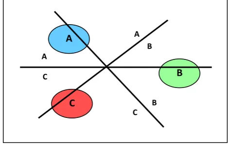
b. One Against One
One against one is one of the foremost methods of simplifying the decisions made within multilevel classification.
Figure 10: One against one region boundaries on a basic problem
It is thought to maximize performance among multilevel classification methods by reducing a multilevel problem to binary ones, as it is simpler to make predictions for two sets than ones with multiple classes.
B A
C
A
C
C B A
B
B A
C
L1
L3
Normally, group classification of an unknown given pattern is performed according to the maximum voting, where each SVM casts for one class.
IV. CONCLUSION
The optical character recognition is an active research area, but more efforts concern the efficient algorithms to be used for recognition need to be put in place. In the study, a large number of OCR algorithm methods for implementing efficient OCR system were shown. Hence, the issue of method or algorithm selection for efficient optical character recognition as to maximize performance of the OCR system when given a hard time limit within which we need to provide a solution is solved.
REFERENCES
[Bis95] C. M. Bishop - Neural Networks for Pattern Recognition, Calderon Press, Oxford, 1995.
[BGV92] B. E. Boser, I. M. Guyon, V. N. Vapnik - A training algorithm for optimal margin classifiers. In D. Haussler, editor, 5th Annual ACM Workshop on COLT, pages 144-152, Pittsburgh, PA, 1992. ACM Press. [DHS01] R. O. Duda, P. E. Hart, D. G. Stork -
Pattern Classification, Wiley, New York, 2nd edition edition, 2001.
[DKS03] J. X. Dong, A. Krzyzak, C. Y. Suen - High accuracy handwritten Chinese character recognition using support vector machine, Proc. Int. Workshop on Artificial Neural Networks for Pattern Recognition, Florence, Italy, 2003. [Fio01] N. Fiona - Neural Networks –
algorithms and applications, 2001.
[Fuk90] K. Fukunaga - Introduction to Statistical Pattern Recognition, 2nd edition, Academic Press, 1990.
[FH51] E. Fix, J. L. Hodges - Discriminatory
analysis - nonparametric
discrimination: Consistency properties, Tech. Rep. Project 21-49-004, Report No.4, USAF School of Aviation Medicine, Randolph Field, TX, 1951. [HK01] J. Han, M. Kamber - Data mining
concept and technique, San Francisco: Morgan Kaufmann Publishers 2001. [RK13] L. Rajendra, S. M. Kharad - Review
of Classification Methods for Character
Recognition in Neural Network,
International Journal of Electronics Communications and Computer Engineering, Vol. 4, Issue 2, 2013. [SC04] J. Shawe-Taylor, N. Cristianini -
Kernel Methods for Pattern Analysis. Cambridge UP, Cambridge, UK, 2004. [SAA12] G. D. Suruchi, C. A. Anjali, S. M.
Ashok - Survey of Methods for Character recognition, International Journal of Engineering and Innovative Technology (IJEIT),Volume 1, Issue 5, May 2012.
[SSP03] P. Y. Simard, D. Steinkraus, J. C. Platt - Best practices for convolutional neural networks applied to visual document analysis, Proc. 7th ICDAR, Edinburgh, UK, 2003, Vol.2, pp.958-962.
[Vap95] V. Vapnik - The nature of statistical Learning Theory. Springer, N.Y. ISBN 0-387-94559-8, 1995.