Journal of Hydraulic Structures J. Hydraul. Struct., 2019; 5(1):42-59
DOI: 10.22055/jhs.2019.29625.1113
Forecasting of rainfall using different input selection methods
on climate signals for neural network inputs
Alireza B Dariane 1
Mohammadreza Ashrafi Gol2
Farzaneh Karami 3
Abstract
Long-term prediction of precipitation in planning and managing water resources, especially in arid and semi-arid countries such as Iran, has great importance. In this paper, a method for predicting long-term precipitation using weather signals and artificial neural networks is presented. For this purpose, climate data (large-scale signals) and meteorological data (local precipitation and temperature) with 3 to 12 months lead-times are used as inputs to predict precipitation for 3, 6, 9 and 12 months periods in 6 selected stations across Iran. A genetic algorithm (GA) and self-organized neural network (SOM) along with the application of winGamma software were comparatively used as input selection methods to choose the appropriate input variables. Examining the results, out of 96 predictions performed at all stations, in 43 cases, GA, in 28 cases, winGamma, and in 25 cases SOM have the best results compared to the other two methods. According to this, as a generalized assumption, it can be said that at least for the selected stations in this paper, the GA method is more reliable than the other two methods, and can be used to make predictions for future applications as a reliable input selection method. Moreover, among different climatic signals, Pacific Decadal Oscillation (PDO), Trans-Niño Index (TNI) and Eastern Tropical Pacific SST (NINO3) are the most repetitive indices for the most accurate forecast of each station.
Keywords: Precipitation Prediction, Large Scale Climatic Signals, Self-Organized Artificial Neural Networks, Input Selection Method, Genetic Algorithm.
Received: 19 May 2019; Accepted: 21 June 2019
1 Water Resources Division, Department of Civil Engineering, KN Toosi University of Technology, Tehran, Iran, [email protected] (Corresponding author).
2 Department of Civil Engineering, KN Toosi University of Technology, Tehran, Iran,
3 Department of Civil Engineering, KN Toosi University of Technology, Tehran, Iran,
1. Introduction
Iran is located in a region with diverse climatic conditions. This means that it includes the arid climate beside temperate and mountain climates. Due to the particular situation of Iran, which is connected to high seas on the one hand and dry lands on the other hand, several factors affect the climate including winds, climate signals and other monsoonal and seasonal phenomena.
Nowadays, the application of climatic signals and climatological data has been considered for prediction of streamflow, precipitation or temperature in a region. Researchers have tended to use large-scale climatic signals in water resources management in recent years for the following reasons:
1. Increase in awareness and information about large-scale climate data and their relationship with hydrologic and meteorological variables
2. Climate change and its impacts on water resources
3. The occurrence of floods and droughts with higher intensities in many parts of the world in recent years
In addition to the above reasons, studies have shown that the use of large-scale climatic signals can enhance the accuracy of predictions and increase the time interval (up to several months). Moreover, hydrologic analyzes can be increased and be more accurate by taking into account the climate statistics.
coastal areas of the Caspian Sea decreases from east to west, and its impact on the northern part of the Alborz is lower than the southern slops [6].
Curtis et al. (2001) examined the relation between the changes in rainfall in the Mediterranean parts of Europe and ENSO. The results obtained by them indicate the significant impact of ENSO on the Mediterranean rainfall in Europe. They showed that, although the absolute value of rainfall variation is lower than that of normal in these areas compared to the tropics, these changes, especially in the Mediterranean region, are directly related to the phenomenon of ENSO [7]. Cullen et al. (2002) examined the relation between the NAO and the rainfall and streamflow of major rivers in the Middle East such as Sobhon, Tigris, Euphrates, Karun, Yarmouk and Jordan. For this purpose, two seasons were considered for analyzing the streamflow changes of these rivers. The results of this study showed that the streamflow from December to March is affected by the NAO phenomenon. Results have shown that the effect of NAO on rainfall and temperature in the Middle East is lower during April-June, and the streamflow in this period is more affected by snow and snow melting parameters [8]. As new techniques were developed, they were employed to explore better relations between the long-range climatic signals and the local climatic data. Pineda and Willems (2018) presented a statistical analysis framework to mine climate data and separate weather and climate controls using data-driven process identification. The model investigated the climatological forcing hypothesis leading to anomalous rainfall extremes [9]. Kisembe et al. (2018) investigated the ability of the models to capture the influence of large-scale features such as ENSO on Ugandan rainfall [10]. Armal et al. (2018) presented a systematic analysis for identifying and attributing trends in the annual frequency of extreme rainfall events across the contiguous United States to climate change and climate variability modes [11].
Jeong and Kim (2004) used the ESP technique to obtain a one-month-long streamflow forecast for the Chungju Reservoir in the Han River Basin [12]. Kumar et al. (2007) used neural networks for monthly and seasonal predictions (from June to September) based on large scale satellite signals in Orissa, eastern India. They used genetic algorithms to train the neural network architecture. One of the most prominent points of this research was that seasonally predicted outcomes were better than monthly estimates. The researchers believe that the main reason for this is the variability in the nature of climate variables, which creates more uncertainty on a monthly basis than season [13]. Salas et al. (2011) used atmospheric, oceanic and hydrologic indicators for long term forecasting of the Colorado River flow with seasonal and annual time steps [14]. Zahraie et al. (2004) presented a method for prediction of high and low rainfall in the Karun basin [15].
non-heavy rain weather by using weather data [20]. Venkadesha et al. (2013) developed ANN models to predict air temperature by performing a GA input selection method [21]. Dariane and Azimi (2016) used a combination of GA input selection method and Neuro Fuzzy Inference System for Forecasting streamflow [22]. Remesan et al. (2008) demonstrated the informative capability of the Gamma test in the selection of relevant variables in the construction of nonlinear models [23]. Rauf et al. (2016) presented a method as a foundation of early warning for the reduction and mitigation of flood disasters, and decision making for scientific flood dispatching. They performed Gamma tests in WinGamma and made nonlinear models of 500 different combination [24]. Singh et al. (2018) used WinGamma to select the best combination of input variables for daily rainfall-runoff modeling with neuro-fuzzy inference system and multi-layer perceptron neural network [25].
The purpose of this study is to predict precipitation using artificial neural network and exploiting large scale climatic signals as well as precipitation and temperature of past years for selected stations. For this purpose, first, the weather data (temperature and precipitation) and climate signals should be extracted for a long period of time and then, according to different methods, the appropriate prediction method should be selected. Since the frequency of data is very high and variables are diverse, three input selection methods including GA, winGamma software and also SOM were used to select variables. Initially, different variables and parameters are selected for different regions and a set of them are entered as input parameters into the model, then the model is compiled and implemented. In order to reach more accurate results, several neural networks with different input data are created and by averaging them the rainfall and temperature are predicted for different time horizons (3, 6, 9 and 12 months).
.
2. Case Study
Figure 1. Locations of different stations scattered throughout the country
Table 1. Average annual precipitation and temperature for the selected stations
Station Height (m)
Average annual precipitation
(mm)
Average annual temperature (°C)
1 Bandar Abbas 9.8 185 22
2 Mashhad 999.2 238 16
3 Iranshahr 1370 92 20
4 Urmia 1328 341 12
5 Mehrabad 1191 428 18
3. Methodology
3.1. Dataset
The study employs climate data obtained from different institutes presented in Table 2. Climatic indicators from1 to 23 in Table 2 refer to the oceans. The list of these indicators is available on the NASA National Weather Climate Center's website [26]. As these indicators relate to a particular region, research studies have shown that the correlation between these indicators in each basin area may not lead to a required result and subsequently, they will not be considered as strong predictors. For example, the NINO3 index refers to a region with a S5-N5 and W150-W90 geographic location [27]. Indicators 24-29 are related to NCEP where the time series are produced by specifying the appropriate latitude and longitude coordinates with the target area (with a precision of 2.5 °) [28]. The list of time series of these indicators is also available online. Researches have shown that these types of indicators can establish a higher correlation in comparison with indices such as PDO, SOI or NINO3 [27]. The Omega index indicates the wind velocity at different atmospheric pressures.
The variables are selected with three methods of input selection such as genetic algorithm, winGamma software and self-organized neural network. Dealing with data driven models, it is common to divide the data sets into two parts of the training and testing. The training data set are applied to tune the model parameters while the latter one is employed to evaluated performance of the developed model. A 30-year period data from 1979 to 2014 was used for training the models while a 6-year data remained for testing purpose.
3.2.Methods
As stated, the main purpose of this research is to predict rainfall using large-scale climatic signals and artificial neural network utilization. To determine the most important signals for rainfall in the stations, GA, winGamma and SOM methods have been used. Details are discussed in the following sections. Then, the effective signals are arranged in order of importance. After finding the effect of each signal, the most effective ones are selected to feed artificial neural network as input variables in order to forecast the rainfall over the study area. The artificial neural network models were developed and implemented in MATLAB. The MATLAB package has the ability to design, learn and evaluate the artificial neural network and also includes different networks with different learning rules. Dealing with neural networks, different algorithms and structure can be applied for learning process of the model However, in hydrological studies, the use of leading networks and backpropagation methods have been most widely used due to their easily implementation, simplicity and suitable performance [29].
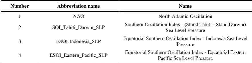
Table 2. List of climatic models used for simulation
Number Abbreviation name Name
1 NAO North Atlantic Oscillation
2 SOI_Tahiti_Darwin_SLP Southern Oscillation Index - (Stand Tahiti - Stand Darwin) Sea Level Pressure
3 ESOI-Indonesia_SLP Equatorial Southern Oscillation Index - Indonesia Sea Level Pressure
5 AMO Atlantic Multidecadal Oscillation (unsmoothed)
6 AMM Atlantic Meridional Mode
7 PNA Pacific North American Index
8 TNA Tropical Northern Atlantic Index
9 NINO3 Eastern Tropical Pacific SST
10 MEI Multivariate ENSO Index
11 PDO Pacific Decadal Oscillation
12 AO Arctic Oscillation
13 NINO1+2 Extreme Eastern Tropical Pacific SST
14 NINO3.4 East Central Tropical Pacific SST
15 NINO4 Central Tropical Pacific SST
16 EA East Atlantic index
17 EAWR Eastern Asia/Western Russia
18 SCAND Scandinavia
19 PE Polar/Eurasia Index
20 WP West Pacific Index
21 ONI Oceanic Nino index
22 BEST Bivariate ENSO Time series
23 TNI Trans-Niño Index
24 GH600 NCEP 600 mb Geopotential Height
25 AT700 NCEP 700 mb Air Temperature
26 RH600 NCEP 600 mb Relative Humidity
27 SP NCEP Surface Pressure
28 SPR NCEP Surface Precipitation Rate
29 O600 NCEP 600 mb Omega
3.2.1. Neural network
performance in any iteration. Through a repetitive process, the weights are adjusted until to meet the model stopping criteria or to reach a determined number of iterations. Generally, a usual neural network can be mathematically expressed as follows:
2 1
1 1
M N
k kj ji i jo ko
j i
O g w g w x w w
= =
= + +
(1)Where xi = the input value to node i , Ok = the output at node k , g1 = activation
function for the hidden layer and g2= activation function (linear) for the output layer. N
and M represent the number of neurons in the input and hidden layers, respectively. w jo
and wko are biases of the jth neuron in the hidden layer and the kth neuron in the output
layer. w ji is the weight between the input node i and the hidden node j , and wkj the
weight between the hidden node j and the output node k . The appropriate values for weights and biases are obtained through training process.
In the neural network, the data are divided into three parts: training, validation and testing. Validation data is used to prevent over-training. Backpropagation method is commonly used to train the neural networks. Dealing with neural networks, there are a number of parameters that should be properly tuned to achieve reliable forecasts. Number of neurons, iterations and effective variables are among the common factors require special care to construct an appropriate model. In this study, a sensitivity analysis was conducted to find the optimum number of neurons in the hidden layer. Moreover, the Nash-Sutcliff (Nash) coefficient was employed to evaluated performance of the predictive models.
3.2.2. Binary Genetic Algorithm (GA) as Input Selection Method
the greatest impact, but are not in conflict with other parameters of selection and do not have a negative effect on the whole model.
For more explanation, suppose that there are n variables which each of them may be related to the objective function with a coefficient. The binary method is used to select the appropriate variables, meaning that each chromosome consists of n single-bit genes of zero and one. Choosing a zero number in each gene means not choosing that variable as an effective input variable in the model, and vice versa, if the gene value is 1, the corresponding variable is chosen. At first a random population of chromosomes is created. Then, the variables selected on each chromosome are considered as inputs of the neural network model. The neural network is then trained by backpropagation method. In the next step, using the trained network, the results of the model are estimated for the test set and the Nash-Sutcliff index is calculated. In this step, the new generation of chromosome populations is based on the Nash index and the selection, combination and mutation operators. This process is repeated as long as no appreciable change is made in the Nash's objective function from generation to generation.
3.2.3. winGamma Software
Th winGamma software based on gamma test is a suitable proxy for nonlinear modeling. Gamma test is essentially a nonlinear modeling that investigates the relationship between input and output in a set of data. Therefore, using this software, it is easy to examine the relationship between the input parameters considered in this study with the desired output and determine the best combination of inputs. For this purpose, the results of the genetic algorithm are investigated and the combination with lower standard error and gamma content is selected as the appropriate input composition. Also, in using M-Test, the software creates a gamma graph after data scrutiny [31]. Concerning gamma test, small values of gamma demonstrate strong predictive relationship between input and target variables. On the other hand, large values of gamma denote there is no significant relationship between the input and output values. Unlike traditional linear regression measuring goodness of fit to a line, the gamma test explores goodness of fit to all smooth curves.
3.2.4. Self-Organized Map Neural Network (SOM)
may increase complexity and computational time of many data driven models. A SOM network has two modes of training and mapping in which the training mode uses input examples to build the map and subsequently the aping process is employed to classify the new input data. To build the map, training or learning process is needed to derive a pattern based on input variables. This is partially similar to structure of human brains. To construct a reliable model, a large number of example vectors as close as possible the kinds of vectors expected during mapping should be used to feed the network. In the training stage, competitive learning procedure is employed where the neurons compete for the right to respond to a subset of the input data. Assume a training example is fed to the network, the Euclidean distance of the sample to all weight vectors is computed to find the neuron with the most similar weight vector called the best matching unit. The weight of best matching unit and the neurons in its neighborhood is modified based on the input vector. However, neurons with farther distance expect to experience smaller changes. This process is repeated for any other input fed to train the SOM network. In brief, the weight of a neuron v with weight vector Wv(s) is updated as follows:
(
1)
( ) (
, ,)
.(
( )
( )
)
v v v
W s + =W s +
u v s D t −W s (2)where s is the step index,
(
u v s, ,)
is the neighborhood function denoting distance between neuron v and the neuron of best matching unit in step s ,
( )
s is a decreasing coefficient, and D t( )
represents the input vector. It is readily acknowledged that the study is not going to delve into basic concepts of the method. For more details one can refer to [32]. In this research, MATLAB software has been used to implement this method.4. Results
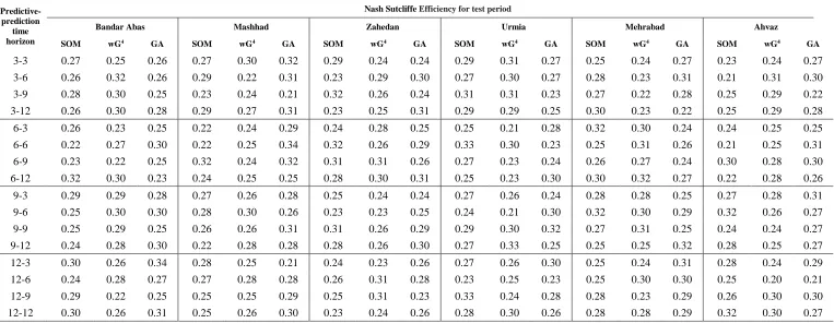
In this section the results are presented for different stations.observed precipitation and temperature and climate signals were used for precipitation forecasting with time horizons of 3, 6, 9 and 12 months. The results obtained from the three methods of input selection, GA, winGamma software and SOM, for neural network inputs are presented in Table 3. In this table, for example, 3-6 indicates the use of 3-month average data as predictor for forecasting the 6-month time horizon.
Table 3. Results of different models for selected stations
Predictive- prediction
time horizon
Nash Sutcliffe Efficiency for test period
Bandar Abas Mashhad Zahedan Urmia Mehrabad Ahvaz
SOM wG4 GA SOM wG4 GA SOM wG4 GA SOM wG4 GA SOM wG4 GA SOM wG4 GA
3-3 0.27 0.25 0.26 0.27 0.30 0.32 0.29 0.24 0.24 0.29 0.31 0.27 0.25 0.24 0.27 0.23 0.24 0.27
3-6 0.26 0.32 0.26 0.29 0.22 0.31 0.23 0.29 0.30 0.27 0.30 0.27 0.28 0.23 0.31 0.21 0.31 0.30
3-9 0.28 0.30 0.25 0.23 0.24 0.21 0.32 0.26 0.24 0.31 0.31 0.23 0.27 0.22 0.28 0.25 0.29 0.22
3-12 0.26 0.30 0.28 0.29 0.27 0.31 0.23 0.25 0.31 0.29 0.29 0.25 0.30 0.23 0.22 0.25 0.29 0.28
6-3 0.26 0.23 0.25 0.22 0.24 0.29 0.24 0.28 0.25 0.25 0.21 0.28 0.32 0.30 0.24 0.24 0.25 0.25
6-6 0.22 0.27 0.30 0.22 0.25 0.34 0.32 0.26 0.29 0.33 0.30 0.23 0.25 0.31 0.26 0.21 0.25 0.31
6-9 0.23 0.22 0.25 0.32 0.24 0.32 0.31 0.31 0.26 0.27 0.23 0.24 0.26 0.27 0.24 0.30 0.28 0.30
6-12 0.32 0.30 0.23 0.24 0.25 0.25 0.28 0.30 0.31 0.25 0.23 0.30 0.30 0.32 0.27 0.22 0.28 0.26
9-3 0.29 0.29 0.28 0.27 0.26 0.28 0.25 0.24 0.24 0.27 0.26 0.24 0.28 0.28 0.25 0.27 0.28 0.31
9-6 0.25 0.30 0.30 0.28 0.30 0.26 0.23 0.23 0.25 0.24 0.21 0.30 0.32 0.30 0.29 0.32 0.26 0.27
9-9 0.25 0.29 0.25 0.26 0.26 0.31 0.31 0.26 0.29 0.29 0.30 0.32 0.27 0.31 0.25 0.24 0.24 0.27
9-12 0.24 0.28 0.30 0.22 0.28 0.28 0.28 0.26 0.30 0.27 0.33 0.25 0.25 0.25 0.32 0.28 0.25 0.27
12-3 0.30 0.26 0.34 0.28 0.25 0.21 0.24 0.23 0.26 0.27 0.26 0.30 0.25 0.24 0.31 0.28 0.24 0.29
12-6 0.24 0.28 0.27 0.27 0.28 0.28 0.26 0.31 0.28 0.23 0.25 0.23 0.25 0.30 0.30 0.25 0.20 0.21
12-9 0.29 0.22 0.25 0.25 0.25 0.29 0.25 0.31 0.23 0.33 0.24 0.28 0.28 0.23 0.29 0.26 0.30 0.30
12-12 0.30 0.26 0.31 0.25 0.26 0.30 0.23 0.24 0.26 0.28 0.30 0.26 0.28 0.28 0.29 0.32 0.30 0.27
At Mashad station, the best prediction for the 3-month horizon is obtained from the average 3-month data (3-3) and GA method, with Nash of 0.32. For the time horizons of 6, 9 and 12 months, the most accurate predictions are for the mean of 6 (6-6), 6 (6-9) and 3 months (3-12), and the GA, SOM and GA methods, with Nash of 0.37, 0.32, and 0.31, respectively. GA provides the best forecast for 11 cases and this indicates the absolute superiority of GA at this station. Moreover, TNA, NINO3, MEI, PDO, EAWR, O600, RH600 and SP are the selected climate indices for the most accurate forecast (6-6) in Mashhad station.
At Zahedan station, the best prediction for the 3-month horizon is obtained from the mean 3-month (3-3) and SOM method, with Nash of 0.29 for the test period. For the time horizons of 6, 9 and 12 months, the most accurate predictions are for the mean of 6 (6-6), 3 (3-9) and 6 months (6-12), and GA, SOM and GA. The Nash indices are 0.32, 0.32, and 0.31, for the test period respectively. For 16 predictive states, GA provides the most accurate results with 7 times and this is 3 and 6 times for winGamma and SOM. Of the 16 different modes in this station, in 7 modes of the GA method, 3 modes of the winGamma mode and 6 modes, the SOM method has the most accurate predictions, which indicates the relative superiority of the GA method. Moreover, NAO, AO, NINO3.4 and RH600 are the selected climate indices for the most accurate forecast (6-6) in Zahedan station.
Results for Urmia, Mehrabad and Ahwaz stations are illustrated in Figure 3. At Urmia station, the best result for the 3-month time horizon is obtained from the average 3-month data and the winGamma method, with a Nash index of 0.31. In addition, for the periods of 6, 9 and 12 months, the highest accuracy are obtained from the mean of 6, 12, and 9 months data by SOM, SOM and winGamma, respectively, in which the amount of Nash indices are 0.33, 0.34 and 0.33. In this station, winGamma with 7 times superiority has better performance in comparison with GA and SOM with 5 and 4 times superiority. Moreover, PNA, PDO, NINO3 and TNI are the selected climate indices for the most accurate forecast (12-9) in Urmia station.
At Mehrabad station, the most accurate predictions for time horizons of 3, 6, 9, and 12 months were SOM, SOM, winGamma and GA, using the mean of data 6, 9 , 9 and 9 months. The values of the Nash index in each of these forecasts are 0.32, 0.32, 0.31 and 0.32, respectively. Of all the predicted states, GA, winGamma and SOM obtain the best results 7, 5 and 4 times. Therefore, at the Mehrabad station, the GA method has more acceptable accuracy than the other two methods. Moreover, NAO, Stand Tahiti-Stand Darwin, SOI_Tahiti_Darwin_SLP, AMO, NINO4, PE, TNI and SP are the selected climate indices for the most accurate forecast (9-12) in Mehrabad station.
Figure 4. Circle diagram for the contribution of each signal
Examining the results, out of 96 predictions performed at all stations, in 43 cases, GA, in 28 cases, winGamma, and in 25 cases SOM have the best results compared to the other two methods. According to this, as a generalized assumption, it can be stated that at least for the selected stations in this paper, the GA method is more reliable than the other two methods, and can be used to make predictions for future applications as a reliable input selection method. Moreover, among different climatic signals, PDO, TNI and NINO3 are the most repetitive indices for the most accurate forecast of each station. Figure 4 shows the circle diagram for the contribution of each signal.
5. Conclusion
The purpose of this study was to predict rainfall using artificial neural network and utilizing large scale climatic signals as well as observed rainfall and temperature of past years. For this purpose, at 6 stations in Iran (including Bandar Abbas stations in Hormozgan province, Mashhad in Khorasan Razavi province, Zahedan in Sistan and Baluchestan province, Urmia in West Azarbaijan province, Mehrabad in Tehran province, and finally Ahvaz in Khuzestan province) with different weather conditions were selected. Due to the abundance of data and variables, three methods of input selection such as genetic algorithm (GA), winGamma software and self-organized map (SOM) were used to select variables for neural network inputs.
also introduced. According to the results, at 4 stations of Mashhad, Zahedan, Mehrabad and Ahwaz GA method and at 2 stations of Bandar Abbas and Urmia, the winGamma provides the highest accuracy predictions. For conclusion, out of 96 predictions performed at all stations, in 43 cases, GA, in 28 cases, winGamma, and in 25 cases SOM had the best results compared to the other two methods. To sum up, as a generalized assumption, it can be said that at least for the selected stations in this paper, the GA method is more reliable than the other two methods, and can be used to make predictions for future applications as a reliable method. Moreover, among different climatic signals, PDO, TNI and NINO3, each with three times selection, are the most repetitive indices for the most accurate forecast of each station.
References
1. Redmond K.T. and Koch, R.W., (1991). Surface climate and streamflow variability in the western United States and their relationship to Large-Scale circulation Indices. Water Resources Research, 27, 2381-2399.
2. Harzallah, A., and Sadourny, R. (1997). Observed lead-lag relationship between Indian summer monsoon and some meteorological variables, Clim. Dn. 13, 635- 48.
3. Chiew F.H.S., Piechota T.C., Dracup J.A., McMahon T.A. (1998). El Nino/Southern Oscillation and Austrailian drought: link and potential for forecasting. Journal of Hydrology, 3, 138-149.
4. Sharma. A., Luck, K. C., Cordery. I., Lall. U. (2000). Seasonal to Interannual Rainfall Probabilistic Forecast for Improved Water Supply Management: Part 2- Predictor Identification of Quarterly Rainfall Using Ocean-Atmosphere Information., Journal of Hydrology, Vol. 239, 2000, pp. 240-248.
5. Sperber K. R., Slingo J. M., Annamalai H., (2000). Predictability and the relationship between subseasonal and interannual variability during the Asian summer monsoon., Q. J. R. Meteorol. Soc. 126, 2545-2574.
6. Nazemosadat, M. J., & Cordery, I. (2000). On the relationships between ENSO and autumn rainfall in Iran. International Journal of Climatology, 20(1), 47-61.
7. Curtis, S., Piechota T. C., Dracup J. A., (2001). Evaluation of tropical and extratropical precipitation anomalies during the 1997-1999 ENSO cycle., Int. J. of Climatology, Vol. 21, pp. 961-971.
8. Cullen, H. M., Kaplan A., Arkin Ph. A. and and deMenocal P. B., (2002). Impact of the North Atlantic Oscillation on Middle Eastern Climate and Streamflow., Climatic Change, 55, 315.338.
9. Pineda LE, Willems P. Rainfall extremes, weather and climate drivers in complex terrain: A data-driven approach based on signal enhancement methods and EV modeling. Journal of hydrology. 2018 Aug 1; 563:283-302.
11. Armal S, Devineni N, Khanbilvardi R. Trends in extreme rainfall frequency in the contiguous United States: Attribution to climate change and climate variability modes. Journal of Climate. 2018 Jan; 31(1):369-85.
12. Jeong, D. I., Kim, Y.-O., Kim, N. I., and Ko, I. H., (2004), An overview of ensemble streamflow prediction studies in Korea, Proceeding of 2nd Asia Pacific.
13. Kumar, D. N., Reddy, M. J., and Maity, R. (2007). “Regional rainfall forecasting using large scale climate teleconnections and artificial intelligence techniques.” Journal of Intelligent Systems, 16(4), 307-322.
14. Salas, J. D., Fu, C., and Rajagopalan, B. (2011). “Long-range forecasting of Colorado streamflows based on hydrologic, atmospheric, and oceanic data.” J. Hydrol. Eng., 16(6), 508-520.
15. Zahraie, B., Karannotiz M., and Eghdaini, S. (2004), "seasonal Precipitation Forecasting Using Large Scale Climate Signals: Application to the Karoon River Basin in Iran". Proceedings of the 6th International Conference on Hydroinformatics - Liong, Phoon & Bavic.
16. Kiernan, L., Kambhampati, C., & Mitchell, R. J. (1995). Using self-organizing feature maps for feature selection in supervised neural networks.
17. Nourani, V., Baghanam, A. H., Adamowski, J., & Gebremichael, M. (2013). Using self-organizing maps and wavelet transforms for space–time pre-processing of satellite precipitation and runoff data in neural network-based rainfall–runoff modeling. Journal of hydrology, 476, 228-243.
18. Sinha P, Mann ME, Fuentes JD, Mejia A, Ning L, Sun W, He T, Obeysekera J. Downscaled rainfall projections in south Florida using self-organizing maps. Science of the Total Environment. 2018 Sep 1; 635:1110-23.
19. Parchure AS, Gedam SK. Precipitation Regionalization Using Self-Organizing Maps for Mumbai City, India. Journal of Water Resource and Protection. 2018 Sep 4;10(09):939. 20. Lee, J., Kim, J., Lee, J. H., Cho, I. H., Lee, J. W., Park, K. H., & Park, J. (2012, November).
Feature selection for heavy rain prediction using genetic algorithms. In Soft Computing and Intelligent Systems (SCIS) and 13th International Symposium on Advanced Intelligent Systems (ISIS), 2012 Joint 6th International Conference on (pp. 830-833). IEEE.
21. Venkadesh, S., Hoogenboom, G., Potter, W., & McClendon, R. (2013). A genetic algorithm to refine input data selection for air temperature prediction using artificial neural networks. Applied Soft Computing, 13(5), 2253-2260.
22. Dariane, A.B., Azimi Sh., (2016). Forecasting streamflow by combination of genetic input selection algorithm and wavelet transform using ANFIS model. Hydrological Sciences Journal, vol. 61(3), pp. 585-600.
23. Remesan, R., Shamim, M. A., & Han, D. (2008). Model data selection using gamma test for daily solar radiation estimation. Hydrological processes, 22(21), 4301-4309.
25. Singh A, Malik A, Kumar A, Kisi O. Rainfall-runoff modeling in hilly watershed using heuristic approaches with gamma test. Arabian Journal of Geosciences. 2018 Jun 1; 11(11):261.
26. https://climate.nasa.gov/
27. Grantz, K., Rajagopalan, B., Clark, M., and Zagona, E. (2005). “A technique for incorporating large‐scale climate information in basin‐scale ensemble streamflow forecasts.” Water Resour. Res., 41(10).
28. Kalnay, E., Kanamitsu, M., Kistler, R., Collins, W., Deaven, D., Gandin, L., Iredell, M., Saha, S., White, G., and Woollen, J. (1996). “The NCEP/NCAR 40-year reanalysis project.” Bulletin of the American meteorological Society, 77(3), 437-471.
29. Coulibaly, P., Anctil, F., Rasmussen, P., & Bobée, B. (2000). A recurrent neural networks approach using indices of low‐frequency climatic variability to forecast regional annual runoff. Hydrological Processes, 14(15), 2755-2777.
30. Holland, J. H. (1975). Adaptation in Natural and Artificial Systems. Ann Arbor: University of Michigan Press.
31. Http://users.cs.cf.ac.uk/O.F.Rana/Antonia.J.Jones/GammaArchive/Gamma%20Software/win Gamma/winGamma.htm
32. Kohonen, T. (1982). “Self-organized formation of topologically correct feature maps.” Bio Cybern, 43(1), 59-69.