Predicting raga notes through an ARIMA model: A Case Study in raga Bhupali

(1)

Anale. Seria Informatică_{. Vol. IX fasc. 1 – 2011} Annals. Computer Science Series. 9th_{Tome 1}st_{Fasc. – 2011}

P

r

e

d

i

c

t

i

n

g

r

a

g

a

n

o

t

e

s

t

h

r

o

u

g

h

a

n

A

R

I

M

A

m

o

d

e

l

:

A

C

a

s

e

S

t

u

d

y

i

n

r

a

g

a

B

h

u

p

a

l

i

Moujhuri Patra1, Soubhik Chakraborty2 and Dipak Ghosh3

1

Department of MCA, Netaji Subhash Engineering College, Kolkata-700152, India

2

Department of Applied Mathematics, B. I. T. Mesra, Ranchi- 835215, India

3

C V Raman Centre for Physics and Music, Jadavpur University, Kolkata-700 032,India

ABSTRACT: From the aesthetic side, emotion and devotion are the essential characteristics of Indian music. Here we take only the technical side of the music, talking about its pitch which is nothing but a function of time. In the present work, we build a structure of raga notes through ARIMA modeling and predict its nature through this model.

KEYWORDS: Time series, modeling, prediction, musical notes, raga

Introduction

A great deal of attention has been paid in the recent past in modeling musical structure and performance [BM99]. Musical data will always be the function of time and the stochastic processes such as the time series ARIMA models can be used as predictive models in music. Here we analyze and identify the nature of the phenomenon represented by the sequence of pitch and forecasting (predicting future values of the time series variable).Finally we build a predictive model of Bhupali, a north Indian raga using Box and Jenkins ARIMA model. Raga has been defined in section 6. See also appendix.

(2)

autoregressive components and moving average components respectively. Section 1.3 describes a mixed model. Section 2 discusses about ACFs and PACFs (autocorrelation functions and partial autocorrelation functions respectively). Section 3 describes the general idea of estimating the model parameters. In Section 4, we describe the diagnosis of a model and Ljung-Box (Q) Statistic for diagnostic checking. Section 5 describes the modeling structure of raga Bhupali. Section 6 is for results and discussion and the last one is reserved for conclusion. For comprehensive literature on time series analysis and ARIMA, we refer to [BJ76] and the following website:

http://wps.ablongman.com/wps/media/objects/2829/2897573/ch18.pdf

1. Identification of ARIMA (p, d, q) Models

The ARIMA (Auto-regressive, integrated, moving average) model of a time series is define by three terms (p, d, q). The meaning of these terms will be explained later (sec 2.1 and 2.2). Identification of a time series is the process of finding integer, usually very small (e.g., 0, 1 or 2), values of p, d and q that model the patterns in the data. When the value is 0, the element is not needed in the model. The middle element, d is investigated before p and q. The goal is to determine if the process is stationary and if not, to make it stationary before determining the values of p and q. Recall that a stationary process has a constant mean and variance over the time period of the study.

In the simplest time series, an observation at a time period simply reflects the random shock at that time period , at, that is:

_Y

_t=

_a

_t

The random shocks are independent with constant mean and variance and so are the observations. If there is trend in data , however, the score also reflects that trend as represented by slope of the process. In this slightly more complex model, the observation at the current time,

_Y

_t, depends on the value of the previous observation, the slope and the random shock at the current time period:

(3)

1.1 Auto-regressive components

The auto-regressive components represent the memory of the process for preceding observations. The value of p is the number of auto-regressive components in an ARIMA (p, d, q) model. The value of p is 0 if there is no relation between adjacent observations. When the value p is 1, there is a relationship between the observations at lag 1 and correlation coefficient

1

φ

is the magnitude of the relationship. When the value of p is 2, there is a relationship between the observations at lag 2 and the correlation coefficient

2

φ is the magnitude of the relationship. Thus p indicates the lag in the dependence of observations which is needed to build the relationship.

For example, a model with p=2, ARIMA (2, 0, 0), is

₂ 2

1 1

t

Y

t t

a

t

Y

=

φ

−

+φ

Y

− +

1.2 Moving Average Components

The moving average components represent the memory for preceding random shocks. The value q indicates the number of moving average components in an ARIMA (p, d, q). When q is zero, there are no moving average components. When q is 1, there is a relationship between the current score and the random shock at lag 1 and correlation coefficient

1

θ

represents the magnitude of the relationship. When q is 2, there is a relationship between the current score and the random shock at lag 2 and the correlation coefficient

_θ

₂ represents the magnitude of the relationship.

Thus, an ARIMA (0, 0, 2) model is

_Y

_t=

_a

_t−

_θ

₁

_a

_t₋₁−

_θ

₂

_a

_t₋₂

1.3 Mixed Models

(4)

₁ ₁ ₁ 1

t t

a

t

a

t

Y

=

φ

Y

− −

θ

− +

In the present work, this is the model that we have found to be a suitable one.

2. ACFs and PACFs

Models are identified through patterns in their ACFs (autocorrelation functions) and PACFs (partial autocorrelation functions). Both autocorrelations and partial autocorrelations are computed for sequential lags in the series. The first lag has an autocorrelation between

_Y

_t₋₁ and

_Y

_t, the second lag has both an autocorrelation and partial autocorrelation between

_Y

_t₋₂ and

_Y

_t, and so on. ACFs and PACFs are the functions across all the lags.

The equation for autocorrelation is that the mean of the response Y-series is subtracted from each

_Y

_t and from each

_Y

_{t k}₋ , and the denominator is the variance of the whole series (more correctly, it is the mean sum of squares of y-series).

1 2 1 1 ( )( ) 1 ( ) 1 N k

t t k

t N k t t Y Y N K Y N

Y

r

Y

− − = = − − − = − −

∑

where N is the number of observations in the whole series, k is the lag. Y is the mean of the whole series.

The standard error of an autocorrelation is based on the squared autocorrelations from all previous lags. At lag 1, there are no previous autocorrelations, so 2

0

r is set to 0.

(5)

If an autocorrelation at some lag is significantly different from zero, the correlation is included in the ARIMA model. Similarly, if a partial autocorrelation at some lag is significantly different from zero, it too, is included in the ARIMA model. The significance of full and partial autocorrelations is assessed using their standard errors.

3. Estimating Model Parameters

Estimating the values of parameters in models consists of estimating the parameter(s) from an auto-regressive model or the parameters from a moving average model .as indicated by [D+80], the following rules apply: 1. Parameters must differ significantly from zero and all significant parameters must be included in the model.

2. Because they are correlations, all auto-regressive parameters must be between -1 and 1.If there are two such parameters (p=2) they must also meet the following requirements:

1 2

1 2 1

1

φ + φ <

φ − φ <

These are called the bounds of stationarity for the auto-regressive parameter(s).

3. Because they are also correlations, all moving average parameters, must also be between -1 and 1.If there are two such parameters (q=2) they must also meet the following requirements:

1 2

1 2 1

1

θ + θ <

θ − θ <

These are called the bounds of invertibility for the moving average parameter (s).

Complex and iterative likelihood procedures are used to estimate these parameters. The equation forθ₁is:

1

1 2

cov( _t _t ) N a a σ

−

(6)

4. Model Diagnostics

How well does the model fit the data? Are the values of observations predicted from the model close to actual ones?

If the model is good, the residuals (differences between actual and predicted values) of the model are a series of random errors. These residuals form a set of observations that are examined the same way as any time series.

Ljung –Box (Q) statistic for diagnostic Checking

The Ljung-Box Q statistic or Q(r) statistic can be employed to check independence instead of visual inspection of the sample autocorrelations. A test of the hypothesis can be done for the model adequacy by choosing a level of significance and then comparing the value of calculated x2 with the

2

x -table at (k-m) degree of freedom, k be the maximum considered lag and m is the no. of parameters in the model. The Q(r) Statistic is calculated by the following equation [LB78]:

1 2

1

( ) ( 2) ( )

m

k k

Q r n n n k − r

=

= +

∑

−

where n is the no. of observation in the data series.

5. A prediction model: Structure of raga Bhupali

We define a raga, the nucleus of Indian Classical music, as a melodic structure with fixed notes and a set of rules characterizing a certain mood conveyed by performance [C+09a]. Here we take a sequence of raga Bhupali notes taken from a standard text [Dut06]. Here Yt values are pitch of the raga notes musical notes

(7)

6. Results and Discussions

The original series was found non-stationary so a different transformation is required. We try to fit a model which gives minimum error (by error we mean the difference between the predicted value from the model and the actual ones). We checked the residuals from the model. To do that, we did another Ljung-Box (L-B test) test which indicates that residuals. A model is good if the residuals were independent over the various lags for all the models. In this test, the statistics is 36.934 which is larger than the value for the statistical test for raga Malkauns which is 19.800.There is also a large difference between the significance between Malkauns and Bhupali, which is 0.285 and 0.003 respectively. We have 261 instance values for raga Malkauns where as Bhupali has only 157.The results were obtained using SPSS statistical package version 17.0.

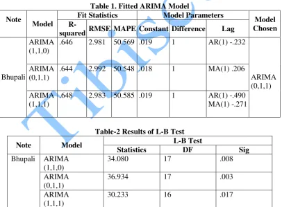
Table 1. Fitted ARIMA Model

Fit Statistics Model Parameters Note

Model R-

squared RMSE MAPE Constant Difference Lag

Model Chosen

ARIMA (1,1,0)

.646 2.981 50.569 .019 1 AR(1) -.232

ARIMA (0,1,1)

.644 2.992 50.548 .018 1 MA(1) .206 Bhupali

ARIMA (1,1,1)

.648 2.983 50.585 .019 1 AR(1) -.490 MA(1) -.271

ARIMA (0,1,1)

Table-2 Results of L-B Test L-B Test Note Model

Statistics DF Sig

ARIMA (1,1,0)

34.080 17 .008

ARIMA (0,1,1)

36.934 17 .003

Bhupali

ARIMA (1,1,1)

(8)

Fig.-1 Residual ACF and PACF plot

(9)

0 20 40 60 80 100 120 140 160

-5 0 5 10 15 20

Instance

P

it

c

h

Prediction Plot for Bhupali Note Sequence

Acual Prediction

Fig.-2 Actual versus predicted through ARIMA (0,1,1)

Conclusion

(10)

Appendix

Table 3 gives the numbers representing pitches in different octaves which will be useful in understanding the note progression of the raga in question.

Table 3: Numbers representing pitch of notes [ANO06]

C Db D Eb E F F# G Ab A Bb B

S r R g G M m P d D n N (lower octave)

-12 -11 -10 -9 -8 -7 -6 -5 -4 -3 -2 -1

S r R g G M m P d D n N (middle octave) 0 1 2 3 4 5 6 7 8 9 10 11

S r R g G M m P d D n N (higher octave)

12 13 14 15 16 17 18 19 20 21 22 23

Abbreviations: _{The letters S, R, G, M, P, D and N stand for Sa,}_Sudh_Re, Sudh Ga, Sudh Ma, Pa, Sudh Dha and Sudh Ni respectively. The letters r, g, m, d, n represent Komal Re, Komal Ga, Tibra Ma, Komal Dha and Komal

Ni respectively. Normal type indicates the note belongs to middle octave; italics implies that the note belongs to the octave just lower than the middle octave while a bold type indicates it belongs to the octave just higher than the middle octave. Sa, the tonic in Indian music, is taken at C. Corresponding Western notation is also provided. The terms “Sudh”, “Komal” and “Tibra” imply, respectively, natural, flat and sharp.

We close this section giving some general feature of raga Bhupali:-

Raga: Bhupali

Thaat (a specific way of grouping ragas according to scale): Kalyan

Aroh (ascent): S R G P, D, S

Awaroh (descent): S, D P, G, R, S

Jati: Aurabh-Aurabh (5 distinct notes allowed in ascent and 5 in descent)

Vadi Swar (most important note): G

(11)

Anga: Poorvanga pradhan (first half more important) Prakriti (nature): Restful

Pakad (catch): G, R, S, D, S R G, P G, D P G, R, S

Speciality: Meend (glide) from S to D (or S to D) and from P to G Nyas Swar (Stay notes): G, P and D

(12)

References

[ANO06] K. Adiloglu, T. Noll, K. Obermayer – A Paradigmatic Approach to Extract the melodic Structure of a Musical Piece, Journal of New Music Research, 2006, Vol. 35, no. 3, 221-236.

[BM99] J. Beran, G. Mazzola - Analyzing Musical Structure and Performance –A Statistical Approach, Statistical Science, 1999, vol. 14, no. 1, p. 47-79.

[BJ76] G.E.P. Box, G.M. Jenkins - Time Series Analysis, Forecasting and Control, San Francisco, Holden Day, 1976

[C+09a] S. Chakraborty, K. Krishnapriya, Loveleen, S. Chauhan, S.S. Solanki - Analyzing the melodic structure of a North Indian Raga: A Statistical approach, Electronic Musicological Review, Vol.XII, 2009.

[C+09b] S. Chakraborty, M. Kumari, S.S. Solanki, S. Chatterjee - On What Probability can and cannot do: A case study in Raga Malkauns, Journal of Acoustical Society of India, Vol. 36, No. 4, 2009, p. 176-180

[CS09] S. Chakraborty, R. Shukla - Raga Malkauns Revisited with Special Emphasis on Modeling, Ninad, Journal of ITC Sangeet Research Academy, Vol. 23, Dec 2009

[Dut06] D. Dutta - Sangeet Tattwa (Pratham Khanda), Brati prakashani, 5thed, 2006 (Bengali)

[D+80] D. McDowall, R. McCleary, E.E. Meidinger, R. Hay Jr. -

Interrupted time series analysis. Thousand Oaks, CA: Sage Publications, 1980