Comparing the Bidirectional Baum-Welch Algorithm and the
Baum-Welch Algorithm on Regular Lattice
Vahid Rezaei1, 4,Sima Naghizadeh2, Hamid Pezeshk3, 4, *, Mehdi Sadeghi5 and Changiz Eslahchi6
1Department of Mathematics, K.N.Toosi University of Technology. Tehran, Iran.
2The National Organization for Educational Testing (NOET), Ministry of Science, Research and Technology. 3School of Mathematics, Statistics and Computer Science, College of Science, University of Tehran, Iran.
4Bioinformatics Research Group, School of Computer Science, Institute for Research in Fundamental Sciences (IPM), Tehran, Iran.
5Department of Biophysics, National Institute of Genetic Engineering and Biotechnology, Tehran, Iran. 6Faculty of Mathematical Science, Shahid-Beheshti University, G. C., Tehran, Iran.
Received: June, 14, 2012; Accepted: August, 28, 2012
Abstract
A profile hidden Markov model (PHMM) is widely used in assigning protein sequences to protein families. In this model, the hidden states only depend on the previous hidden state and observations are independent given hidden states. In other words, in the PHMM, only the information of the left side of a hidden state is considered. However, it makes sense that considering the information of the both left and right sides of a hidden state can improve the assignment task. For this purpose, bidirectional profile hidden Markov model (BPHMM) can be used. Also, because of the evolutionary relationship between sequences in a protein family, the information of the corresponding amino acid in the preceding sequence of residues in the PHMM can be considered. For this purpose the hidden Markov random field on regular lattice (HMRFRL) is introduced. In a PHMM, the parameters are defined by the transition and emission probability matrices. The parameters are usually estimated using an EM (Expectation-Maximization) algorithm known as Baum-Welch algorithm. In this paper, the bidirectional Baum-Welch algorithm and theBaum-Welch algorithm on regular lattice are defined for estimating the parameters of the BPHMM and the HMRFRL respectively. We also compare the performance of common Welch algorithm, bidirectional Welch algorithm and the Baum-Welch algorithm on regular lattice by applying them to the real top ten protein families from Pfam database. Results show that using the lattice model for sequence assignment increases the number of correctly assigned protein sequences to profiles compared to BPHMM .
Keywords: Profile Hidden Markov Model, EM Algorithm, Bidirectional Baum-Welch Algorithm, Regular Lattice.
Introduction
A central problem in genomics is to determine functions of newly discovered proteins using the information contained in their amino acid sequences (Gribskov et al., 1987). The fundamental assumptions are that homologous protein sequences have similar functions and similar structures (Churchil1, 1989). Based on this assumption homologous sequences have
found in protein sequences (Rabiner, 1989). The PHMM is a representation of multiple sequence alignment of protein families in profiles. The five components of HMM are defined as follows (Eddy , 1998):
States: a set of states:S={S1, S2, S3,..., SN}
Emissions: a set of symbols that may be observed O= {O1,O2,...,OM}
Transition probabilities: a matrix A which its entries represent the probability of transition from hidden state si to hidden state sj:
𝑎𝑖(𝑗) = P(𝑆𝑡+1= 𝑠𝑗|𝑆𝑡 = 𝑠𝑖), 1≤ i, j ≤ N
Emission probabilities: a matrix B which its entries denote the probabilities of amino acid residue ok being emitted by state sj:
bj(k) = P(𝑂𝑡=𝑜𝑘 |𝑆𝑡 = 𝑠𝑗),1 ≤j ≤ N,1≤ k ≤ M
Initial state distribution: it is the probability that s_i is a start state:
𝜋i = P(𝑆1=𝑠𝑖),1≤ i ≤ N
In the PHMM it is assumed that the amino acid sequences are emitted from the hidden states. Note that the PHMM is specified as a triple 𝜆=( A, B, 𝜋) where A is the transition probability matrix, B is the emission probability matrix and
𝜋 is the vector of initial values. The Baum-Welch algorithm which is a special type of EM, algorithm is used for estimating these parameters (Bilmes, 1998). In the Baum-Welch algorithm it is assumed that parameters are estimated based on the information of the left side of a hidden state. But it makes sense to assume that the performance of protein recognition and assignment to PHMM's can be improved by considering information of the both sides of a hidden state. We call this the bidirectional profile hidden Markov model (BPHMM). Following Aghdam (Aghdam et al., 2010), we use the Baum-Welch algorithm twice (from left to right and right to left) or the bidirectional Baum-Welch algorithm for estimating the parameters of BPHMM.
Also, one of the major limitations in PHMM is the assumption that successive amino acid residues are independent (Rabiner, 1989). So, the probability of a protein sequence, is usually
written as the product of probabilities of amino acid residues {O1, ..., OM}, i.e.,
P(O1, O2,..., OM)= ∏ P(𝑂𝑖 𝑖)
But in protein families it is assumed that protein sequences are descended from a common ancestor (Wang and Jiang, 1994). A Multiple sequence alignment (MSA) can be used to assess the shared evolutionary origins (Just, 2001). From the resulting MSA, the phylogenetic analysis can be conducted. Many progressive alignment programs use a guild tree, which is similar to the phylogenetic tree (see Felenstein , 2004; Letunic and Bork, 2006). Using the MSA, the sequences in a protein family are arranged due to their order of evolution (Ortet and Bastein, 2010). Based on this assumption the protein sequences in the final MSA are determined by the guild tree. So, the information of the corresponding amino acid in the preceding sequence in the PHMM can be considered. We call this model the hidden Markov random field on regular lattice (HMRFRL). So, Baum-Welch algorithm on regular lattice for estimating the parameters of HMRFRL is defined. It should be noted in the HMRFRL, not only the information of the left side of a hidden state, but also the information of corresponding amino acid located above the residue in a sequence of residues should be considered.
In this paper, first both the PHMM and BPHMM are reviewed. Then the bidirectional Baum-Welch algorithm and the Baum-Baum-Welch algorithm on regular lattice for estimating the parameters of the BPHMM and HMRFRL are introduced. The necessary preliminaries including notations and extensions are presented. We show how we may modify the existing Baum-Welch algorithm to be able to use a lattice framework. Finally, we compare the results of applying both algorithms on some real data from the Pfam database (Finn et al., 2010).
Material And Method
The PHMM And BPHMM
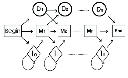
al., 1987). The PHMM is a linear structure of three states Match (M), Delete (D), and Insert (I). The number of the states must be determined by using a MSA on a protein family. Here we assume that K is the number of match states in the PHMM. So the total number of states is 3K+3. A commonly used rule is to set K equal to the number of columns including more than half of the amino acid characters (Eddy, 1998). Twenty amino acids are observed from Match and Insert states. Delete, Begin and End states are silent states because they do not emit any symbols. Following Durbin et al. (2002), using the plan 7 construction (Figure1), we estimate the transition probabilities, A, and the emission probabilities, B. This construction has no transitions from D to I, or from I to D. Figure 1 illustrates a typical PHMM. In order to improve the prediction accuracy of assigning a sequence to a PHMM, following Aghdam (Aghdam et al., 2010 ), we consider the information of the both sides of hidden states in the PHMM called bidirectional profile hidden Markov Model (BPHMM).As mentioned in section 1, in a PHMM, just the information of the left side of a hidden state e.g.ai(j) = P(St+1 = sj|St= si) is considered. So, for considering the information of the right side of a hidden state, the PHMM is conversed.These two PHMM can be integrated using a mixture density.Therefore in the BPHMM we have two PHMM and each of these PHMM has its own A and B matrices. The first PHMM is a Left to Right model (L-R-M) that considers the left to right transition between states in PHMM. The other PHMM is called (R-L-M) since the right to left transitions among states is considered. As a result, for each sequence two probabilities under L-M and R-L-M models are obtained. Using a mixture density, the probability of a sequence can be calculated by:
P(O|λ)=q1P(O| λ L-R)+q2P(O| λ R-L),
in which O denotes the sequence. q1 and q2 are
nonnegative parameters which must be estimated by an iterative process. In this paper, the both q1
and q2 are assumed to be equal to ½. However,
other non-negative values for these parameters (a weighted average) could be also admissible.λ L-R
and λ R-L indicate the parameters of L-R-M and
R-L-M models, respectively. So, the Baum-Welch algorithm is used twice for parameter estimation.
Figure 1. The Plan 7 Construction
The Bidirectional Baum-Welch Algorithm
An important question in the PHMM construction is how to estimate values of its emission probabilities (B(3K+3)×20) and transition
probabilities (A(3K+3) × (3K+3)). The Baum-Welch
algorithm is usually used for estimating parameters of PHMM. The Baum-Welch algorithm defines an iterative procedure for estimation parameters that computes maximum likelihood estimators for the unknown parameters given observation (Blims , 1998). The algorithm finds λ*=argmaxλ L(λ;O) where λ
=(A,B,π)denotes the parameters and O indicates the amino acid sequences in PHMM. The steps of Baum-Welch algorithm are as follows;
(a) Define variable γt(i) as the probability of being
in state si at time t, given the observation
sequence O1 O2 ... Ot.
γt(i)=P(St=si|O1O2...Ot)
(b) Calculate
ξt(i,j)=P(St=si,St+1=sj|O1O2...Ot)
(c) Calculate the expected number of transitions from state si to state sj by ∑ ξt t(i,j)
(d) Calculate the expected number of transitions out of state si by ∑ γt t(i)
(e) Calculate the expected number of times that an observation ok occurs in state si by
∑t.𝑜t=𝑜kγt(i)
(f) Calculate the expected frequency in state si at
Then the estimation of parameters can be found by:
𝑎̂i(j)
=Expected number of transitions from state 𝑠𝑖to state 𝑠𝑗 Expected number of transitions out of state 𝑠𝑖
= ∑ ξt t(i,j) ∑ γt t(i)
𝑏 ̂j(k) =
Expected number of times observation 𝑜𝑘 occurs in state 𝑠𝑗 Expected number of transitions out of state 𝑠𝑗
=∑t.𝑜t=𝑜kγ t(j) ∑ γt t(j)
𝜋̂i = Expected frequency of state siattime
t=1)=γ1(i).
Since the Baum-Welch algorithm finds local optima, it is important to choose initial parameters carefully. In this paper we perform the algorithm with different initial parameters in a way that the transition probabilities into Match states are larger than transition probabilities into other states.In BPHMM, the Baum-Welch algorithm is used twice for estimating the parameters. So, using a mixture density, the Baum-Welch algorithm can be defined as a Bidirectional Baum-Welch algorithm.
The Baum-Welch Algorithm On Regular Lattice
In a PHMM, only the information on the previous state of a hidden state is considered. However, in a protein family, based on the construction of protein family, the input set of query sequences is assumed to have an evolutionary relationship, by which they are descended from a common ancestor. Therefore, we propose a model which considers the effect of the evolutionary information in a sequence of amino acids, as well as the effect of the hidden state on the previous state of an amino acid. This model is a special case of a discrete state hidden Markov random field, with one point neighborhood on the lattice. This describes a special case of first order neighborhood structure. So, we can extend this model for higher order neighborhood structure e.g. a six-regular lattice with considering the following equation introduced by Besag (1974) on a regular lattice:
where njrc is the number of sites with jth
observations neighboring site (r,c),uiand vi are
parameters and isone of the amino
acids residue (multinomial data) in site (r,c). On a regular lattice the neighbors of the site with coordinates (r,c) can be denoted by {(r - 1, c), (r + 1, c),(r, c - 1),(r, c+1),(r+1,c+1), (r-1,c-1)}. This can be considered as six-regular lattice (see Rezaei et al, 2013).
In this section, for introducing the Baum-Welch algorithm on regular lattice, we need to define a new emission probability matrix by considering the information of the corresponding amino acid in the preceding sequence in the multiple sequence alignment (MSA). The MSA is a sequence alignment of three or more biological sequences such as protein, DNA, or RNA. Typically it is implied that the set of sequences share an evolutionary relationship, which means they are all descendants from a common ancestor. So, there is a relationship between phylogenies and the MSA. Phylogenetic is an area of research concerned with finding the genetic relationships between various organisms based on evolutionary relationship (Della Vedova, 2000). So, for considering the information of above amino acids, after performing an MSA on a protein family, we assume the protein sequences consisting of 21 observations (20 amino acids and one gap), are arranged in a regular lattice grid as shown by Figure 2.
So, the MSA matrix with R rows (the number of sequences) and C columns is obtained (MSAR×C).
In other words, each amino acid is arranged as a site. This matrix is called the MSA matrix, in which the site above the (r, c) is denoted by (r – 1, c). Hence, we assume each site on the lattice has a dependency with the above residue. Using the MSA matrix, we want to build a new emission probability matrix in which the size of this matrix must be the same as the emission probability matrix with 3K+3 rows and 20 columns. So, the estimation method for the new emission probability matrix, shown by β(3K+3)×20, is as
follows:
The frequencies of ordered pairs of 20 amino )
(sr,c
z m , ,..., 2 , 1 , 0 , ) exp( 1 ) exp( ) | ) ( ( 1
, j s
acids and one gap, i.e., (Or-1,c,Or,c) in each column
of MSA matrix are counted. In other words, in each column, for a given amino acid Or,c (20
amino acids), the position (r-1,c) can be filled with any of 20 types of amino acids or one gap (21 observations). So we have a 420 (20× 21) by C matrix. Dividing these frequencies by the sum of frequencies in each column the probabilities are estimated as follows:
𝛽̂i(j)=𝑃̂(Or-1,c=oj|Or,c=oi) = P
̂(𝑂r−1,c=𝑜j,𝑂r,c=𝑜𝑖) ∑j P̂(𝑂r−1,c=𝑜𝑗 ,𝑂r,c=𝑜𝑖)
1≤ j ≤ 21, 1 ≤i ≤ 20
Figure 2. Regular Lattice
This step provides us with the matrix 𝛽̂420×C.
Maximum likelihood estimators are frequently used to estimate parameters of a distribution. That is to find the parameters which makes the probability (or the chance of) observing data maximum.In the first step of construction of matrix β̂ the matrix β̂420×C is obtained. So, the
highest probability for a given amino acid Or,c,
should be chosen so that the matrix β̂420×C is
changed to matrix β̂20×C.
In each column of matrix 𝛽̂420×C, the highest
probability for a given amino acid Or,c, should be
chosen. In other words, in each column, the highest probability for each set of 21 amino acids or gap is chosen. Then the matrix 𝛽̂420×C is
changed to matrix 𝛽̂20×C.
Transposing the matrix 𝛽̂20× C , the matrix 𝛽̂C× 20is
obtained. Because we want to build a new emission probability matrix, we have to change the matrix 𝛽̂C×20 to matrix 𝛽̂(3K+3)×20. For this
purpose, we assume that the C rows consisting of Match and Insert states in which each Insert state can be repeated many times ( Figure 1). In other words, the Match states in 𝛽̂C×20 are
corresponding to Match states in 𝐵̂(3K+3)×20 and the
rows are between two Match states in βC×20
corresponding to Insert states in𝐵̂(3K+3)×20.
In the matrix 𝛽̂C×20, each row that is a Match state
should be chosen and the average values of Insert rows between two Match states are calculated. So, we have 2K Match and Insert states.
We add Delete state by using zero, so that 3K states are obtained. The average value of those rows which are before the M1 is considered as I0
state. Then the matrix 𝛽̂C×20 is changed to the
matrix 𝛽̂(3K+1)×20 with 3K+1 Match, Insert and
Delete states in rows. We add two zero rows to the 𝛽̂(3K+1)×20 as the Begin and the End states to
obtain the matrix 𝛽̂(3K+3)×20.
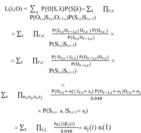
Therefore, the likelihood of parameters on a regular lattice is defined by:
L(λ;O) = ∑ P(O|S, λ)P(S|λ)𝑠 = ∑𝑠 ∏𝑟,𝑐
P(Or,c|Sr,c,Or-1,c)P(Sr,c|Sr,c-1)
= ∑𝑠 ∏𝑟,𝑐 P(𝑆r,cOr−1,c| Or,c ) P(Or,c ) P(𝑆r,cOr−1,c) ×
P(Sr,c|Sr,c-1)
= ∑𝑠 ∏𝑟,𝑐 P( Or,c | 𝑆r,c) P(Or−1,c|Or,c) P(Or−1,c) ×
P(Sr,c|Sr,c-1)
=
∑𝑠 ∏𝑜𝑖,𝑜𝑗,𝑠𝑖,𝑠𝑗 P(Or,c= oj | 𝑆r,c= 𝑠i) P(Or−1,c= 𝑜i |Or,c= 𝑜j) 0.048
× P(Sr,c= si |Sr,c-1= sj)
= ∑𝑠 ∏𝑖,𝑗
bi(𝑗)β𝑗(𝑖)
0.048 × 𝑎𝑗(𝑖) πi
(1)
where Sr,c and Or-1,c are independent, becauseSr,cjust emits Or,c. It should be noted that, in
Equation (1), P(Sr,c) and P(Or,c) on rectangular
lattice have the same meaning as P(St)$ and
P(Ot).Because there are 21 observations (20
amino acids and one gap), the P(Or-1,c) is assumed
to be equal to 1/21=0.048. Also the βj(i)'s are the
The term bi(j)βj(i)
0.048 is considered as an element of emission probability matrix on regular lattice (ERL):
ERL(i,j)= P(𝑂r,c=𝑜𝑗|𝑆r,c =𝑠𝑖,𝑂r−1,c =𝑜𝑖)
0.048 .
In other words we define the estimation of emission matrixon regular lattice (ERL) that is the entry-wise product (Hadamard product) of
𝛽̂(3K+3)×20 and𝐵̂(3K+3)×20 and divide the entries by
0.048 as follows:
𝐸𝑅𝐿̂ (3K+3)×20 =
𝛽̂(3K+3)× 20× 𝐵̂(3K+3)×20 0.048
where the ".*" is the sign of Hadamard product. Using the ERL (3K+3)×20 in common Baum-Welch
algorithm instead of and B(3K+3)×20, the
Baum-Welch algorithm on regular lattice is obtained.
Applying the Bidirectional Baum-Welch algorithm and Baum-Welch Algorithm on Regular Lattice to Real Data
In the last decades, systematic methods have been developed to assign sequence to protein families. Based on multiple sequence alignment (MSA) of protein family sequences, profile methods have
been introduced to search databases for homologous sequences. The Pfam (Finn , 2010) is a high quality set of annotated multiple alignment and pre-built profile HMM (PHMM). It is widely used to align new protein sequences on the known proteins of a given family or to recognize new member of a protein family. For each protein domain family in Pfam, there is a seed alignment which is a manually verified multiple alignment of a representative set of sequences. The Pfam database contains 11912 families (Release 24.0, October 2009). There are two components in Pfam: Pfam-A and Pfam-B. The Pfam-A entries have high quality. Given a PHMM in Pfam and a protein sequence, one can compute the probability that this protein being generated by the PHMM and infer the family that the new protein belongs to. For this purpose, the parameters of PHMM using Baum-Welch algorithm should be estimated. In this paper, using both the bidirectional Baum-Welch and the Baum-Welch algorithm on regular lattice, parameters (emission and transition matrices) are estimated and protein sequences are assigned to protein families. As shown in Table 1, we select and use ten families from top twenty protein families of Pfam-A for assignment protein sequences to protein families.
Table 1. Top ten protein families from the Pfam database
ID Accession Number of Sequences
Seed Full
RVT_1 PF00078 155 126258
WD40 PF00400 1842 101999
RVP PF00077 50 93675
Cytochrom_B_N PF00033 92 70463 HATPase_c PF02518 662 70410 BPD_transp_1 PF00528 81 70027 Oxidored_q1 PF00361 33 60333
Pkinase PF00069 54 56691
Results And Discussion
To assess the performance of our method, ten sequences from each ten families are randomly removed.We repeat this procedure10 times.Therefore, each time we have selected 100 sequences. So, in total 1000 sequences are randomly removed. Then each time we estimate the transition Matrix (A(3K+3) × (3K+3)) and the
emission matrix(B(3K+3)×20) and β(3K+3)× 20 for each
family.Therefore the estimation of parameters of BPHMM are obtained. It should be noted, the results of applying bidirectional Baum-Welch algorithm (BBWA) are compared with the results of Baum-Welch algorithm on regular lattice (BWARL) and common Baum-Welch algorithm (CBWA). In this paper due to computational challenges and round-off errors in estimating parameters, we selected just ten sequences from each family and used the .Net Framework which is a software framework that runs primarily on Microsoft Windows. In this framework the source codes of Matlab software is combined with codes of .Net.
Given ten protein families, the 1000 removed sequences are added to all families and the scores of the sequences belonging to each family based on values of estimations are computed and compared. To score a sequence and assign it to one of the top ten profiles, we use the log-odds score. It is defined by
𝑙𝑜𝑔2
prob null − prob
whereprob is the probability of sequence based on parameter estimation and null-prob is equivalent (0.05) (lengofsequence). Since there are 20
amino acids, then the probability of random occurrence of each of them is 0.05 and then for a sequence of L amino acids the probability of random occurrence is (0.05) L. The mean of the
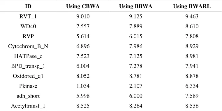
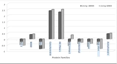
numbers of correctly assigned proteins to the top ten protein families are shown in Table 2. Based on the results shown in Table 2, the mean of correct assignment of sequences to the protein families usingBaum-Welch algorithm on regular latticeare increased in all cases.Since the Baum-Welch algorithm finds local optima, it is important to choose initial parameters carefully.So, the number of assigning sequences to original profile can be increased by choosing proper values of the initial transition and emission probability matrices. In addition to the number of correctly assigned sequences, the mean of normalized scores for each ten removed sequences in most families (8 families), using Baum-Welch algorithm on regular lattice, are more than those obtained by bidirectional Baum-Welch algorithm (Figure 3). Note that after calculating each score based on each algorithm, the average value of scores corresponding to each family are calculated. Then they are normalized. Therefore based on each algorithm the scores are different together.
Table 2. The Mean of the Numbers of Protein Sequences Assigned Correctly.
ID Using CBWA Using BBWA Using BWARL
RVT_1 9.010 9.125 9.463
WD40 7.557 7.889 8.610
RVP 5.614 6.015 7.808
Cytochrom_B_N 6.896 7.986 8.929
HATPase_c 7.523 7.125 8.981
BPD_transp_1 6.004 7.278 7.941
Oxidored_q1 8.052 8.781 8.878
Pkinase 1.034 2.107 6.334
adh_short 5.998 6.000 7.589
Not surprisingly, when we use more information due to evolutionary relationship between
sequences, the results get better.
Figure 3. The Mean of Normalized Scores for each of the Ten Removed Sequences of Each Family Using BBWA and BWARL.
Acknowledgments
Vahid Rezaei is grateful to the Department of Mathematics atK.N.Toosi University of Technology. Hamid Pezeshk would like to thankthe Department of Research Affairs of University of Tehran forfinancial support (grant number: 6103016/01/07). He is also gratefulto the Biomath Research Group at the Institute for Research inFundamental Sciences. Changiz Eslahchi is supported in partby a grant from IPM (CS-1389-0-01).
References
1.Aghdam, R., Pezeshk, H., Malekpour, S., Shemehsavar, s., Sadeghi, M., and Eslahchi C, A. (2010). Bidirectional Bayesian Mont Carlo Approach for Estimating Parameters of a Profle Hidden Markov Model. Applied Science Segment, 1(2), APS/1531
2.Besag, J.(1974). Spatial Interaction and the Statistical Analysis of Lattice Systems, Journal of the Royal Statistical Society, Series B, 36(2), 192-236
3.Bilmes, J. (1998). A Gentle Tutorial of the EM Algorithm and its Application to Parameter Estimation for Gaussian Mixture and Hidden Markov Models. International Computer Science Institute, 4-126
4.Churchill, G. (1989). Stochastic Models for Heterogeneous DNA Sequences. Bulletin of Mathematical Biology, 51(1), 79-94
5.Della Vedova, G. (2000). Multiple Sequence Alignment and Phylogenetic Reconstruction: Theory and Methods in Biological Data Analysis. PhD thesis, Citeseer
6.Durbin, R., Eddy, S., Krogh, A., and Mitchison, G. (2002). Biological Sequence Analysis. Cambridge university press Cambridge, UK:
Bioinformatics, 14(9), 755-763
8.Felsenstein, J. (2004). Inferring Phytogenies. Sunderland, Massachusetts: Sinauer Associates
9.Finn, R., Mistry, J., Tate, J., Coggill, P., Heger, A., et al. (2010). The Pfam Protein Families Database. Nucleic acids research, 38(suppl 1), D211
10.Gribskov, M., McLachlan, A., and Eisenberg, D. (1987). Profile Analysis: Detection of Distantly Related Proteins. Proceedings of the National Academy of Sciences, 84(13), 4355-4358
11.Just, W. (2001). Computational Complexity of Multiple Sequence Alignment with Sp-score. Journal of computational biology, 8(6), 615-623
12.Krogh, A., Brown, M., Mian, I., Sjolander, K., and Haussler, D. (1994). Hidden Markov Models in Computational Biology: Applications to Protein Modeling. Journal of molecular biology, 235(5), 1501-1531
13.Letunic, I. and Bork, P. (2006). Interactive Tree of Life (itol): An Online Tool for Phylogenetic Tree Display and Annotation. Bioinformatics, 23(1), 127-128
14.Ortet, P. and Bastien, O. (2010). Where Does the Alignment Score Distribution Shape Come from? Evolutionary Bioinformatics Online, 6-159
15.Pearson, W. and Sierk, M. (2005). The Limits of Protein Sequence Comparison? Current opinion in structural biology, 15(3), 254-260
16.Rabiner, L. (1989). A Tutorial on Hidden Markov Models and Selected Applications in Speech Recognition. Proceedings of the IEEE, 77(2), 257-286
17.Rezaeitabar, V., Pezeshk, H., Sadeghi, M., Eslahchi, Ch., (2013), “Assignment of Protein Sequence to Protein Profile Using Spatial Statistics”, Communications in Mathematical and in computer chemistry, 69(1), 7-24