Key words

Henryk Kordecki

_{, Maria Knapik-Kordecka}

_{Mikołaj Karmowski}

_,

Bohdan Gworys

_{, Andrzej Karmowski}

Data Dimensionality Reduction

in Anthropometrical Investigations

Redukcja wymiarowości danych

w badaniach antropometrycznych

1 _{Institute of Computer Technology, Automatics and Robotics, Wroclaw University of Technology,}

Wrocław, Poland

2 _{1st Department and Clinic of Gynecology and Obstetrics, Wroclaw Medical University, Wrocław, Poland} 3 _{Department of Angiology, Hypertension and Diabetology, Wroclaw Medical University, Wrocław, Poland} 4 _{Department of Gynecology and Obstetrics, Wroclaw Medical University, Wrocław, Poland}

5 _{Department of Anatomy, Wroclaw Medical University, Wrocław, Poland}

A – research concept and design; B – collection and/or assembly of data; C – data analysis and interpretation; D – writing the article; E – critical revision of the article; F – final approval of article; G – other

Abstract

Background. Very often it is necessary to make a decision or to establish a diagnosis on the basis of great amounts

of different kinds of data. In this paper the principal component analysis procedure was applied to anthropometri-cal data analysis.

Objectives. The aim was to simplify the process of decision making by data dimensionality reduction. A second

aim was to check how the reduction affected an analysis of the pubertal growth process.

Material and Methods. A group of 400 boys was investigated. Three main components were calculated and

inter-preted. In order to investigate growth changes, the variability of each component was approximated by fourth order polynomials.

Results. It was shown that the loss of information resulting from data dimensionality reduction is about 25%, so

the three calculated principal components contained 75% of the entire information. It seems possible to make an appropriate decision on the basis of that amount of information.

Conclusions. The results obtained fully supported using the approach presented for data analysis in the case under

consideration (Adv Clin Exp Med 2012, 21, 5, 601–606).

Key words: principal component analysis, anthropometrical data analysis, data dimensionality reduction.

Streszczenie

Wprowadzenie. Bardzo często należy podjąć decyzję lub postawić rozpoznanie na bazie dużego zbioru

różnorod-nych daróżnorod-nych. W pracy wykorzystano metodę składowych główróżnorod-nych do analizy daróżnorod-nych antropometryczróżnorod-nych.

Cel pracy. Uproszczenie procesu podejmowania danych za pomocą redukcji wymiarowości danych. Ocena

wpły-wu redukcji wymiarowości na proces analizy.

Materiał i metody. Zbadano grupę 400 chłopców. Trzy składowe główne zostały wyznaczone oraz

zinterpretowa-ne. W celu określenia parametrów wzrostu zmienność składowych była aproksymowana z wykorzystaniem wielo-mianu czwartego stopnia.

Wyniki. Pokazano, że utrata informacji w wyniku redukcji wymiarowości danych jest równa 25%, zatem 3

składo-we główne zawierają 75% całej dostępnej informacji. Wydaje się, że wykorzystując tę ilość informacji, jest możliskłado-we podjęcie prawidłowej decyzji.

Wnioski. Uzyskane rezultaty w pełni potwierdziły przydatność prezentowanego podejścia w przypadku

prezento-wanej analizy danych (Adv Clin Exp Med 2012, 21, 5, 601–606).

Słowa kluczowe: analiza składowych głównych, analiza danych antropometrycznych, redukcja wymiarowości danych.

Adv Clin Exp Med 2012, 21, 5, 601–606 ISSN 1899–5276

ORIGINAl PAPERS

The process of pubertal growth is one of the basic issues dealt with in anthropology, medicine and biology [1–5]. A relatively constant rate of de-velopment during childhood precedes the acceler-ated growth known as the pubertal growth spurt. Very often researchers have to evaluate the cor-rectness of this process in different kinds of ju-venile populations. Statistical analysis is the most common tool used for this purpose. Problems arise when the number of parameters under inves-tigation is very large. In such cases, it is very diffi-cult to make general conclusions and to interpret the results of statistical analysis. In this paper the implementation of principal component analysis (PCA) [6, 7] for data dimensionality reduction is presented. All the calculations were performed us-ing Statistica Pl software (1997, StatSoft Polska, Kraków, Poland).

Material and Methods

A group of 400 boys from lower Silesia aged 11–19 was investigated. For each individual the following 17 parameters were measured:

1. Height (B-v)

2. Sitting height (Bs-v) 3. Trunk length (sst-sy)

4. Upper extremity length (a-daIII) 5. lower extremity length (B-sy) 6. Abdominal circumference (AbdC) 7. Arm circumference (AC)

8. Thigh circumference (TC) 9. Shank circumference (SC) 10. Thoracic circumference (TrC) 11. Thoracic breadth (tl-tl) 12. Thoracic depth (xi-ts) 13. Sub-scapular skin fold (SsSF) 14. Arm skin fold (ASF)

15. Abdomen skin fold (AbdSF) 16. Hip skin fold (HSF)

17. Thigh skin fold (TSF)

Results

First, in order to simplify the calculations and the interpretation of the results, all the parameters were normalized: for each i-th value of the j-th pa-rameter the following formula was calculated [1]:

j j ij ij

X X Y

σ −

= (1)

where:

Yijis the i-th normalized value of the j-th param-eter,

Xijis the i-th value of the j-th parameter,

Xj is the average value of j-th the parameter

(sam-ple estimate), and

δj – is the standard deviation of Xj (sample esti-mate).

That way each of normalized parameters has the same variability as the original (on a differ-ent scale), the average value equals 0 and variance equals 1.

Second, the appropriate number of principal components was determined and their values were calculated.

Third, using non-linear approximation [6, 8], the variability of each principal component was es-timated and interpreted.

Determination

of the Principal Components

let YT _{= [Y}

1, Y2,...YK] be the transposed vec-tor of normalized parameters (in this case k = 17).

In order to find the first principal component P1

it is necessary to determine the vector of coeffi-cients A1T _{= [A}1

1, A12,...A1K] such that the variance of

A1T_{× Y is the maximum over all linear}

combina-tions of Y. The coefficients A should be normal-ized, which means that the constraint A1T_×A1 _{= 1}

should be fulfilled. The first principal component

P1 _{corresponds to the largest eigenvalue of}

corre-lation matrix R of vector Y, so the following equa-tion has to be solved:

|R – λ1×I| = 0 (2)

where:

R is the correlation matrix of vector Y,

λ1 is the eigenvalue vector of matrix R, and

I is the identity matrix.

The solution of Equation 2 is a set of k

eigen-values. After choosing the maximum eigenvalue λ1

it is necessary to solve the set of equations: (R – λm

1×I) ×A1 = 0 (3)

As a result, the vector of the first component coefficients A1 _{is obtained. The first principal}

com-ponent vector is given by the formula:

P1 _{= A}1

1 ×Y1 + A12 ×Y2 + ... + A1k ×Yk (4) The second component can be found by cal-culating the matrix of correlation rests R1 _{= R– A}1

× A1T _{and finding first λ}m

2 – the maximum

com-ponent of eigenvalues vector for matrix R1 – then

A2 _{– the vector of the second component}

coeffi-cients and the second component P2_{. The vectors}

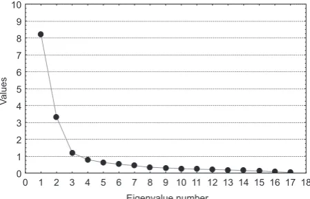
How many components should be analyzed fur-ther? There is no exact answer to this question. For the purposes of this paper, factors with eigenvalues greater than 1 were chosen [6]. Figure 1 shows the eigenvalues corresponding to k components. It can be seen that there are three components fulfilling this criterion. In Table 1 the eigenvalues, variances explained by the principal components and all cu-mulative values are shown. The principal compo-nents explain almost 75% of the variance.

The next problem was how the principal com-ponents could be interpreted. Clear interpretation is not always possible. The linear correlation co-efficients between the components and parame-ters, called component loadings, were calculated

by multiplying Ai _by m

i

λ . The greater the

cor-relation between the component and the given parameter, the more “responsible” for parame-ter changes the component is. In order to simplify component interpretation the normalized varimax rotation procedure was implemented. The values of the component loadings are given in Table 2 and shown graphically in Figure 2.

Three groups of parameters can be observed. The first five parameters are highly correlated with the first component. This set of parameters will be called the “length-height” body parameters. Param-eters 13 to 17 are highly correlated with the second component. These parameters will be called the “fatness” body parameters. Finally, a strong corre-lation may be observed between parameters 6 to 12 and the third component. This set of parameters will be called the “circumference-chest-dimension” body parameters. This way, instead of 17 parame-ters, only three easy-to-interpret principal compo-nents will be submitted to further analysis.

Fig. 1. Eigenvalues for all components

Ryc. 1. Wartości własne dla wszystkich składowych Eigenvalue number

Va

lues

0 1 2 3 4 5 6 7 8 9 10

0 1 2 3 4 5 6 7 8 9 10 11 12 13 14 15 16 17 18

Table 1. Eigenvalues, explained variances and cumulative values for three principal components Tabela 1. Wartości własne, wyjaśnione wariancje i ich wartości skumulowane

Principal component

(Główna składowa) Eigenvalue % of variance explained Cumulative eigenvalue Cumulative % of variance explained

P1 _{8.216721 48.33366 8.21672 48.33366}

P2 _{3.313781 19.49283 11.53050 67.82648}

P3 _{1.195022 7.02954 12.72552 74.85603}

Table 2. Component loading values

Tabela 2. Korelacje między zmiennymi a składowymi głównymi

Component Y1 Y2 Y3 Y4 Y5 Y6 Y7 Y8 Y9

P1 _{0.897 0.821 0.603 0.793 0.847 0.231 0.229 0.281 0.483}

P2 _{–0.04 0.014 –0.01 –0.07 –0.01 0.231 0.242 0.163 0.165}

P3 _{0.364 0.373 0.33 0.323 0.277 0.856 0.857 0.822 0.807}

Component Y10 Y11 Y12 Y13 Y14 Y15 Y16 Y17

P1 _{0.483 0.503 0.469 0.138 –0.23 –0.07 0.006 –0.50}

P2 _{0.165 0.079 0.084 0.853 0.726 0.761 0.896 0.21}

Approximation of Principal

Component Variability

The aim of this paper was to check the use-fulness of principal component analysis (PCA) for investigating body parameter changes during the pubertal growth spurt. In order to check how the variability of the principal components correlates to the known results, non-linear approximation was used [6. 9]. The variability of components as a function of the children’s age was approximated

by the least square method, using the following formula: 4 3 2 10 5 10 4 10 3 10 2 1 ) (       × +       × +       × + × + + = X B X B X B X B B X F (5) where:

X is the age of the children,

F(X) is the approximated function variability of the principal component, and

B1–B5 are function coefficients.

The reason 10 was used as the divisor was to maintain the values of coefficients B1–B5 in proximately the same range. The results of the ap-proximation are shown graphically in Figures 3, 4 and 5. The values of function F(X) coefficients and the correlation coefficients between age and components P1_{, P}2 _{and P}3 _{are presented in Table 3.}

Discussion

In individual development there are periods of intensive growth and periods of growth inhibition. One of the most intensive growth periods is the pubertal growth spurt. In this phase, the human organism attains sexual maturity and reproductive Table 3. Results of principal component variability approximation

Tabela 3. Rezultaty aproksymacji zmienności składowych głównych

Principal component (Główna składowa)

Coefficient Correlation coefficient with age

B1 B2 B3 B4 B5

P1 _{155.2895 –441.757 453.0778 –200.469 32.53778 0.59972}

P2 _{–271.360 767.0452 –793.750 357.5115 –59.3006 0.35778}

P3 _{6.360944 –20.9634 20.18564 –7.38823 0.916798 0.34739}

Fig. 2. Component loadings

Ryc. 2. Współczynniki korelacji między zmiennymi

a składowymi głównymi

F1-F5 F6-F12

F13-F17

–0.8 –0.4 0.0 0.4 0.8 0.8 0.4 1.0 0.8 0.2 –0.2 P2 P3 P1

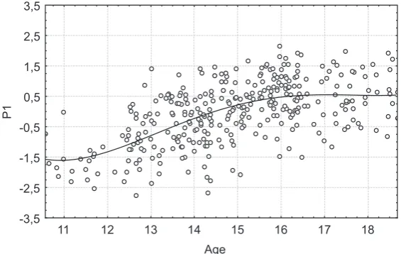
Fig. 3. Approximated variability,

principal component P1

Ryc. 3. Aproksymacja zmienności

pierwszej składowej głównej

Age P1 -3,5 -2,5 -1,5 -0,5 0,5 1,5 2,5 3,5

abilities. Physiological transformations, controlled by the neuro-hormonal system, are accompanied by deep structural changes, not only in tissues or organs but in the whole organism. Figures 3, 4 and 5 show changes in selected groups of somat-ic features during puberty.

Figure 3 illustrates the variability of the set of parameters that were called (above) “length-height” body parameters. These parameters are represented by the first principal component, P1_.

Three different phases can be observed during the pubertal growth process:

a) In the pre-pubertal phase, the beginning of pubertal growth, the velocity of “length-height” parameters growth increases (the part of the curve between 11 and 13 years of age).

b) The pubertal phase, the most intensive phase of pubertal growth, can be described as the phase when the velocity of “length-height” param-eter growth achieves its maximum (the part of the curve between 13 and 15 years of age).

c) In the post-pubertal phase, the velocity of “length-height” parameter growth decreases. At the end of this phase (the part of the curve over 17 years of age) the parameters become constant.

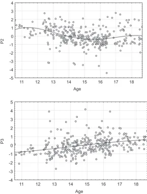
Figure 4 shows the variability of the set of

parameters represented by the second compo-nent, P2_{. This set of parameters was called (above)}

the “fatness” parameters, characterizing chang-es in the amount of fat in the body during puber-tal growth. During intensive growth the organism needs more energy and uses fat tissues as addition-al fuel. That is the explanation for the radicaddition-al de-crease in subcutaneous fat tissues as well as the of-ten observed reduction in body mass durin this period. Figure 4 provides an excellent explanation of these phenomena. Once again three phases can be specified:

a) In the pre-pubertal phase (11–13 years of age), body fat first increases, then in the middle of this phase it starts to decrease.

b) In the pubertal phase, the real growth spurt phase, reduction of body fat continues. At the end of this phase (about 15 years of age) the amount of body fat becomes stable.

c) In the post-pubertal phase (over 15 years of age), body fat slowly increases up to 18 years of age.

Figure 5 illustrates the variability of body cir-cumferences during the pubertal growth process. These parameters were called (above) “circumfer-ence-chest-dimension” parameters. The approxi-mated dependency between age and the principal

Fig. 4. Approximated variability,

principal component P2

Ryc. 4. Aproksymacja zmienności

drugiej składowej głównej

Fig. 5. Approximated variability,

principal component P3

Ryc. 5. Aproksymacja zmienności

trzeciej składowej głównej

Age

P2

-5 -4 -3 -2 -1 0 1 2 3 4

11 12 13 14 15 16 17 18

Age

P3

-4 -3 -2 -1 0 1 2 3 4 5

component representing this set of parameters is almost linear. No middle phase of pubertal growth spurt is observed. During pubertal growth, subcu-taneous fat tissue decreases and at the same time, muscle mass increases, especially in boys. Fat tissue is replaced by muscle tissue; quantitative changes are small and qualitative changes are very substan-tial. This fact explains the linear dependence be-tween age and “circumference-chest-dimension” parameters.

The purpose of this paper was to examine the possibilities of applying PCA in anthropologi-cal data investigations. The dimensionality of the problem has been reduced to three components. The approximated dependencies between age of children and components fully explained pubertal growth rules described by other authors [2, 4, 9]. The results obtained confirm the usefulness of the proposed method for data analysis in the case un-der consiun-deration.

References

[1] Bielicki T, Szklarska A, Welon Z, Malina RM: Variation in the body mass index among young adult Polish males

between 1965–1995. Int J Obes 2000, 24, 1–5.

[2] Chang T C, Robson S C, Spencer J R: Neonatal morphometric indices of fetal growth: analysis of observer

vari-ability. Early Hum Dev 1993, 35, 37–43.

[3] Charzewski J, Bielicki T: Social variation in the population of Warsaw: analysis of the height and maturity status

among 14 years old Warsaw boys. Wych Fiz Sport 1990, 38, 3–20.

[4] Kozieł S, Kołodziej H, Ulijaszek SJ: Parental education, body mass index and prevalence of obesity among

14-year-old boys between 1987 and 1997 in Wroclaw, Poland. Eur J Epidemiol 2000 16, 1163–1167.

[5] Ljung BO et al.: The secular trend in physical growth in Sweden. Ann Hum Biol 1974, 1, 3, 47–63 Philippines

1982.

[6] Berenson ML: Intermediate statistical methods and applications. Prentice-Hall Inc. 1983; pp. 308–325, 419–449. [7] Jollife IT: Principal component analysis. Springer, New York 1986.

[8] Bethea RM et al.: Statistical methods for engineers and scientists, Marcel Dekker, Inc. New York and Basel 1983,

pp. 343–351.

[9] Moreno LA, Fleta J, Sarria A, Rodriguez G, Bueno M: Secular increases in body fat percentage in male children

of Zaragoza, Spain, 1980–1995. Prev Med 2001, 33, 357–363.

Address for correspondence:

Henryk Kordecki

Institute of Computer Technology, Automatics and Robotics Wroclaw University of Technology

Wybrzeże Wyspianskiego 27 50-370 Wrocław

Poland

Tel.: +48 71 320 29 61, +48 665 224 555 E-mail: [email protected]

Conflict of interest: None declared