80
Research Journal
Volume 8, No. 23, Sept. 2014, pages 80–87
DOI: 10.12913/22998624.1120327 Research Article
Received: 2014.07.29 Accepted: 2014.08.18 Published: 2014.09.09
DETERMINANTS METHOD OF EXPLANATORY VARIABLES SET SELECTION
TO LINEAR MODEL
WitoldRzymowski1, AgnieszkaSurowiec2
1 Department of Applied Mathematics, Lublin University of Technology, Nadbystrzycka 38, 20-718 Lublin, Poland, e-mail: [email protected]
2 Department of Quantitative Methods for Management, Department of Management, Lublin University of Technology, Nadbystrzycka 38, 20-718 Lublin, Poland,, email: [email protected]
ABSTRACT
The determinants method of explanatory variables set selection to the linear model is
shown in this article. This method is very useful to find such a set of variables which
satisfy small relative error of the linear model as well as small relative error of pa-rameters estimation of this model. Knowledge of the values of the papa-rameters of this model is not necessary. An example of the use of the determinants method for world’s population model is also shown in this article. This method was tested for 224 – 1 mod-els for a set of 23 potential explanatory variables. 5 world’s population modmod-els with
one, two, three, four and five explanatory variables were chosen and analysed.
Keywords: linear regression analysis, least square parameter estimation, relative er-ror, Gram matrix.
INTRODUCTION
In this article the linear model of the form:
ε
α
α
α
α
+
+
+
+
+
=
X
X
kX
kY
0 1 1 2 2
is analyzed, where:
•
Y
is the dependent variable,•
X
1,
X
2,
,
X
k are explanatory variables.In order to initially select a set of explanatory variables for a linear model one should follow the available knowledge, experience and intuition (see [1], §1.1). Then one should take into account (see, for example [2] p. 193]) the following rec-ommendations:
A) The number of explanatory variables should not be too large.
B) Selected explanatory variables should be strongly correlated with the dependent vari-able and weakly correlated between them-selves.
C) An econometric model with selected set of ex-planatory variables should be well matched to the data.
D) The estimation parameters errors should be small.
With the exception of recommendation A, the above-mentioned recommendations are quantita-tive and there are a lot of methods, see [3], mak-ing possible to take into account at least some of these recommendations.
The main measures of the quality of the lin-ear model are: the relative error of the model, the estimation parameters relative errors and the coefficient of determination R². The most wide -spread in the Polish literature and from math-ematical point of view is a very elegant Hellwig method [4] which includes only recommenda-tion (B). Besides, using the Hellwig method, we are not able to determine whether the free pa-rameter
α
0 is needed in the model or not.More-over, the value of the coefficient of determina -tion R², more specifically the number 100R², is interpreted as a percentage of the dependent var-iable variability explained by the model. As for models without a free parameter, the inequality
1
2
>
R
is possible, then the coefficient of deter81
mination is useful only if the model contains a free parameter.
Because small estimation parameters relative errors of the model usually proclaim on the lack of collinear constraints between explanatory vari-ables, then it should be given major consideration to the recommendations made by the points (C) and (D). The error of the model (the standard de-viation of the residual component) can be calcu-lated using the determinants of two appropriate matrices, (see [3], p. 102, formula (3.76) and [5]). An interesting fact is that relative errors of estima-tion parameters can also be set using the determi-nants of two appropriate matrices and this can be done without knowledge on the values of these parameters, (see formula (14)). The formulae (12) and (14) are the basis of the determinants methods.
However, it should be pointed out that none of the methods guarantees the achievement of the right choice and the empirical verification is only the correct final evaluation of the quality of the model.
For many years the problem to create a de-mographic model to predict the world population in a fixed time range has been investigated exten -sively. Population models of living beings tend to have a form:
( )
t
t
N
f
y
t=
+
ε
t,
=
,1
2
,...
.The two oldest models: an exponential model of Malthus [6] and logistic of Verhulst [7] are the most well-known models in case of the human population. Both of these models really do not work in longer periods of time (see [8], §1.1). The models described in the works [9, 10] give a bet-ter description of the human population. But all of these models are time dependent models which are not considered in this work.
In this work an example of the use of the de-terminants method for world’s population model given by the formula:
,
40
,...
2
,1
,
, 23 23 ,
2 2 , 1 1
0
+
+
+
+
+
=
=
x
x
x
t
y
tα
α
tα
t
α
tε
tconsideration to the recommendations made by the points (C) and (D). The error of the model (the standard deviation of the residual component) can be calculated using the determinants of two appropriate matrices , see [3], p. 102, formula (3.76) and [5]. An interesting fact is that the relative errors of estimation parameters can also be set using the determinants of two appropriate matrices and it can be done without knowledge of the values of these parameters, see formula (14). The formulae (12) and (14) are the basis of the determinants methods. However, it should be pointed out that none of the methods guarantees the achievement of the right choice and the empirical verification is only the correct final evaluation of the quality of the model.
For many years the problem to create the demographic model to predict the world population in fixed time range has been investigated extensively. Population models of living beings tend to have the form:
t t Nf
yt t, 1,2,... .
The two oldest models: an exponential model of Malthus [6] and logistic of Verhulst [7] are the most well-known models in case of the human population. Both of these models really do not work in the longer periods of time (see [8], § 1.1). The models described in the works [9, 10] give a better description of the human population. But all of these models are time dependent models which are not considered in this work.
In this work an example of the use of the determinants method for world’s population model given by formula
, 40 ,... 2 , 1 , , 23 23 ,
2 2 , 1 1
0
x x x t
yt t t t t (0)
where yt is the tth observation of the world population and x1,t,x2,t,,x23,t is the tth observation of the populations in chosen countries or group of countries in year 1949t is done.
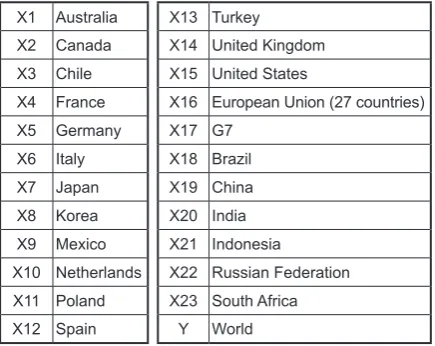
Table 1. The explanatory variables and dependent variable in world population model.
X1 Australia X13 Turkey
X2 Canada X14 United Kingdom X3 Chile X15 United States
X4 France X16 European Union (27 countries) X5 Germany X17 G7
X6 Italy X18 Brazil X7 Japan X19 China X8 Korea X20 India X9 Mexico X21 Indonesia
X10 Netherlands X22 Russian Federation X11 Poland X23 South Africa X12 Spain Y World
Of all the countries and groups of countries, available at [11], one selected only these whose population is greater than fifteen million. The Table 1 presents the list of explanatory variables and dependent variable with corresponding to them the list of selected countries in world population model.
The reason for choosing model (0) was the ease of getting a model with a potentially large number of explanatory variables. Note that the total number of set of potential explanatory variables in this case is equal to
16777215 1
224 .
The relevant calculations take into account data from the years 1950-1989 while the effects of selected models was performed in full period of 1950-2012, what can be received as a makeshift for empirical verification.
(0) where: yt is the tth observation of the world popula-tion and x1,t,x2,t,...., x23,t is the tth observation of the populations in chosen countries or group of countries in year 1949 + t is done. Of all the countries and groups of countries, available at [11], one selected only those whose population is greater than fifteen million. Table 1 presents a list of explanatory variables and de-pendent variable with alist of selected countries in
world population model corresponding to them. The reason for choosing model (0) was the ease of getting a model with a potentially large number of explanatory variables. Note that the total num-ber of set of potential explanatory variables in this case is equal to:
224 – 1 = 16777215
The relevant calculations take into account data from years 1950–1989 while the effects of selected models was performed in full period of 1950–2012, what can be received as a makeshift for empirical verification.
In view of the large number of verified mod -els it was necessary to write a computer program that performs appropriate calculations.
DETERMINANTS METHOD
Assume that
{
X
1,
X
2,...
X
k}
stands for theset of explanatory variables, where:
k
p
R
x
x
x
X
NN p p p
p
,
,1
2
,...
, 2 ,
1 ,
=
∈
=
are linear independent and the condition
N
t
y
t>
0
,
=
,1
2
,...,
is true. Taking, if necessary,
N
t
J
x
1,t=
t=
,1
=
,1
2
,...,
we can consider the models with a free param-eter. We will name „the variable” J the explana-tory variable.
Table 1. The explanatory variables and dependent var-iable in world population model
X1 Australia X13 Turkey X2 Canada X14 United Kingdom X3 Chile X15 United States
X4 France X16 European Union (27 countries) X5 Germany X17 G7
X6 Italy X18 Brazil
X7 Japan X19 China
X8 Korea X20 India X9 Mexico X21 Indonesia
X10 Netherlands X22 Russian Federation X11 Poland X23 South Africa
X12 Spain Y World
82
From the set of
{
X
1,
X
2,...
X
k}
let us choosea subset Z. In order to simplify and shorten the notations we assume that
Z
=
{
X
1,
X
2,...,
X
q}
,where
1
≤
q
≤
k
.Then we consider the model:
t t q q t t
t
x
x
x
y
=
α
1 1,+
α
2 2,+
+
α
,+
ε
,N
t
=
,1
2
,...,
, (1)whose parameters will be estimated by using Least Squares Method.
We will give the way to calculate the relative error
rel
S
(
Z
,
Y
)
of model (1) and relative errors(
Z
Y
p)
S
,
,
α
rel
of its parameters estimationα
p,p = 1,2,..., q, without determining the values of these parameters. For this purpose we will use the minors of the corresponding Gram matrix.
Least SquaresMethod – indications and
standard formulae Let:
=
Ny
y
y
Y
2 1 ,
=
Nε
ε
ε
ε
2 1 . Of course:.
,...,
2
,1
,
,
,
X
R
p
q
Y
Np
∈
=
ε
In these indications model (1) is such that:
ε
α
α
α
α
+
+
+
+
+
=
X
X
qX
qY
0 1 1 2 2
.For each: q q
R
∈
=
β
β
β
β
2 1 we define:( )
. 1 2 2 1 1∑
= = + + + = qp p p
q
qX X
X X
Y
β
β
β
β
β
Note that:
( )
( )
( )
( )
β
β
β
β
β
β
β
β
=
X
+
+
+
=
=
N q q q q N N Nx
x
x
x
x
x
x
x
x
y
y
y
Y
, 2 , 1 , 2 , 2 2 , 2 1 , 2 , 1 2 , 1 1 , 1 1 2 1...
( )
( )
( )
( )
β
β
β
β
β
β
β
β
=
X
+
+
+
=
=
N q q q q N N Nx
x
x
x
x
x
x
x
x
y
y
y
Y
, 2 , 1 , 2 , 2 2 , 2 1 , 2 , 1 2 , 1 1 , 1 1 2 1...
, (2)where:
=
N q N N q qx
x
x
x
x
x
x
x
x
, , 2 , 1 2 , 2 , 2 2 , 1 1 , 1 , 2 1 , 1 def
X
is a matrix, in which the columns are created by the coordinates of vectors
X
1,
X
2,...,
X
q.The number:
( )
21 1 ,
def 2 1 2
∑
∑
∑
= = = − = − = − N t qp p pt t
q
p pXp y x
Y Y
Y β β β
is a square of the length of the vector
( )
R
NY
Y
−
β
∈
. Estimating the parameters ofmodel (1) using the Least Squares Method we find a vector:
q q
R
∈
=
α
α
α
α
2 1 , such that:( )
2( )
2min
β
α
β
Y
Y
Y
Y
qR
−
=
−
∈ . (3)
Since:
( )
NR
R
Y
q⊂
∈
ββ
is a linear subspace of space
R
N, then exists avector
α
∈
R
q that satisfies the condition (3) andcondition
( ) ( )
Y
R
qY
Y
−
α
,
β
=
0
,
β
∈
, (4)where:
( ) ( )
,
(
( )
) ( )
1 def∑
=−
=
−
Nt t t t
y
y
y
Y
Y
Y
α
β
α
β
is Euclidean scalar product of vectors
( ) ( )
Y
R
NY
Y
−
α
,
β
∈
. Taking into account theformulae (2) and (4) we can obtain the condition:
q T
T
Y
−
X
X
α
,
β
=
0
,
β
∈
R
X
,which shows that the equation:
Y
T
T
X
X
X
α
=
(5)has a solution
α
∈
R
q. Sinceq
X
X
X
1,
2,...,
arelinearly independent, the following formula holds
83
true det
(
XTX)
>0 and consequently:(
X
TX
)
−1X
TY
=
α
(6)is the only solution of the equation (5), therefore, it is the only solution of the problem (3).
At the end of this chapter we write down the well-known formulae for relative error
rel
S
(
Z
,
Y
)
of model (1) and relative errors
rel
S
(
Z
,
Y
,
α
p)
ofits parameters estimation
α
p, p = 1,2,..., q.In order to shorten the notations certain sym-bols are introduced. Put:
∑
∑
==
N t ty
Y
1 ,
qq q q q q T b b b b b b b b b 2 1 2 22 21 1 12 11 1 XX . (7)
2 2 1 1 1 det det det , det 1 X XY X XY Z Y Z G G . (7) If
α
∈
R
q is done by formula (6), therefore,(
)
q N Y x y q N Y Z S N t qp p pt t − − = − − =
∑
∑
= = α α X 1 2 1 , 1 , (8)(
)
(
)
q N Y Y N Y Z S Y N Y Z S − − = =∑
∑
, 100 Xα100 ,
rel , (9)
At the end of this chapter we write down the well-known formulae for relative error
ZY
S ,
rel of model (1) and relative errors relS
Z,Y,p
of its parameters estimation p, qp ,12,... .
In order to shorten the notations certain symbols are introduced. Put:
N
t yt Y 1 ,
qq q q q q T b b b b b b b b b 2 1 2 22 21 1 12 11 1 XX . (7)
If Rq is done by formula 6), therefore
q N Y x y q N Y Z S N t qp p pt
t
X 1 2 1 , 1, , (8)
q N Y Y N Y Z S Y N Y Z S
, 100 X100 ,
rel , (9)
ppp pp p p b q N Y b Y Z S Y Z S
100 , 100 X ,
,
rel . (10)
2.2. Determinants method. Gram matrix G
Z,Y
.In this chapter the corresponding formulae without the values of parameters p for formulae (9) and (10) will be presented.
Let
2 2 1 2 2 2 1 2 1 2 1 2 1 q q q q q T X X X X X X X X X X X X X X X Z X X G and
2 2 1 2 1 2 2 1 2 2 2 1 2 1 2 1 2 1 , Y Y X Y X Y X Y X Y X Y X X X X X X X X X X X X X X X X Y Z q q q q q q q G ,represent Gram matrices, where
q
p p x x X
Xp p'
tN1 p,t p,'t, , ' ,12,...,
,
q
p y x Y
Xp
Nt1 p,t t , ,12,...,
.For every p ,12,...,q, the notation Gp
Z represents the matrix that was created from the matrix G
Z by removingthe pth row and the pth column, the notation
ZY
p ,
G represents the matrix that was created from the matrix G
Z,Y
by removing the last (q+1)th row and the(10)
Determinants method. Gram matrix
G
(
Z
,
Y
)
In this chapter the corresponding formulae without the values of parameters
α
p for formulae(9) and (10) will be presented. Let:
( )
= =∑
∑
∑
∑
∑
∑
∑
∑
∑
2 2 1 2 2 2 1 2 1 2 1 2 1 q q q q q T X X X X X X X X X X X X X X X Z X X G and(
)
=∑
∑
∑
∑
∑
∑
∑
∑
∑
∑
∑
∑
∑
∑
∑
∑
2 2 1 2 1 2 2 1 2 2 2 1 2 1 2 1 2 1 , Y Y X Y X Y X Y X Y X Y X X X X X X X X X X X X X X X X Y Z q q q q q q q Grepresent Gram matrices, where:
{
q
}
p
p
x
x
X
X
p p'=
∑
tN1 p,t p,'t,
,
'
∈
,1
2
,...,
∑
= ,{
q
}
p
y
x
Y
X
p=
∑
tN1 p,t t,
∈
,1
2
,...,
∑
= .For every
p
=
,1
2
,...,
q
, the notationG
p( )
Z
represents the matrix that was created from ma-trix
G
( )
Z
by removing the pth row and the pth column, the notationG
p(
Z
,
Y
)
represents thematrix that was created from the matrix
G
(
Z
,
Y
)
by removing the last (q+1)th row and the pth col-umn, the notation
G
ˆ
p(
Z
,
Y
)
represents thema-trix that was created from the mama-trix
G
( )
Z
by replacement the pth column:
∑
∑
∑
p q p pX
X
X
X
X
X
2 1by the column:
∑
∑
∑
Y
X
Y
X
Y
X
q
2 1Remark 1. In case of
q
=
1
(a model with oneexplanatory variable X) we have:
t t
t
x
y
=
α +
ε
,t
=
,1
2
,...,
N
,( )
=
∑
= N t tx
Z
1 2G
,(
)
=∑
∑
∑
∑
= = = = N t t Nt t t N
t t t N t t y x y y x x Y Z 1 2 1 1 1 2 , G ,
(
)
(
)
=
=
∑
= Nt
x
ty
tY
Z
Y
Z
1 11
,
G
ˆ
,
G
and we assume
G
1( )
Z
def=
[ ]
1
.The model errors Let us define the sets:
( )
= ≤ ≤ =∑
= qp p p p
q p X Z 1 ,..., 2 ,1 ,1 0 : β β R
( )
+ = ≤ ≤ + =∑
= + qp pXp q Y p p q
84
Number
det
G
( )
Z
is the q -dimension-al volume (q-dimensional Hausdorff meas-ure) of the parallelepipedR
( )
Z
, and number(
Z
,
Y
)
det
G
is the q+1-dimensional volume(q+1-dimensional Hausdorff measure) of the par-allelepiped
R
(
Z
,
Y
)
. Besides the parallelepiped( )
Z
R
is the base of parallelepipedR
(
Z
,
Y
)
, and numberY
−
X
α
is the height of parallelepiped(
Z
,
Y
)
R
. Therefore, we have:(
Z
Y
)
Y
X
G
( )
Z
G
,
det
det
=
−
α
. Taking into consideration the formulae (8) and (9) we get:
(
)
(
)
(
)
( )
Z
q
N
Y
Z
Y
Z
S
G
G
det
,
det
,
−
=
, (11)(
)
(
)
(
)
( )
Z
q
N
Y
Z
Y
N
Y
Z
S
G
G
det
,
det
100
,
−
=
∑
rel
. (12)Parameters estimation and estimation errors
In view of the formula (6):
( )
(
Z
)
TY
q
X
G
1 2 1 −=
=
α
α
α
α
we obtain:(
)
( )
( )
det
(
( )
)
,
,1
2
.,
,
,,
.
,
det
1
det
,
ˆ
det
1q
p
Z
Y
Z
Z
Y
Z
p pp
p
=
=
−
−G
=
G
G
G
α
p = 1,2,..., q. (13)
Remark 2. In case of model of the form
,
,...,
2
,1
,
t
N
x
y
t=
α
t=
(see Remark 1) we get:
qq q q q q T b b b b b b b b b 2 1 2 22 21 1 12 11 1 XX . (7)
2 2 1 1 1 det det det , det 1 X XY X XY Z Y Z G G . Forasmuch (see (7)):( )
( )
Z
p
q
Z
b
ppp
det
,
,1
2
,...
det
=
=
G
G
p = 1,2,..., q
then (see (11)):
(
)
(
)
(
(
)
)
( )
( )
Z
q
N
Z
Y
Z
b
Y
Z
S
Y
Z
S
p pp pG
G
G
2det
det
,
det
,
,
,
−
=
=
α
(
)
(
)
(
(
)
)
( )
( )
Z
q
N
Z
Y
Z
b
Y
Z
S
Y
Z
S
p pp pG
G
G
2det
det
,
det
,
,
,
−
=
=
α
.Now, taking into account the formulae (10) and (13), for every p = 1,2,..., q, we get
(
)
(
)
(
(
)
)
Y Z q N Y Z Y Z S pp det ,
, det 100 , , G G − =
α
rel . (14)
WORLD POPULATION MODELS
Initial set of explanatory variables
The potential explanatory variables
X
p for the model of world populationY
can be the num-bers of people in chosen countries or in groups of countries. We choseX
p presented inTa-ble 1. Therefore the considered model is of the form (1) and the relative errors
rel
S
(
Z
,
Y
)
and(
Z
Y
p)
S
,
,
α
rel
for all non-empty sets:{
J,X1,X2,...,X23}
Z⊂{J, X1, X2 ,..., X23}were determined on the basis of the data from the years 1950–1989.
The next stage, the verification, was performed for only those models with one, two, three, four and five explanatory variables out of these pre -sented in Table 1, for which none of the relative errors of parameters estimation exceeds 5%. The set of such designated models are divided into two groups: the first - the models without the free pa -rameter and the second – the models with the free parameter. Then, in each of these parts 5 mod-els with the smallest errors
rel
S
(
Z
,
Y
)
with one, two, three, four and five explanatory variables were chosen and analysed. Finally we analyse 25 models without a free parameter and 16 models with a free parameter. (In the second group there is one model with four explanatory variables and there is no model with five explanatory variables which satisfy the criterion 5% error).For each selected model we calculate the theo-retical values of world population
y
ˆ
t, t = 1,2,...,63(a full range of data from the years 1950–2012), the maximum relative errors:
3
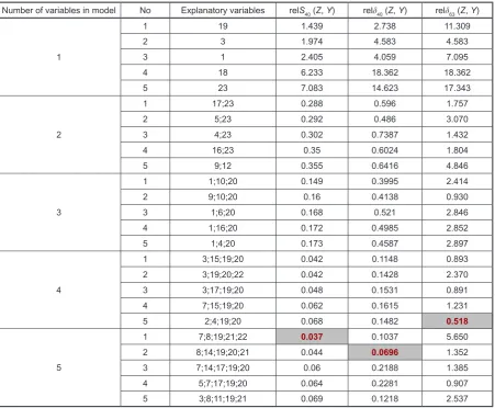
1 1;10;20 0.149 0.3995 2.414 2 9;10;20 0.16 0.4138 0.930 3 1;6;20 0.168 0.521 2.846 4 1;16;20 0.172 0.4985 2.852 5 1;4;20 0.173 0.4587 2.897
4
1 3;15;19;20 0.042 0.1148 0.893 2 3;19;20;22 0.042 0.1428 2.370 3 3;17;19;20 0.048 0.1531 0.891 4 7;15;19;20 0.062 0.1615 1.231 5 2;4;19;20 0.068 0.1482 0.518
5
1 7;8;19;21;22 0.037 0.1037 5.650 2 8;14;19;20;21 0.044 0.0696 1.352 3 7;14;17;19;20 0.06 0.2188 1.385 4 5;7;17;19;20 0.064 0.2281 0.907 5 3;8;11;19;21 0.069 0.1218 2.537
The next stage, the verification, was performed for only these models with one, two, three, four and five explanatory variables out of these presented in Table 1, for which all the relative errors of parameters estimation do not exceed 5%. The set of such designated models are divided into two groups: the first - the models without the free parameter and the second – the models with the free parameter. Then, in each of these parts 5 models with the smallest errors
Z Y
S ,
rel with one, two, three, four and five explanatory variables were chosen and analysed. Finally we analyse 25 models without the free parameter and 16 models with the free parameter. (In the second group there is one model with four explanatory variables and there is no model with five explanatory variables which satisfy the criterion 5% error).
For each selected model we calculate:
the theoretical values of world population yˆt, t1,2,...,63 (a full range of data
from the years 1950-2012),
the maximum relative errors
,
max ˆ 100%40 ,... 2 , 1 40 t t t t y y y Y
Z
rel and
,
max ˆ 100%63 ,... 2 , 1 63 t t t t y y y Y
Z
rel .
The Tables 2 and 3 show the obtained results. The Table 2 presents the results for models without the free parameters, the Table 3 presents the similar results for models with the free parameter. The numbers of explanatory variables and the relative errors for each world population linear model are presented.
Table 3. The numbers of explanatory variables and the relative errors in the world population linear model with the free parameter. The cell shaded in each errors’ column corresponds to the smallest error.
number of variables
in model No Explanatory variables relS40
Z,Y
rel
40
Z,Y
rel
63
Z,Y
1
1 0;13 0.681 1.774 1.860 2 0;9 0.686 2.095 4.167 3 0;21 0.717 3.083 3.083 4 0;23 0.885 2.177 3.564 5 0;18 1.025 2.455 4.621
2 1 2 0;1;20 0;1;23 0.202 0.210 0.558 0.517 3.187 1.760 3 0;16;20 0.263 0.475 1.421
and
3
1 1;10;20 0.149 0.3995 2.414 2 9;10;20 0.16 0.4138 0.930 3 1;6;20 0.168 0.521 2.846 4 1;16;20 0.172 0.4985 2.852 5 1;4;20 0.173 0.4587 2.897
4
1 3;15;19;20 0.042 0.1148 0.893 2 3;19;20;22 0.042 0.1428 2.370 3 3;17;19;20 0.048 0.1531 0.891 4 7;15;19;20 0.062 0.1615 1.231 5 2;4;19;20 0.068 0.1482 0.518
5
1 7;8;19;21;22 0.037 0.1037 5.650 2 8;14;19;20;21 0.044 0.0696 1.352 3 7;14;17;19;20 0.06 0.2188 1.385 4 5;7;17;19;20 0.064 0.2281 0.907 5 3;8;11;19;21 0.069 0.1218 2.537
The next stage, the verification, was performed for only these models with one, two, three, four and five explanatory variables out of these presented in Table 1, for which all the relative errors of parameters estimation do not exceed 5%. The set of such designated models are divided into two groups: the first - the models without the free parameter and the second – the models with the free parameter. Then, in each of these parts 5 models with the smallest errors
Z Y
S ,
rel with one, two, three, four and five explanatory variables were chosen and analysed. Finally we analyse 25 models without the free parameter and 16 models with the free parameter. (In the second group there is one model with four explanatory variables and there is no model with five explanatory variables which satisfy the criterion 5% error).
For each selected model we calculate:
the theoretical values of world population yˆt, t1,2,...,63 (a full range of data
from the years 1950-2012),
the maximum relative errors
,
max ˆ 100%40 ,... 2 , 1 40 t t t t y y y Y
Z
rel and
,
max ˆ 100%63 ,... 2 , 1 63 t t t t y y y Y
Z
rel .
The Tables 2 and 3 show the obtained results. The Table 2 presents the results for models without the free parameters, the Table 3 presents the similar results for models with the free parameter. The numbers of explanatory variables and the relative errors for each world population linear model are presented.
Table 3. The numbers of explanatory variables and the relative errors in the world population linear model with the free parameter. The cell shaded in each errors’ column corresponds to the smallest error.
number of variables
in model No Explanatory variables relS40
Z,Y
rel
40
Z,Y
rel
63
Z,Y
1
1 0;13 0.681 1.774 1.860 2 0;9 0.686 2.095 4.167 3 0;21 0.717 3.083 3.083 4 0;23 0.885 2.177 3.564 5 0;18 1.025 2.455 4.621
2 1 2 0;1;20 0;1;23 0.202 0.210 0.558 0.517 3.187 1.760 3 0;16;20 0.263 0.475 1.421
. Tables 2 and 3 show the obtained results. Ta-ble 2 presents the results for models without the free parameters, the Table 3 presents the simi-lar results for models with the free parameter. The numbers of explanatory variables and the
85
Table 2. The explanatory variables and the relative errors in the world population linear model without the free parameter. The cell shaded in each errors’ column corresponds to the smallest errorNumber of variables in model No Explanatory variables relS40 (Z, Y) relδ40 (Z, Y) relδ63 (Z, Y)
1
1 19 1.439 2.738 11.309
2 3 1.974 4.583 4.583
3 1 2.405 4.059 7.095
4 18 6.233 18.362 18.362
5 23 7.083 14.623 17.343
2
1 17;23 0.288 0.596 1.757
2 5;23 0.292 0.486 3.070
3 4;23 0.302 0.7387 1.432
4 16;23 0.35 0.6024 1.804
5 9;12 0.355 0.6416 4.846
3
1 1;10;20 0.149 0.3995 2.414
2 9;10;20 0.16 0.4138 0.930
3 1;6;20 0.168 0.521 2.846
4 1;16;20 0.172 0.4985 2.852
5 1;4;20 0.173 0.4587 2.897
4
1 3;15;19;20 0.042 0.1148 0.893
2 3;19;20;22 0.042 0.1428 2.370
3 3;17;19;20 0.048 0.1531 0.891
4 7;15;19;20 0.062 0.1615 1.231
5 2;4;19;20 0.068 0.1482 0.518
5
1 7;8;19;21;22 0.037 0.1037 5.650
2 8;14;19;20;21 0.044 0.0696 1.352
3 7;14;17;19;20 0.06 0.2188 1.385
4 5;7;17;19;20 0.064 0.2281 0.907
5 3;8;11;19;21 0.069 0.1218 2.537
Table 3. The numbers of explanatory variables and the relative errors in the world population linear model with the free parameter. The cell shaded in each errors’ column corresponds to the smallest error
Number of variables in model No Explanatory variables relS40 (Z, Y) relδ40 (Z, Y) relδ63 (Z, Y)
1
1 0;13 0.681 1.774 1.860
2 0;9 0.686 2.095 4.167
3 0;21 0.717 3.083 3.083
4 0;23 0.885 2.177 3.564
5 0;18 1.025 2.455 4.621
2
1 0;1;20 0.202 0.558 3.187
2 0;1;23 0.210 0.517 1.760
3 0;16;20 0.263 0.475 1.421
4 0;18;20 0.277 0.579 1.072
5 0;3;20 0.305 0.650 2.986
3
1 0;3;19;20 0.086 0.286 1.034
2 0;2;19;23 0.103 0.202 1.934
3 0;2;19;20 0.110 0.276 0.702
4 0;15;19;23 0.116 0.223 1.551
5 0;3;12;16 0.267 1.157 6.133
4 1 0;11;14;19;20 0.039 0.113 1.622
86
relative errors for each world population linear model are presented.
FINAL REMARKS
Remarks about the world population model
The maximum relative errors of all analysed models with a free parameter and one explana-tory variable do not exceed 5% (see Table 3). Among the selected models with one explanatory variable, but without free parameter there is only one such model, while the maximum relative er-rors of each of all selected models with two ex-planatory variables and free parameter also does not exceed 5%.
The models with three parameters show the greatest stability. For models without a free pa-rameter we have relδ40 ≤0.521, relδ63 ≤2.887 and for models with a free parameter we have relδ40 ≤ 0.65, relδ40 ≤3.187.
In addition, we found that among the listed models with one explanatory variable there are such whose maximum relative error in the full range of observation (t = 1, 2,..., 63) is equal to the maximum relative error in the range of adjust-ment (t = 1, 2,..., 40). These are the models with variable corresponding to the number of popula-tion in Chile and in Brazil (see Table 2) and in Indonesia (see Table 3).
It was found that in the all possible set of models (224 – 1) there is not a model with six or more parameters and theirs estimation relative er-rors not exceeding 5%.
The model without the free parameter that has the smallest error relδ63 ≈0.5%, see Table 2, con-tains variables that represent the number of
peo-Fig. 1. Comparison the China population and the world population on the basis of the data from the years 1950–2012 [11]
ple in Canada, France, China and India. In turn, the model with the free parameter that has the smallest error relδ63 ≈0.7%, see Table 3, contains variables that represent the number of people in the same countries, except France. The variables X19 and X20 that represent the number of people in China and India, are most common in both Tables 2 and 3. In addition, both of these vari-ables in both Tvari-ables 2 and 3, are present in two models with the smallest errors relδ63. It’s no sur-prising such a result, because the total number of the population of these countries is close to 37% of the world’s population. On the other hand, a comparison of the plots for China and world of population (see Fig. 1) makes this less obvious, at least in relation to variable X19.
The occurrence rarity in Tables 2 and 3 of variables X16 and X17 that represent the number of people in EU and in G7 is thought-provoking.
Not every model that is selected in accord-ance with the recommendations of the theoreti-cal procedure of the variables selection must be a good description of the studied phenomenon. An example is a model with variables {X7,X8,X19, X21, X22}, presented in Table 2.
Remarks about the determinats method
Determinants method provides an easy pro-grammable way to choose the explanatory vari-ables to any linear model even if the potential number of explanatory variables is very large.
The determinants method takes into account the quality recommendation A.
In the determinants method procedure the models which satisfy the theoretical recommen-dations B to D can be easily found.
87
REFERENCES
1. Chow G.C., Econometrics. Mc-Graw-Hill Book Company, New York 1983.
2. Zeliaś A., Pawełek B., Wanat S., Prognozowanie
ekonomiczne. Teoria. Przykłady. Zadania. PWN,
Warszawa 2003.
3. Grabiński T., Wydymus S., Zeliaś A., Metody
doboru zmiennych w modelach ekonometryc-znych. PWN, Warszawa 1982.
4. Hellwig Z., Problem optymalnego wyboru
pre-dykant. Przegląd Statystyczny, nr 3-4, 1969.
5. Kolupa M., O pewnym sposobie obliczania
współczynnika zbieżności. Przegląd Statystyczny,
nr. 1, 1975.
6. Malthus T.R., An essay on the Principal of Popula-tion. Penguin Books, 1970. Originally published in 1798.
7. Verhulst P.F., Notice sur la loi que la population suit dans son d’accroissement. Corr. Math. et Phys., vol. 10, 1838, 113–121.
8. Murray J.D., Mathematical Biology. I: An Intro-duction, Springer-Verlag, Berlin Heidelberg, 1989. (wyd. polskie: Murray J.D., Wprowadzenie do bio-matematyki. PWN, Warszawa 2006).
9. Hyb W., Kaleta J., Porównanie metod
wyznac-zania współczynników modelu matematycznego na przykładzie prognozy liczby ludności świata. Przegląd naukowy Inżynieria i Kształtowanie środowiska, vol. 2(29), 2004, 94–99.
10. Rzymowski W., Surowiec A., Method of Parameters
estimation of Pseudologistic Model. [In:] Zieliński
Z.E. (ed.), Rola informatyki w naukach
ekonom-icznych i społecznych. Innowacje i implikacje in
-terdyscyplinarne. vol. 2, Kielce 2012, 256–265. 11. http://stats.oecd.org
![Fig. 1. Comparison the China population and the world population on the basis of the data from the years 1950–2012 [11]](https://thumb-us.123doks.com/thumbv2/123dok_us/8809832.1776696/7.595.74.521.72.203/fig-comparison-china-population-world-population-basis-years.webp)
