Grammatical Differential Evolution Adaptable Particle Swarm Optimizer for Artificial Neural Network Training

(1)

a

International Journal of Electronics Communication and Computer Engineering Volume 4, Issue 1, ISSN (Online): 2249–071X, ISSN (Print): 2278–4209

Grammatical Differential Evolution Adaptable Particle

Swarm Optimizer for Artificial Neural Network

Training

Tapas Si

Department of Computer Science and Engineering Bankura Unnayani Institute of Engineering

Bankura, West Bengal, India Email: [email protected]

Abstract — In this paper, Grammatical Differential Evolution (GDE) Adaptable Particle Swarm Optimizer (GDE-APSO) is applied in training of Feed–Forward Neural Network (FNN). The error function of FNN is a highly multimodal function having too many local optima. GDE-APSO algorithm can solve multimodal function efficiently and effectively. The devised method is termed as GDE-APSO-NN and it is used to train FNN for XOR problem. Here, the CLPSO and DE/best/1/bin algorithms are also applied to train FNN for the same problem to make a comparative study. The experimental study shows that GDE-APSO performed better than CLPSO and DE/best/1/bin algorithm in FNN training.

Keywords —Grammatical Differential Evolution, Particle Swarm Optimization, CLPSO, Artificial Neural Network.

I. I

NTRODUCTION

Particle swarm optimization (PSO) [1], [2], [3] is population based global optimization algorithm having stochastic nature. PSO converges quickly but often gets stuck in local optima due to its lacks in diversity in the population. In classical PSO algorithm, particles update their position by using one velocity update equation. All the particles follow the same velocity update equation.

Tapas Si [9] devised Grammatical Differential Evolution Adaptable Particle Swarm Optimization (GDE-APSO) Algorithm in which every particle used different velocity update equations evolved by GDE.

Artificial Neural Network (ANN) [10], [11] is a useful tool is used in machine learning and applied for classification, pattern recognition, image processing etc. Different learning algorithms are used to train the ANN. Back-propagation (BP) [10] is a well-known algorithm used in ANN training. But BP algorithm has several drawbacks and they are a) getting stuck in local optima and b) slow error convergence speed. Therefore, PSO, DE etc. are used to train ANN.

B. Junyou [13] used PSO to train neural network for stock price forecasting. J . Liu and X . Qiu [14] used a combination of PSO and BP algorithm to train the neural network.Tapas Si, Simanta Hazra and N.D Jana [12] used DEGL (a variant of DE) algorithm to train FNN for classification of real world data.

The main objective of this work is to use GDE-APSO algorithm in FNN training.

Remaining of this paper is organized as follows: in Section II, particle swarm optimization and CLPSO

algorithms have been described. GDE-APSO algorithm is discussed in Section III. Feed-forward Neural Network is described in Section IV. In Section V, experimental setup is given. Results and discussions are given in Section VI. Finally conclusion with future work is given in Section.

II. P

ARTICLE

S

WARM

O

PTIMIZATION

A. Classical PSO

Each individual in PSO is called the particles. Each particle has memory to keep its personal best called pbest. The best of all pbest is called swarm’sbest or global best denoted as gbest. Particle’s position is denoted as Xifor ith index and it has velocity Vi. Each particle updates velocity by the following equation:

= + − + − (1)

=Ineria weight in the range (0, 1)

: = pbest of ithparticle : = gbest of the swarm

(0,2): = personal cognizance

(0,2): = social cognizance

= (0,1): = random number

Particles update their position by the following equation:

= + (2)

B. Comprehensive Learning PSO

J.J Liang, A.K Qin, P.N. Suganthan and S. Baskar [4] proposed Comprehensive Particle Swarm Optimizer (CLPSO). In this algorithm, each particle updates its velocity with a probability PCi for each dimension by following this equation:

=

+

−

(4)

Where

may be the other particle’s pbest or

its own pbest depending on the

probability PCi . For each ith particle, a random number is generated for each dimension and if this random number is greater than PCi, then it uses its own pbestotherwise uses other’spbest.

Comprehensive learning strategy is adopted in the following way:

1. Select two particles randomly having index r1 and r2 for ithparticle where 1 ≠ 2 ≠ .

2. Select better of them by tournament selection.

3. Winner’spbest is used as an exemplar to learn for jth

(2)

To ensure that a particle learns from good exemplars and to minimize the time wasted on poor directions, particles are allowed to learn from the exemplars until the particles causes improving for a certain number of generation called refreshing gap m and the velocity is updated using Eq.(1). After that again it learns from exemplars.

Each particle has the different PCi value in the range (0.05, 0.5) and it is calculated by the following equation:





10( 1) exp 1 1 0.05 0.45 exp(10) 1) i i NP PC    _{ }   _ _ _       

More details of CLPSO algorithm can be obtained from Ref. [4]. In the next section, GDE Adaptable PSO (GDE-APSO) algorithm is described.

III. GDE A

DAPTABLE

PSO

GDE-APSO algorithm is proposed by Tapas Si [9]. The key feature of the method is that different particles of PSO used the different velocity update equations evolved by GDE in order to create diversity in the population. Each individual in GDE represents a velocity update equation for each particle in PSO. First, all the DE individuals are initialized in such a way so that all the initial equations are valid. The DE individuals are co-evolved with the particles. DE mutation and cross-over operation are performed to generate trial solution from which velocity update equation is derived for an individual i.e. particle. If the derived equation is valid, then particle updates its velocity by using this equation. If this equation is invalid, then particle will uses velocity updating equation kept store in its memory. One advantage of this algorithm is that it reduces the number of control parameters in PSO. More specifically it is better to say that inertia weight, personal and social cognizance parameters are not required in GDE-APSO algorithm. On the other hand, it introduces scale factor, cross-over rate and number of wrapping in string derivation from the BNF grammar. Another property of GDE-APSO is that particles do not follow any topology. One disadvantage of GDE-APSO algorithm is that it consumes higher computational time than PSO, CLSPSO and DE algorithms for same population size and dimension of the problem to be optimized because genome’s length is higher than problem’s dimension. In Figure 2, the mapping from GDE individuals to particles are given. In the Figure 3, genotype-to-phenotype mapping is given.

Fig.2. Mapping from DE individual to particle in PSO

A. GDE-APSO Algorithm

1. Initialize the population of PSO and DE 2. Calculate the fitness of particles 3. Calculate the pbest and gbest 4. While termination criteria 5. For each individual

6. Perform DE mutation and crossover

7. If derived expression from DE trial vector is valid 8. Update the velocity using this new expression and

update the position 9. Else

10. Update the velocity with pbest expression and update the position

11. End

12. Calculate new fitness 13. Update pbest and gbest

14. Update velocity updating equation in its memory 15. Replace current DE vector by trial vector if it is valid

and better 16. End 17. End

B. Backus-Naur Form

The Backus-Naur Form (BNF) Grammar is used in GE for genotype-phenotype mapping. BNF is a meta-syntax used to express Context-Free Grammar (CFG) by specifying production rules in simple, human and machine --understandable manner. An example of BNF grammar is described below:

1. <expr> := (<expr><op><expr>) (0) | <var> (1)

2. <op> := + (0) |- (1) |* (2) |/ (3) 3. <var> := x1 (0)

|x2 (1) |x3 (2) |x4 (3) |r (4)

r represents a random number in the range (0,1).

C. Genotype-to-Phenotype Mapping

The DE vectors are initialized in the range [0, 255]. An example of DE individual is given in Figure 2.

Fig.3. Genotype

A mapping process is used to map from integer-value to rule number in the derivation of expression using BNF grammar by the following ways:

rule=(codon integer value) MOD (number of rules for the current non-terminal)

In the derivation process, if the current non-terminal is <expr>, then, the rule number is generated by the following way:

rule number=(172 mod 2)=0

<expr>:=(<expr><op><expr>)(172 mod 2)=0 :=(<var><op><expr>)(59 mod 2)=1 :=(x2<op><expr>) (161 mod 5)=1 :=(x2*<expr>) (86 mod 4)=2 :=(x2*<var>) (211 mod 2)=1 :=(x2*x1) (176 mod 2)=0 To ensure that a particle learns from good exemplars

and to minimize the time wasted on poor directions, particles are allowed to learn from the exemplars until the particles causes improving for a certain number of generation called refreshing gap m and the velocity is updated using Eq.(1). After that again it learns from exemplars.





10( 1) exp 1 1 0.05 0.45 exp(10) 1) i i NP PC    _{ }   _ _ _       

III. GDE A

DAPTABLE

PSO

A. GDE-APSO Algorithm

11. End

B. Backus-Naur Form

2. <op> := + (0) |- (1) |* (2) |/ (3) 3. <var> := x1 (0)

|x2 (1) |x3 (2) |x4 (3) |r (4)

C. Genotype-to-Phenotype Mapping

Fig.3. Genotype

<expr>:=(<expr><op><expr>)(172 mod 2)=0 :=(<var><op><expr>)(59 mod 2)=1 :=(x2<op><expr>) (161 mod 5)=1 :=(x2*<expr>) (86 mod 4)=2 :=(x2*<var>) (211 mod 2)=1 :=(x2*x1) (176 mod 2)=0 To ensure that a particle learns from good exemplars

and to minimize the time wasted on poor directions, particles are allowed to learn from the exemplars until the particles causes improving for a certain number of generation called refreshing gap m and the velocity is updated using Eq.(1). After that again it learns from exemplars.





10( 1) exp 1 1 0.05 0.45 exp(10) 1) i i NP PC    _{ }   _ _ _       

III. GDE A

DAPTABLE

PSO

A. GDE-APSO Algorithm

11. End

B. Backus-Naur Form

2. <op> := + (0) |- (1) |* (2) |/ (3) 3. <var> := x1 (0)

|x2 (1) |x3 (2) |x4 (3) |r (4)

C. Genotype-to-Phenotype Mapping

Fig.3. Genotype

(3)

a

When all the decoded values are used in the derivation but variables or non-terminals remain exist in the generated string, then the rule generation starts from the beginning of the genome. This process is called as

wrapping. The wrapping process may become failure

when same rule number is generated repeatedly for a variable (for an example, <expr> is replaced by (<expr><op><expr>)). Therefore it will take indefinite time. After wrapping process, if there are variables in the derived string, it is denoted as invalid and its fitness is assigned a very small value so that it can be replaced by better valid individual.

D. Differential Evolution (DE) Algorithm

Grammatical Differential Evolution (GDE) [8] is a variant of Grammatical Evolution (GE) [7] in which DE [5] algorithm used as a search engine in GDE and to generate computer programs in any arbitrary language. GE is a form of grammar based genetic programming used to generate computer program in any arbitrary language. Backus-Naur Form (BNF) grammar is used for mapping from genotype-to-phenotype. Here, genotype is real vector of fixed-length and phenotype is the derived expression from the genotype using BNF grammar.

In Classical DE [5] algorithm, a donor vector for an individual is created by perturbing a vector by the weighted difference of any other two mutual exclusive randomly selected vectors. Then the cross-over is performed between an individual and its donor vector to create a trial vector and finally if the trial solution is better than the current individual then it is replaced by the trial vector. The DE/current-to-best/1/bin [6] algorithm is used in this work.

Vi= Xi+F. (Xgbest- Xi) + F. (Xr1- Xr2)

Where Vi is the donor vector and Xi is the current solution, Xgbest is the best solution, Xr1 and Xr2 are two other vectors where r1≠ r2≠i.Here i is the index of current individual vector. The binomial cross-over is performed using the following:

for j=1:D

if rand(0,1)< CR || Jrand== j Ui(j)=Vi(j)

else Ui(j)=Xi(j) End

Here Ui is the trial vector, D is the dimension of the problem, and CR is the cross-over rate. Jrand is random index in [1, D].

E. Implementation in MATLAB

The velocity update equation can be rewritten in the following form:

( + 1) = ( ) , = 1,2,3,4 (3)

where = , = , =

,

=

The function set is F= {+,-,*, /} and the terminal

set is T= {x

1

, x

2

, x

3

, x

4

, r} where r is random constant

in (0, 1).

This is the following BNF grammar to generate MATLAB expression:

1. <expr> := <op> | <var>

2. <op> := plus (<expr>,<expr>) | minus(<expr>,<expr>) |

times (<expr>,<expr>) | pdivide (<expr>,<expr>) 3. <var>:= x1 | x2| x3|x4|r

r is a random number in (0,1)

pdivide function is defined as follows to avoid division by

zero error:

function value =pdivide(arg1,arg2) if arg2< 0.001 value=arg1; else value=arg1/arg2; end

end

In the next section, Feed-forward Neural Network

is described.

IV. F

EED

-F

ORWARD

N

EURAL

N

ETWORK

T

RAINING

Feed-Forward Neural Network is one class of neural network architecture in which input layer of source nodes projects onto computation nodes( i.e. hidden nodes or output nodes) and not vice versa. In this work, multilayer Feed-forward Neural Network is used. The Figure 4 depicts the FNN. A detail description can be obtained from [10]. In this architecture, 2 input nodes in input layer, 3 hidden nodes in hidden layer and one output node in output layer. Bias terms are used in hidden and output layers. The error function E of FNN is defined as following:

E =1_N (T − O)

where T is the target output, O is the output of the network and N is the number of input patterns. The objective of training algorithm is to minimize the training error E.

Fig.4. Multilayer Feed-forward Neural Network In this work, GDE-APSO algorithm is used to train the FNN for solving XOR problem. FNN is trained with four input-output pair : ([ 1 1]T,[0]), ([ 1 0]T,[1]), ([0 1]T,[1]), ([ 0 0]T,[0]). The synaptic weights are initialized in the range [-10, +10].

V. E

XPERIMENTAL

S

ETUP

A. Parameter Settings

(4)

(F)=0.8 and cross-over rate (CR) =0.8. The swarm size is same as population size in GDE. Refreshing gap=7, Wmax=0.9 and Wmin=0.4 in CLPSO. Vmax=0.5x (Xmax-Xmin) where [Xmin, Xmax] is the search space range. Maximum generation=400. Independent 50 runs are carried out for GDE-APSO, CLPSO and DE/best/1/bin algorithms. In GDE-APSO algorithm, initial populations are valid i.e. all initial individuals produce valid expressions.

B. PC Configuration

1. System: Fedora 17

2. CPU: AMD FX -8150 Eight-Core 3. RAM: 16 GB and

4. Software: Matlab 2010b

VI. R

ESULTS AND

D

ISCUSSIONS

GDE-APSO, CLPSO and DE/best/1/bin are applied in training of FNN for XOR problem and independent 50 runs are carried out for each. Mean and standard deviation of errors are given in Table 1. A t-test [15] has been carried out for sample size 50 with degree of freedom 98 to check the statistical significance of obtained results and t statistic has been given in Table 2.

From Table 1, it is seen that GDE-APSO-NN performed better than CLPSO-NN and DE-NN. From Table 2, it is clear that GDE-PSO-NN’s performance is statistically significant over CLPSO-NN and DE-NN because p-value of t-test is less than 0.05. GDE-APSO-NN performed better than DE-NN with higher significance than that of CLPSO-NN. GDE-APSO-NN has more robustness (i.e. always produce same results) in obtaining solutions than CLPSO-NN and DE-NN.

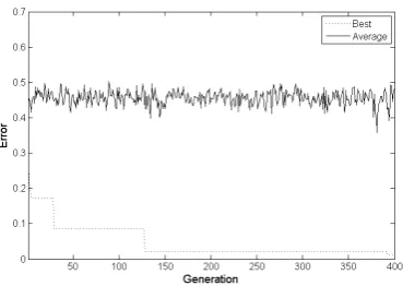
Convergence graphs are plotted in Figure 5, 6 and 7. Figure 5 depicts the explorative behavior of GDE-APSO. Figure 7 shows that all the individuals of DE quickly converge to current best solution because best/1 mutation strategy has been used in DE here. Errors of 50 runs of GDE-APSO-NN, CLPSO-NN and DE-NN are given in Figure 8, 9 and 10 respectively.

The different equations are derived in a single run are as following: minus(x3, x2)

This above expression can be written in simplified form as

= − .

‘x2’ expression can be written in simplified form as

= .

Table 1: Mean and standard deviation of errors

GDE-APSO-NN

Mean 1.17e-02

Std. Dev. 1.19e-02

CLPSO-NN Mean 1.69e-02

Std. Dev. 1.42e-02

DE-NN Mean 4.19e-02

Std. Dev. 6.18e-02

Table 2 : t-test

p-value t-value h GDE-APSO-NN

vs CLPSO 0.0487 -1.997 1

GDE-APSO-NN

vs DE-NN 0.0013 -3.3902 1

Fig.5. Convergence graph of GDE-APSO-NN

Fig.6. Convergence graph of CLPSO-NN

Fig.7. Convergence graph of DE-NN

(5)

a

Fig.9. Error of 50 runs of CLPSO-NN

Fig.10. Error of 50 runs of DE-NN

VII. C

ONCLUSION

In this paper, grammatical differential evolution adaptable particle swarm optimizer with current-to-best/1 is applied to training Feed-forward Neural Network for solving XOR problem. From this experimental study, it is seen that GDE-APSO algorithm performed better than CLPSO and DE/best/1/bin algorithm in FNN training. Future work is directed toward the application of GDE-APSO algorithm in training FNN for classification of real world data set.

R

EFERENCES

[1] R. C. Eberhart and J. Kennedy,“A new optimizer using particle

swarm theory,” In Proceedings of 6th Symposium on Micro

Machine and Human Science, Nagoya, Japan, 1995, pp. 39-43. [2] J. Kennedy and R.C. Eberhart,“Particle Swarm Optimization”, In

proceedings of IEEE Internal Conference on Neural Networks, vol. IV. Piscataway, NJ: IEEE Service Center, 1995, pp-1942-1948.

[3] Y. Shi and R. C. Eberhart, “A modified particle swarm

optimizer,” in proceedings of the IEEE congeres on Evolutionary

computation, Piscataway, NJ, 1998, pp. 69-73.

[4] J.J. Liang, A.K. Qin, P.N. Suganthan and S. Baskar,

“Comprehensive Particle Swarm Optimizer for Global Optimization of Multimodal Functions”, IEEE Transactions on Evolutionary Computation,Vol.10, No.3, June 2006, pp.281-295. [5] R. Storn and K. Price, “Dierential Evolution -A Simple and Efficient Heuristic for Global Optimization over Continuous Spaces”, Journal of Global Optimizationr,Vol. 11 , 1997, pp 341-359.

[6] Sk. Minhazul Islam, Swagatam Das, Saurav Ghose, Subhrajit Roy and P.N Suganthan, “An Adaptive Differential Evolution Algorithm With Novel Mutation and Crossover Strategies for

Global Numerical Optimization”, IEEE Transactions On Systems, Man and Cybernatics- Part B: Cybernetics, Vol. 42 Issue 2, 2012, pp.482-500.

[7] M. O'Neill, C. Ryan, “Grammatical Evolution”, IEEE Trans. Evolutionary Computation 5(4), 2001, pp.349-358.

[8] M. O'Neill, A. Brabazon,“Grammatical Differential Evolution”, In: International Conference on Artificial Intelligence (ICAI'06) CSEA Press, Las Vegas, Nevada, 2006, pp.231-236.

[9] Tapas Si, “Grammatical Differential Evolution Adaptable Particle Swarm Optimization Algorithm”, International Journal of Electronics Communication and Computer Engineering, Volume 3, Issue 6, Nov. 2012, pp. 1319-1324.

[10] Simon Haykin, Neural Networks - A Comprehensive Foundation, PHI, Second Edition,1994.

[11] X. Yao, “Evolving Artificial Neural Network”, In the Proceedings of IEEE ,Vol.87,No.9, 1999, pp.1423-1447. [12] Tapas Si, Simanta Hazra and N.D Jana, “Artificial Neural

Netwrok Training using Differential Evolutionary Algorithm”, In:Suresh Chandra Satapathy, P.S. Avadhani, Ajith Abraham (Eds.):INDIA2012, 2012,pp. 769-778.

[13] B. Junyou, “Stock Price forecasting using PSO-trained neural networks”, In proc. of IEEE Congress on Evolutionary Computation, 2007, pp.2879-2885.

[14] J. Liu and X. Qiu,“A Novel Hybrid PSO-BP Algorithm for Neural Network Training”, In proc. of International Joint Conferences on Computational Sciences and Optimization 2009, pp.300-303.

[15] N.G Das, Statistical Methods (Combined Vol) ,Tata Mcgraw Hill Education Private Limited,2008.

A

UTHOR

’

S

P

ROFILE