C. Bourdarias, S. Gerbi, Editors
MODELLING COMPRESSIBLE MULTIPHASE FLOWS
Fr´
ed´
eric Coquel
1, Thierry Gallou¨
et
2, Philippe Helluy
3, Jean-Marc
H´
erard
4, Olivier Hurisse
5and Nicolas Seguin
6Abstract. We give in this paper a short review of some recent achievements within the framework of multiphase flow modeling. We focus first on a class of compressible two-phase flow models, detailing closure laws and their main properties. Next we briefly summarize some attempts to model two-phase flows in a porous region, and also a class of compressible three-phase flow models. Some of the main difficulties arising in the numerical simulation of solutions of these complex and highly non-linear systems of PDEs are then discussed, and we eventually show some numerical results when tackling two-phase flows with mass transfer.
R´esum´e. Quelques r´esultats concernant la mod´elisation des ´ecoulements mul-tiphasiques Nous pr´esentons dans cet article quelques r´esultats r´ecents concernant la mod´elisation et la simulation num´erique des ´ecoulements multiphasiques. Nous nous con-centrons tout d’abord sur une classe de mod`eles diphasiques compressibles, en d´etaillant les lois de fermeture et les principales propri´et´es du syt`eme. Nous r´esumons ensuite bri`evement les propositions de mod´elisation d’´ecoulements diphasiques en milieu poreux et d’´ecoulements triphasiques. Quelques difficult´es apparaissant dans la simulation num´erique de ces mod`eles sont pr´esent´ees, et des r´esultats r´ecents comportant un transfert de masse entre phases sont finalement d´ecrits.
1.
Introduction
Following the initial quest of Ishii [29], the correct modelling of two-phase flows is still a widely debated topic, especially when focusing on the two-fluid approach, which aims at distinguishing mean properties of both phases (see for instance [3, 4, 7, 13, 15–18, 20, 30, 32, 36, 37]). When restrict-ing to the statistical averagrestrict-ing formalism, standard tools may be used in order to derive meanrestrict-ingful models, in order to tackle unsteady and inhomogeneous two-phase flow predictions. The present
1 CMAP, Ecole Polytechnique, UMR CNRS 7671, route de Saclay, 91128, Palaiseau cedex, France
2 LATP, Universit´e Aix-Marseille, UMR CNRS 7353, 39 rue Joliot Curie, 13453 Marseille cedex, France 3 IRMA, 7 rue Descartes, Universit´e de Strasbourg, 67084, Strasbourg, France
4 EDF, R&D, MFEE, 6 quai Watier, 78400, Chatou, France 5 EDF, R&D, MFEE, 6 quai Watier, 78400, Chatou, France
6 LJLL, Universit´e Pierre et Marie Curie,UMR CNRS 7598, Paris, France
c
EDP Sciences, SMAI 2013
paper focuses on these models, and provides some closure laws that comply with an entropy inequal-ity. The latter one is of course useful in order to control smooth and also -possibly- discontinuous solutions. One objective here is to provide a framework that might handle liquid-vapour mixtures, when the vapour phase is dilute (this corresponds to what might happen in the primary coolant circuit of nuclear power plants away from standard conditions), or when the mean flow contains a much larger amount of vapour (this may occur in the upper part of steam generators, or more likely in some severe accident configurations following the boiling crisis). Another issue is whether this framework may handle even more complex situations such as those arising when tackling three-phase flows or flows in a porous medium.
Two-fluids models require the computation of eight unknowns (statistical void fractions, mean densities, mean velocities and mean pressures). Partial differential equations may be derived for statistical void fractions, and partial mass, momentum and total energy within each phase; however, equations of state which provide the mean internal energy within each phase must be prescribed, and some closure laws are thus necessary. Actually, it is usually assumed that the averaged EOS are functions of first-order moments only (mean pressure and mean density), though this is rigor-ously valid for some specific instantaneous EOS only (such as perfect gas EOS for instance). This assumption will be kept in the present work. Even more, closure laws must be given in order to account for interfacial transfer terms. We refer the reader to the work of Kapila, Glimm and other co-workers for that difficult topic (see [4, 5, 19, 20, 31, 32]), and we only detail our methodology herein. Of course, depending on the choice of closure laws for interfacial quantities, properties of the closed set of partial differential equations may vary considerably.
Hence, the present paper aims at providing a quick review of some achievements in the framework of multiphase flow modelling. Among all constraints that should be satisfied in order to predict numerically unsteady flows containing shock patterns, the following three immediately arise:
(1) Systems are expected to be hyperbolic for all physically admissible states; (2) Smooth solutions should comply with a relevant entropy inequality;
(3) Unique jump conditions should be available in order to caracterize shock solutions.
We try to describe the basic methodology that has been considered for two-phase flow modelling of unsteady flows involving discontinuities, but we also focus in the following section on some possible extensions to the framework of flows in a porous medium and three-phase flow predictions. A short synthesis of the numerical schemes that have been developped will complete this first part. Next we will turn to some practical and recent computations, with special focus on difficulties arising when the mass transfer is accounted for.
2.
Two-phase flow modelling
Throughout the paper, αk(x, t) will denote the statistical void fraction of phase k = l, v, and
will comply with the constraintαl(x, t) +αv(x, t) = 1. Variablesρk, Uk, Pk respectively denote the
mean density, the mean velocity, the mean pressure within phase k, and we define partial masses
mk =αkρk. The total energyEkwithin phasek=l, vis defined by: Ek=ρkek(Pk, ρk) +ρk(Uk2)/2,
whereek(Pk, ρk) stands for the internal energy. The state variableW will be noted :
Thus, when neglecting the contribution of viscous effects and turbulence, the form of the governing equations of mean quantities in the two-fluid model is:
∂t(αk) +Vint(W)∂x(αk) =φk(W)
∂t(αkρk) +∂x(αkρkUk) = Γk(W)
∂t(αkρkUk) +∂x αkρkUk2
+∂x(αkPk)−Πint(W)∂x(αk) =Dk(W) + Γk(W)Uint ∂t(αkEk) +∂x(αkUk(Ek+Pk)) +Pint(W)∂t(αk) =ψk(W) +UintDk(W) + Γk(W)Hint
(1)
Contributions Γk(W),Dk(W) andψk(W) take interfacial mass transfer, drag effects and
inter-facial heat transfer into account. Besides, the termφk(W) arising in the governing equation of the
statistical void fraction αk is due to the statistical averaging [25] of the topological equation [13].
Obviously, we must enforce the following:
X
k=l,v
Γk(W) = 0 ; X
k=l,v
ψk(W) = 0 ; X
k=l,v
Dk(W) = 0 ; X
k=l,v
φk(W) = 0 . (2)
Interfacial terms
Uint= (Ul+Uv)/2 , Hint=UlUv/2 (3)
enable to account for mass and momentum transfer terms in the governing equations of mean velocities and mean total energies. Our main objective here is to determine some admissible form of all unknown quantities Γl(W), φl(W), ψl(W), Dl(W) and Πint(W), Pint(W), assuming some given
convex combination forVint(W) in terms ofUl, Uv:
Vint(W) =ξ(W)Ul+ (1−ξ(W))Uv . (4)
where ξ(W) lies in [0,1]. Physically relevant functions ξ(W) have been proposed in [7, 16], and these will be recalled at the end of this section. We also denote ck the speed of acoustic waves
within the pure k−phase, setting:
ρkc2k= (∂Pk(ek(Pk, ρk))
−1
P
k
ρk
−ρk∂ρk(ek(Pk, ρk)
2.1.
Entropy inequality
We introduce the specific entropy Sk(Pk, ρk) in each phase, which complies with:
c2k∂Pk(Sk) +∂ρk(Sk) = 0 (5)
and temperatures: 1/Tk = ∂Pk(Sk)/∂Pk(ek). We also set: µk = ek +Pk/ρk −TkSk, which is
the Gibbs potential, classically associated with the description of phase transition. We may first assume that the following constraint holds:
Πint(W)−Pint(W) = 0 (6)
and also that Πint(W) is a convex combination of both pressures, that is:
Proposition 1:
We define:
χ(W) = (1−ξ(W))/Tl[(1−ξ(W))/Tl+ξ(W)/Tv]−1 (8)
IfW denotes a smooth solution of (1), the governing equation of the entropy of the two-fluid model
η(W) =P
k=l,vmkSk may be written as follows:
∂t(η(W)) +∂x
X
k=l,v
mkUkSk
= Γl(W)(µv(W)/Tv−µl(W)/Tl)
+ Dl(W)(Uv−Ul)(1/(2Tv) + 1/(2Tl))
+ ψl(W)(Tv−Tl)/(TvTl)
+ φl(W)(Pl−Pv)(1/(2Tv) + 1/(2Tl))
The proof requires rather long calculations and is thus omitted. Obviously, when ξ(W) = 0 (or
ξ(W) = 1), one retrieves the standard Baer-Nunziato model, where the interface velocityVint(W)
corresponds to the mean velocity of the vanishing phase (see [3, 4, 32] and [17] also). This entropy budget has a straightforward counterpart in the three-dimensional framework.
• Since all quantities: Tv−Tl, Uv−Ul, Pv−Pl, µv/Tv−µl/Tl are independent quantities,
the following admissible closure laws arise:
Γl(W) =KΓ(W)(µv(W)/Tv−µl(W)/Tl),
Dl(W) =KU(W)(Uv−Ul),
ψl(W) =KT(W)(Tv−Tl),
φl(W) =KP(W)(Pl−Pv).
(9)
The first three closure laws were expected, and the last one is physically relevant: it simply means that the statistical void fraction of the liquid phase increases when the statistical pressures are such that: Pl> Pv. The -positive- scalar functions in the drag contribution
and in the heat transfer closure law may be chosen as:
KU(W) =mlmv/(ml+mv)/τU(W),
KT(W) =mlmvCl−v/(ml+mv)/τT(W),
and hence agree with the classical two-fluid litterature [29]; moreover, a relevant choice for
KP that preserves positive values of void fractions is:
KP(W) =αlαv/(Pl+Pv)/(|Pl|+|Pv|)/τP(W).
Here, τU,P,T(W) respectively denote velocity-pressure-temperature relaxation time scales.
We also set: KΓ(W) =KΓ0(W)/τΓ(W). The literature suggests physically sounded forms
forτU(W) andτT(W) on the one hand; on the other hand, accurate time scalesτP(W) can
• The closure law (8) is exactly the one that has been introduced in [7, 16]. Slightly different forms that account for the statistical void fraction gradient have been proposed later on [24], but they involve another scalar coefficient function that can hardly be determined experimentally, and are thus disregarded here. Other closure laws were proposed in [36]. Another point that is worth being emphasized is that it can be proved that the constraint (6) actually holds.
• The specific forms of Uint and Hint (see (3)) are those that guarantee that the relative
velocity Uv−Ul has no contribution in the entropy production function, when some mass
transfer occurs between phases.
• All closure laws presented above may be used for a broader class of two-fluid models [25]. The main advantage of this latter class is that it may take transition regimes into account, which is useful for the prediction of the ebulition crisis or of water-hammer situations. The approach detailed here may also be used in order to tackle the modelling of three-phase flows [23]. This particular point will be discussed in the following section.
2.2.
Main properties
We recall below the main properties of the homogeneous model associated with (1).
Property 1:
• The set of equations associated with the left-hand side of (1) has seven real eigenvalues which read:
λ1=Vint(W) (10)
λ2=Uv, λ3=Uv−cv(W), λ4=Uv+cv(W), (11)
λ5=Ul, λ6=Ul−cl(W), λ7=Ul+cl(W) (12)
Associated righteigenvectors span the whole space R7, unless |U
k−Vint(W)|/ck = 1, for
k=l, v;
• Fields associated with eigenvaluesλ2,5are linearly degenerate. Other fields associated with
eigenvalues λ3,4,6,7are genuinely nonlinear. The 1−field is linearly degenerate if:
ξ(W)(1−ξ(W)) = 0, or: ξ(W) =ml/(ml+mv) (13)
• Smooth solutions of (1) comply with the entropy inequality:
0≤∂t(η(W)) +∂x
X
k=l,v
mkUkSk
(14)
when using closure laws (9) and (8).
• Unique jump conditions hold within each isolated field for discontinuous solutions of (1) when using closure laws (13).
has been confirmed by numerous non-resonant numerical experiments [11, 18, 22, 27, 34, 38]. This is indeed a remarkable property that has only raised little attention in the two-phase flow community. We emphasize that these particular choices forξ(W) detailed in (13) are totally independent from the specific choice (8); however both formulas (13) and (8) have been considered in our overall methodology. A straightforward consequence at this stage is that the homogeneous part of system (1) is a closed set of PDE.
3.
Some extensions of the two-fluid formalism
Among all possible extensions of the two-fluid formalism that has been described above, we would like to point out at least two different situations. The first one refers to the modelling of two-phase flows in a porous region; this point was basically motivated by the need for ”component” codes in the nuclear safety framework, where the notion of porosity naturally arises when tiny obstacles in steam generators and cores are accounted for without meshing all boundaries. The second one is an innovative approach in an attempt to model three-field flows, by adopting a wider three-phase flow formalism. This is discussed in the following two subsections.
3.1.
A two-fluid model in a porous region
When the physical domain is occupied by a fluid and rigid boundaries (including walls, solid obstacles, grids,...), a possible and widely used approach consists in defining the local porosity as the ratio of the volume of fluidVf(x) over the total control volumeVtotal(x) =Vf(x) +Vs(x), where
Vs(x) stands for the volume of solid, that is:
(x) = 1− Vs(x)/Vtotal(x)
Thus, if one aims at adopting the two-fluid formalism, this leads to the problem of defining a meaningful set of PDEs, such as:
∂t() = 0
∂t(αk) +Vint(W)∂x(αk) =φk(W)
∂t(mk) +∂x(mkUk) =Γk(W)
∂t(mkUk) +∂x mkUk2
+αk∂x(Pk)−(Πint(W)−Pk)∂x(αk) =(Dk(W) + Γk(W)Uint) ∂t(αkEk) +∂x(αkUk(Ek+Pk)) +Πint(W)∂t(αk) =(ψk(W) +UintDk(W) + Γk(W)Hint)
(15) fork=l, v. The latter system enjoys similar properties such as those detailed in section 2:
Property 2:
• The homogeneous part of system (15) is hyperbolic, unless some resonance occurs if|Uk− Vint(W)|/ck= 1 or|Uk|/ck = 1; eigenvalues are:
λ0= 0 λ1=Vint(W) (16)
λ2=Uv, λ3=Uv−cv(W), λ4=Uv+cv(W), (17)
• Smooth solutions of system (15) comply with the entropy inequality:
0≤∂t(η(W)) +∂x
X
k=l,v
mkUkSk
(19)
when closure laws are defined by (8) and (9).
• Fields associated with eigenvaluesλ0= 0,λ2=Uv,λ5=Ul are linearly degenerate, and a
similar result holds forλ1=Vint(W) when the closure lawVint(W) is chosen among (13).
These results are available in [18, 24]. For practical applications in the nuclear framework, we emphasize that the resonance phenomenon is very unlikely to happen. Obviously, when sudden variations ofarise in the computational domain, there is a missing term in the momentum equation, which means in practice that results obtained with (1) are more accurate than those coming from (15), unless some singularad hocsource terms are added. Another point which is detailed in [18] is also worth being emphasized, which concerns the numerical approximation of solutions of system (15) when strong variations occur in the porous distribution (x). Actually, in that case, the computation of discontinuous solutions requires applying well-balanced schemes (with respect to the porous steady wave λ= 0), otherwise approximations obtained with colocated Finite volume schemes may converge towards wrong solutions, even if these schemes involve approximate Riemann solvers. This implies that Riemann invariants of the steady wave should be perfectly preserved.
3.2.
A class of compressible three-phase flow models
We focus now on a mixture of three phases, which will be indexed byk =l, v, s. We still use classical notations for the statistical fractionαk, the mean density, velocity and pressureρk, Uk, Pk
within each phase k, and also denote the mass fractions mk = αkρk, and the total k−energy Ek =ρkek(Pk, ρk) +ρk(Uk2)/2. The threepositive fractionsαk comply with:
Σkαk = 1
The counterpart of the two-fluid compressible model (1) is now (see [23]):
∂t(αk) +Vint(W)∂x(αk) =φ
tpf m k (W) ∂t(mk) +∂x(mkUk) = 0
∂t(mkUk) +∂x mkUk2
+∂x(αkPk) + Σj6=kΠk,j(W)∂x(αj) =D tpf m k (W) ∂t(αkEk) +∂x(αkUk(Ek+Pk))−Σj6=kΠk,j(W)∂t(αj) =Vi(W)Dtpf mk (W)
(20)
forkandj inl, v, s, when neglecting mass and energy interfacial transfer terms. Thus, closure laws
must be provided not only for φtpf mk (W) andDtpf mk (W), but also for the six unknowns Πk,l(W),
fork6=l. A first series of constraints may be written:
Σkφ tpf m
k (W) = 0;
ΣkD tpf m
k (W) = 0;
ΣkΣj6=kΠk,j(W)∂χ(αl) = 0 for: χ=x, t,
(21)
since these contributions account for interfacial transfer terms, and keeping in mind the fact that:
Moreover, it can be proved that the six unknowns Πk,j(W)uniquelydepend on the other closure
laws. Actually, introducing three functions βk(W), that represent the barycentric components of
the sole velocityVint(W) in terms of the mean phasic velocitiesUk, that is:
Vint(W) =βl(W)Ul+βv(W)Uv+βs(W)Us
and taking then into account the fact that the mixture entropy:
ηtpf m=mlSl+mvSv+msSs
should be a mathematical entropy, we eventually get that the six functions Πk,j(W) can be written
explictly in terms of the βk(W), the mean phasic pressures and temperatures Pk, Tk (see [23],
appendix G):
Πk,j(W) =πk,j(βm, Pm, Tm) with: m∈l, v, s. (23)
For instance, when choosingβv = 1 andβl=βs= 0, we get at once:
Πs,v = Πv,s= Πs,l=Ps ; Πl,v= Πv,l= Πl,s=Pl
which turns to be the counterpart of the Baer-Nunziato formalism for three-phase flows.
This is in perfect agreement with the two-phase flow formalism discussed before. It also means that the methodology can be extended to a finite number of phases N (though the algebra may become tedious when N increases). Eventually, the only remaining unknowns are the interfacial transfer termsφtpf mk (W) andDktpf m(W), but again, the entropy inequality:
0≤∂t
X
k=l,v,s
mkSk
+∂x
X
k=l,v,s
mkUkSk
(24)
provides a powerful tool in order to suggest suitable entropy-consistent closure laws for drag contri-butions between phasesDtpf mk (W), and for pressure relaxation termsφtpf mk (W). We can summarize the main properties in the following:
Property 3:
• The homogeneous part of system (20) is hyperbolic, and eigenvalues are:
λ1,2=Vint(W), (25)
λ3=Uv, λ4=Uv−cv(W), λ5=Uv+cv(W), (26)
λ6=Ul, λ7=Ul−cl(W), λ8=Ul+cl(W), (27)
λ9=Us, λ10=Us−cs(W), λ11=Us+cs(W) (28)
Resonance may occur if|Uk−Vint(W)|/ck = 1, fork=l, v, s.
• Smooth solutions of system (20) comply with the entropy inequality:
0≤∂t(η(W)) +∂x
X
k=l,v,s
mkUkSk
when applying closure laws are defined by (23) for the Πk,jand also using admissible closure
laws for interfacial transfer termsDktpf m(W), φtpf mk (W) .
• Fields associated with eigenvalues λ3 = Uv, λ6 = Ul, λ9 = Us are linearly degenerate.
If we note M = ms+mv+ml, and if we assume that either (βv, βl, βs) = (1,0,0), or:
(βv, βl, βs) = (0,1,0), or: (βv, βl, βs) = (0,0,1), or: (βv, βl, βs) = (mv/M, ml/M, ms/M),
then the field associated withλ1,2=Vint(W) is also linearly degenerate. In that case, unique
jump conditions hold field by field for solutions of system (20). The latter conditions are sufficient but not necessary (the counterpart of the proposal [25] for three-phase flows might be considered).
The reader is refered to [23] for more details.
4.
Well-suited Finite Volume schemes
We come back to two-phase flow modelling in a non-porous region, and focus on simple Finite Volume schemes that have been used for practical applications. Actually , the basic algorithm that is used to compute approximations of the whole system relies on an entropy-consistent fractional step method including an evolution step and a relaxation step. The evolution step computes approximate solutions of the pure convective system, and the relaxation step takes all source terms into account.
4.1.
Evolution step
This step computes approximate solutions of the hyperbolic homogeneous system:
∂t(αk) +Vint(W)∂x(αk) = 0 ∂t(mk) +∂x(mkUk) = 0
∂t(mkUk) +∂x mkUk2
+∂x(αkPk)−Πint(W)∂x(αk) = 0 ∂t(αkEk) +∂x(αkUk(Ek+Pk)) + Πint(W)∂t(αk) = 0
(30)
through the time interval [tn, tn+ ∆t], with given initial values Wn. The Finite Volume solver
that is used in the last section can rely on a non-conservative version of the Rusanov scheme; in that case it ensures that partial masses remain positive, and also that statistical void fractions stay in the range [0,1], provided that a specific CFL condition is enforced (see [18]). Actually, more accurate schemes such as the exact Riemann solver (see [39]), VFRoe-ncv approximate Riemann solver (see [16]), relaxation schemes (see [1, 2, 6, 10, 38]) or other schemes (see [8, 12, 33, 35, 40]) may be applied instead of the rough Rusanov scheme.
4.2.
Relaxation step
Given discrete cell values of ˜W at the beginning of each time step, we compute approximations of the coupled set of ODEs corresponding to relaxation terms, that is:
∂t(αk) =φk(W)
∂t(αkρk) = Γk(W)
∂t(αkρkUk) =Dk(W) + Γk(W)Uint
∂t(αkEk) + Πint(W)∂t(αk) =ψk(W) +UintDk(W) + Γk(W)Hint
(31)
Up to now, for a seek of simplicity and computational efficiency, all source terms have been decoupled, which means that other fractional steps are included, thus solving successively four separate steps:
∂t(αk) =δφφk(W)
∂t(αkρk) =δΓΓk(W)
∂t(αkρkUk) =δDDk(W) +δΓΓk(W)Uint
∂t(αkEk) + Πint(W)∂t(αk) =δψψk(W) +δDUintDk(W) +δΓΓk(W)Hint
(32)
associated with (δφ, δΓ, δD, δψ) equal to (1,0,0,0), (0,1,0,0), (0,0,1,0) and (0,0,0,1) respectively.
The most difficult task in the building of the Finite Volume solver is due to the mass transfer term and to the contribution φk. In particular, difficulties arise when enforcing the conservative form
for the mixture, and meanwhile requesting void fractions in the physical range [0,1] and positive densities and internal energies. Details on this part of the algorithm can be found in [26–28], and we only sketch the basic ideas below.
4.2.1. Pressure relaxation step
The pressure relaxation step computes approximations of solutions of:
∂t(αk) =φk(W)
∂t(αkρk) =∂t(αkρkUk) = 0 ∂t(αkEk) + Πint(W)∂t(αk) = 0
(33)
A ”fully implicit” discretization is applied (see [15, 26, 27]), which means that three main unknowns
α∗v, Pv∗, Pl∗ are sought, that are solutions of:
(α∗v−α0v) =α∗v(1−α∗v)(Pv∗−Pl∗)δt/τP/(Pv0+P 0 l)
(αvEv)∗−(αvEv)0+ Πint(W∗)(α∗v−α 0 v) = 0
(αvEv+ (1−αv)El)∗= (αvEv+ (1−αv)El)0
(mk)∗= (mk)0 for k=l,v
(mkUk)∗= (mkUk)0 for k=l,v
(34)
4.2.2. Gibbs potential relaxation step
In order to take mass transfer into account, we need to obtain approximations of solutions of the following system:
∂t(αk) = 0 ∂t(mk) = Γk(W) ∂t(mkUk) = Γk(W)Uint
∂t(αkEk) + Πint(W)∂t(αk) = Γk(W)Hint
(35)
A first simple scheme can be proposed in order to cope with these, that makes sense when the relaxation time step τΓ is not too small, and that preserves positive mass fractions (see [28]).
However, a more convenient and general one is the following implicit scheme:
m∗v−m0v=δtΓv(W∗)
(mvUv)∗−(mvUv)0=δtΓv(W∗)Uint(W∗)
(αvEv)∗−(αvEv)0=δtΓv(W∗)Hint(W∗)
α∗v=α0
v
(mv+ml)∗= (mv+ml)0
(αvEv+ (1−αv)El)∗= (αvEv+ (1−αv)El)0
(mlUl+mvUv)∗= (mlUl+mvUv)0
(36)
One drawback of course is that it requires solving a highly non-linear scalar equation (with respect to the unknown m∗
v), even when pure phasic equations of state are rough (such as perfect gas or
stiffened gas EOS).
5.
A few recent computational results
We start with the verification of algorithms involved in the evolution step, and then show two different two-dimensional simulations with and without mass transfer.
5.1.
One-dimensional verification results based on Riemann problems
The purpose of this subsection is to check the validity of the scheme that is used in the evolution step to predict convective effects. We consider the two-phase flow model (1), settingVint=Uv and
Πint=Pl, and we set formally:
1/τΓ(W) = 1/τP(W) = 1/τT(W) = 1/τU(W) = 0
Many Riemann problems have been considered in the verification of the evolution step, focusing either on first-order or second-order schemes. Exact solutions are computed by enforcing initial values for the left state WL, and then computing the initial right state WR =ψ(WL), where the
transformationψenables to account for all waves occuring in the solution.
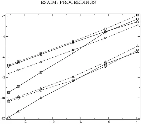
We consider here a classical 1D Riemann problem that contains only two waves: a shock wave associated with the vapour phase, and a void fraction wave associated withVint =Uv. The EOS
are assumed to be perfect gas EOS within each phase (γv = 7/5 and γl = 1.01). As it may be
checked on figure 1, which plots theL1 norm of the error with respect to the mesh size, while
con-sidering the rough first-order Rusanov scheme, the asymptotic rate of convergence ish1/2, as it can
-12 -10 -8 -6 -4 -12
-10 -8 -6 -4 -2
Figure 1. First-order Rusanov scheme : logarithm of the L1 norm of the error
||a−ah||/||a|| as a function oflog(h) for a 1D Riemann problem associated with
step (30), fora=α, Pv, Pl, Uv, Ul, ρv, ρl.
constraint isCF L= 1/2 when computing approximate solutions of the convective system. The de-tailed analysis in [10] clearly shows that the efficiency of the relaxation solver proposed in the latter reference is much higher, compared with the rough Rusanov scheme, both in terms of accuracy and CPU time for a given level of accuracy. A thorough analysis of several Riemann problems is also available in [10, 11], where authors focus on first-order and second-order schemes. The extension to second-order was achieved using a classical minmod reconstruction based on symmetrizing variables (αk, Pk, Uk, Sk) (see [9]) and a second-order Runge-Kutta time scheme. For second-order schemes,
we retrieve the expected asymptotic rate of convergence h2/3.
5.2.
Two-dimensional results without mass transfer
We consider now the two-dimensional unsteady computation of a heated wall in which a small cavity has been inserted. The model is again based on (1), while setting : Vint=Uv and Πint=Pl.
Relaxation time scales are now:
τP(W) = 10−6, τU(W) = 10−4, τT(W) = 10−6.
and 1/τΓ(W) = 0. We still use the first-order Rusanov scheme for practical computations. The
computational domain contains 105regular cells, and the CFL number is again set to 1/2.
30 millions cells). This confirms that current efforts in order to derive accurate Riemann solvers, or sufficiently large time-step schemes, are indeed mandatory.
Figure 2. Heated wall: contours of the liquid pressurePl at timeT = 0.0237.
5.3.
Three-dimensional results including mass transfer
The last test case is a preliminary result involving mass transfer between phases. We use now the relaxation scheme introduced in [38]. The implicit relaxation scheme (36) has been used in order to obtain numerical approximations. The system that is considered is still the same, though relaxation time scales are now the following:
τP(W) = 10−4, τΓ(W) = 10−4, τU(W) = 10−4, τT(W) = 10−4.
Initial conditions are also uniform in the pipe and have been set to the left inlet boundary conditions, which are:
Uvinlet=Ulinlet= 1.8281 Pvinlet=Plinlet= 55.715×10⁵ ρinletv = 28.053 ρinletl = 769.43
while setting αinletl = 0.995. Mean densities at the inlet are such that Tvinlet = Tlinlet. Both
velocity componentsVinlet
l,v andWl,vinlethave been set to zero. Two different meshes have been used,
including 60 and 500 uniform cells along the axis. We have set CF L= 0.45, thus time steps are approximately δt= 4.10−5 and δt= 5.10−6 for the coarse and the fine mesh respectively. Results
are displayed at time T = 1 on figures 3 and 4. Both velocities Ul and Uv are increasing in the
0 10 20 30 40 50 60
1,8 1,9 2 2,1 2,2
velocities
0 10 20 30 40 50 60
5,525e+06 5,53e+06 5,535e+06
pressures
0 10 20 30 40 50 60
0,992 0,994 0,996 0,998 1
liquid fraction
0 10 20 30 40 50 60
0,98 0,985 0,99 0,995 1
densities
Figure 3. Heated pipe. Pressures, velocities, normalized densities
ρk(x, T)/ρk(0, T) and liquid fraction at time T = 1. The plain line refers to
the liquid phase, whereas the dashed line represents the vapour phase. The coarse mesh contains 60 regular cells.
heated region, while densities are decreasing in the same interval. The competition of the relaxation time scales results in an increase of the liquid fraction.
6.
Conclusion
0 100 200 300 400 500 1
1,5 2 2,5 3
velocities
0 100 200 300 400 500
5,52e+06 5,53e+06 5,54e+06 5,55e+06 5,56e+06
pressures
0 100 200 300 400 500
0,992 0,994 0,996 0,998 1
liquid fraction
0 100 200 300 400 500
0,985 0,99 0,995 1
densities
Figure 4. Heated pipe. Pressures, velocities, normalized densities
ρk(x, T)/ρk(0, T) and liquid fraction at time T = 1. The plain line refers to
the liquid phase, whereas the dashed line represents the vapour phase. The fine mesh contains 500 regular cells.
systems of PDEs. Basically, four distinct requirements sustain the whole approach, which are summarized below:
• The convective part of these systems is hyperbolic unless some resonance occurs in the solution;
• Smooth solutions are in agreement with a physically meaningful entropy inequality;
• Though non-conservative first-order contributions are present in these systems, unique jump conditions can be obtained;
• Finite Volume schemes are such that numerical approximations of Riemann problems con-verge towards unique solutions even when shocks are present.
According to the authors, this is an important improvement that should help in the assessment of multiphase flow models. However, it seems mandatory to point out the following drawbacks and main challenges.
First of all, there is a lack of physical knowledge about the four relaxation time scalesτU, τP, τT, τΓ.
correct estimation ofτP thus requires further investigation and suitable experimental setups.
A second point is that these highly non-linear systems involve many different time scales that lie within a very wide range; a straightforward consequence is that high-order efficient and stable enough schemes are mandatory if one expects to get unsteady approximations that are not too far from mesh convergence. This urges the development of hybrid implicit-explicit schemes in order to obtain accurate approximations of components associated with slow internal waves. Relaxation schemes seem to provide a fair framework that might handle complex equations of state, and mean-while provide accurate enough approximations.
Another difficulty corresponds to the simulation of transitional situations such as those that may be encountered in the prediction of flows in pressurised water rectors in severe accident configura-tions.
We would like to thank PhD students Laetitia Girault, Vincent Guillemaud, Yujie Liu, Khaled Saleh for their contributions. Part of the work of Jean-Marc H´erard and Olivier Hurisse has been achieved within the framework of the NEPTUNE project, which receives financial support by CEA, EDF, AREVA and IRSN. Nicolas Seguin has been supported by LRC Manon (Mod´elisation et approximation num´erique orient´ees pour l’´energie nucl´eaire - CEA/DM2S-LJLL).
References
[1] A. Ambroso, C. Chalons, F. Coquel, T. Gali´e, Relaxation and numerical approximation of a fluid two-pressure diphasic model. ESAIM: M2AN,43 (6), pp. 1063–1097 (2009).
[2] A. Ambroso, C. Chalons, P.A. Raviart, A Godunov-type method for the seven-equation model of compressible two-phase flow, Computers and Fluids,54, pp67-91, 2012.
[3] M.R. Baer, J.W. Nunziato, A two-phase mixture theory for the deflagration to detonation transition (DDT) in reactive granular materials, IJMF,12(6), pp. 861-889, (1986).
[4] J.B. Bdzil, R. Menikoff, S.F. Son, A.K. Kapila, D.S. Stewart, Two phase modelling of deflagration to detonation transition in granular materials: a critical examination of modelling issues, Phys. of Fluids,11, pp. 378–402, (1999).
[5] W. Bo, H. Jin, D. Kim, X. Liu, H. Lee, N. Pestieau, Y. Yu, J. Glimm, J.W. Grove, Comparison and validation of multi phase closure models, Computers and mathematics with Applications,56, pp. 1291–1302, (2008). [6] C. Chalons, F. Coquel, S. Kokh, N. Spillane, Large time-step numerical scheme for the seven-equation model of
compressible two-phase flows, in proceedings of Finite Volumes for Complex Applications VI, Prague, (2011). [7] F. Coquel, T. Gallou¨et, J.M. H´erard, N. Seguin, Closure laws for a two-fluid two-pressure model, C. R. Acad.
Sci. Paris,I-332, pp. 927–932, (2002).
[8] F. Coquel, J.M. H´erard, K. Saleh, A splitting method for the isentropic Baer-Nunziato two-phase flow model, ESAIM proceedings,38, pp. 241–256 (2013).
[9] F. Coquel, J.M. H´erard, K. Saleh, N. Seguin, Two properties of two-velocity two-pressure models for two-phase flows, Communications in Mathematical Sciences, (2013).
[10] F. Coquel, J.M. H´erard, K. Saleh, N. Seguin, A robust entropy-satisfying riemann solver for the isentropic Baer-Nunziato model, submitted for publication.
[11] F. Crouzet, F. Daude, P. Galon, P. Helluy, J.M. H´erard, O. Hurisse, Y. Liu, Approximate solutions of the Baer-Nunziato model, submitted for publication, (2012).
[12] V. Deledicque, M. Papalexandris An exact Riemann solver for compressible two-phase flow models containing non-conservative products, J. Comp. Phys.,222, pp. 217-245, (2007).
[13] D.A. Drew, S.L. Passman, Theory of multi-component fluids, Applied Mathematical Sciences,135, Springer, (1999).
[15] T. Gallou¨et, P. Helluy, J.M. H´erard, J. Nussbaum, Hyperbolic relaxation models for granular flows, ESAIM: M2AN,44 (2), (2010).
[16] T. Gallou¨et, J.M. H´erard, N. Seguin, Numerical modelling of two phase flows using the two-fluid two-pressure approach, Math. Mod. Meth. in Appl. Sci.,14(5), pp. 663-700, (2004).
[17] S. Gavrilyuk, R. Saurel, Mathematical and numerical modelling of two-phase compressible flows with micro-inertia, J. Comp. Phys.,175, pp. 326-360, (2002).
[18] L. Girault, J.M. H´erard, A two-fluid hyperbolic model in a porous medium, ESAIM: M2AN,44(6), pp. 1319-1348, (2010).
[19] J. Glimm, D. Saltz, D.H. Sharp, Renormalization group solution of two-phase flow equations for Rayleigh-Taylor mixing, Phys. Letters A.,222, pp. 171–176, (1996).
[20] J. Glimm, D. Saltz, D.H. Sharp, Two-phase flow modelling of a fluid mixing layer, J. Fluid Mech., 378, pp. 119–143, (1999).
[21] S.K. Godunov , Finite difference method for numerical computation of discontinuous solutions of the equations of fluid dynamics, Mat. Sb.,47, pp. 271-300, (1959).
[22] V. Guillemaud , Mod´elisation et simulation des ´ecoulements diphasiques par une approche bifluide `a deux pressions, PhD thesis, Universit´e Aix Marseille, Marseille, France, (2007).
[23] J.M. H´erard, A three-phase flow model, Math. and Computer Model.,45, pp. 732-755, (2007).
[24] J.M. H´erard, Un mod`ele hyperbolique diphasique bifluide en milieu poreux, Comptes-Rendus M´ecanique,336, pp. 650-655, (2008).
[25] J.M. H´erard, Une classe de mod`eles diphasiques bi-fluides avec changement de r´egime, internal EDF report H-I81-2010-0486-FR, in French, (2010).
[26] J.M. H´erard, O. Hurisse, Sch´emas d’int´egration du terme de relaxation des pressions phasiques pour un mod`ele bifluide hyperbolique, EDF report H-I81-2009-01514-FR, (2009).
[27] J.-M. H´erard , O. Hurisse, A fractional step method to compute a class of compressible gas-liquid flows, Computers and Fluids,55, pp. 57-69, (2012).
[28] J.-M. H´erard , O. Hurisse, Computing two-fluid models of compressible water-vapour flows with mass transfer, AIAA paper 2012-2959, http://www.aiaa.org/ (2012).
[29] M. Ishii, Thermofluid dynamic theory of two-phase flow, Collection de la Direction des Etudes et Recherches d’Electricit´e de France, Collection Eyrolles, (1975).
[30] M. Ishii, T. Hibiki, Thermofluid dynamics of two-phase flow, Springer, (2006).
[31] H. Jin, J. Glimm, D.H. Sharp, Compressible two-pressure two-phase flow models, Physics Letters,353, pp. 469– 474, (2006).
[32] A.K. Kapila, S.F. Son, J.B. Bdzil, R. Menikoff, D.S. Stewart, Two phase modeling of a DDT: structure of the velocity relaxation zone, Phys. of Fluids,9(12), pp. 3885–3897, (1997).
[33] S. Karni , G. Hernandez-Duenas , A hybrid algorithm for the Baer Nunziato model using the Riemann invari-ants, SIAM J. of Sci. Comput.,45, pp.382-403, (2010).
[34] Y. Liu , PhD thesis, Universit´e Aix Marseille, Marseille, France, in preparation (2013).
[35] C.A. Lowe, Two-phase shock-tube problems and numerical methods of solution, J. Comp. Physics.,204, pp. 598-632, (2005).
[36] M. Papin, R. Abgrall, Fermetures entropiques pour les mod`eles bifluides `a sept ´equations, Comptes-Rendus M´ecanique,333, pp. 838-842, (2005).
[37] V. Ransom, D.L. Hicks, Hyperbolic two-pressure models for two-phase flow, J. Comp. Physics.,53, pp. 124-151, (1984).
[38] K. Saleh , Analyse et simulation num´erique par relaxation d’´ecoulements diphasiques compressibles. Contri-bution au traitement des phases ´evanescentes, PhD thesis, Universit´e Pierre et Marie Curie, Paris, France, (2012).
[39] D.W. Schwendeman, C.W. Wahle , A.K. Kapila, The Riemann problem and a high-resolution Godunov method for a model of compressible two-phase flow, J. Comp. Physics.,212, pp. 490-526, (2006).