R E S E A R C H
Open Access
A nonmonotone flexible filter method for
nonlinear constrained optimization
Ke Su
*, Xiaochuan Li and Ruyue Hou
*Correspondence: [email protected] College of Mathematics and Computer Science, Hebei University, 180 East Wusi Road, Baoding, China
Abstract
In this paper, we present a flexible nonmonotone filter method for solving nonlinear constrained optimization problems which are common models in industry. This new method has more flexibility for the acceptance of the trial step compared to the traditional filter methods, and requires less computational costs compared with the monotone-type methods. Moreover, we use a self-adaptive parameter to adjust the acceptance criteria, so that Maratos effect can be avoided a certain degree. Under reasonable assumptions, the proposed algorithm is globally convergent. Numerical tests are presented that confirm the efficiency of the approach.
MSC: Primary 90C30; secondary 65K05
Keywords: nonmonotone; filter; self-adaptive; global convergence; trust region
1 Introduction
We consider the following inequality constrained nonlinear optimization problem
(P) minf(x)
s.t.ci(x)≤, i∈I={, , . . . ,m},
wherex∈Rn, the functionsf :Rn→Randci(i∈I) :Rn→Rare all twice continuously differentiable. For convenience, letg(x) =∇f(x),c(x) = (c(x),c(x), . . . ,cm(x))TandA(x) = (∇c(x),∇c(x), . . . ,∇cm(x)). Andfkrefers tof(xk),cktoc(xk),gktog(xk) andAktoA(xk), etc.
There are various methods for solving the inequality constrained nonlinear optimization problem (P). For example, sequential quadratic programming methods, trust region ap-proaches [], penalty methods and interior point methods []. But in these works, a penalty or Lagrange function is always used to test the acceptability of the iterates. However, as we all know, there are several difficulties associated with the use of penalty function, and in particular the choice of the penalty parameter. In , Fletcher and Leyffer [] pro-posed a class of filter methods, which does not require any penalty parameter and has promising numerical results. Consequently, filter technique has employed to many ap-proaches, for instance, SLP methods [], SQP methods [, ], interior point approaches [] and derivative-free optimization [, ]. Furthermore, Fletcheret al.[] proved the global convergence of the filter-SQP method, then Ulbrich and Ulbrich [] showed its
ear local convergence. But the filter methods also encounter the Maratos effect. Marotos effect, observed by Maratos in his PhD thesis in , means some steps that make good progress toward a solution are rejected by the merit function. To overcome the drawback in filter methods, Ulbrich [] introduced a new filter method using the Lagrangian func-tion instead of the objective funcfunc-tion as the acceptance criterion. After that, Nie and Ma [] used a fixed scalar to combine the objective function and violation constraint function as one measure in the entry of the filter. But both of them used the fixed criterion to decide whether accept a trial point or not, that means the criterion is invariable no matter what improvements made by the trial point. Actually, if we can change the criterion according to the different improvements made by the current trial point, we can avoid Maratos effect to a certain degree, and decrease the computational costs as well.
On the other hand, the promising numerical results of filter methods owe to their non-monotonicity in a certain degree. Based on this property, some other non-monotone-type filter methods are proposed [–]. Gould and Toint [] also introduced a new non-monotone filter method using the area of the region inh–f plane as the criteria to decide whether a trial point is acceptable or not, whereh=h(x) is the constraint violation function andf=f(x) is the objective function at the current pointx.
Motivated by the idea and methods above, we proposed a class of nonmonotone filter trust region methods with self-adaptive parameter for solving problem (P). Our method improves previous non-monotone filter method. Unlike Ulbrich [], we do not use a La-grangian function in the filter but use the similar type of function as that in Nie and Ma []. Moreover, different from Nie and Ma [], the parameter in our method is not fixed but variable, that means the criterion is adjusted according to the different improvements. To avoid the trial point from falling into a ‘valley’, we also add the non-monotonic tech-nique into the criterion. Different from existing SQP-filter methods, we use a quadratic subproblem that always feasible to avoid the feasible restoration, hence decrease the scale of the calculation to a certain degree.
This paper is organized as follows: in Section , we introduce the feasible SQP subprob-lem and the non-monotonic flexible filter. We propose the non-monotone filter method with self-adaptive parameter in Section . Section presents the global convergence prop-erties and some numerical results are reported in Section . We end our presentation in short conclusion in Section .
2 The modified SQP subproblem and the non-monotone flexible filter method
2.1 The modified SQP subproblem
Our algorithm is an SQP method, to avoid the infeasibility of the quadratic subproblem, we choose a quadratic program that presented by Zhou []. At thekth iterate, we compute a trial step by solving the following quadratic problem,
Q(xk,Hk,ρk): mingkTd+ d
TH kd
s.t.cj(xk) +∇cj(xk)Td≤+
xk,ρk
, j∈I,
d ≤ρk,
()
where
+(xk,ρk) =max
(xk,ρk),
(xk,ρk) =min
(xk;dk) :dk ≤ρk
()
and(xk;dk) is the first order approximation to(xk+dk) =max{cj(xk+dk) :j∈I}, namely
(xk;dk) =max
cj(xk) +∇cj(xk)Tdk:j∈I
()
andρk> . We notice that these convex programs have the following properties. We can condense the above definitions by the following form
+(xk,ρk) =max
min
dk≤ρk
max j∈I
cj(xk) +∇cj(xk)Tdk
,
. ()
Lemma [] If dk= is the solution to Q(xk,Hk,ρk),then xkis a KKT point of the prob-lem(P).
Proof The proof is similar to that of Lemma . in [].
2.2 The non-monotone flexible filter with a self-adaptive parameter
In traditional filter method, originally proposed by Fletcher and Leyffer [], the accept-ability of iterates is determined by comparing the value of constraint violation and the objective function with previous iterates collected in a filter. Define the violation function h(x) byh(x) =c(x)+
∞, whereci(x)+=max{ci(x), ,i∈I}. Obviously,h(x) = if and only if xis a feasible point. So a trial point should either reduce the value of constraint violation or the objective functionf.
Definition of filter set is based on the definition of dominance as following,
Definition A pair (hk,fk) is dominated by (hj,fj) if and only ifhk≤hjandfk≤fjfor each j=k.
Definition A filter setFis a set of pairs (h,f) such that no pair dominates any other.
To ensure the convergence, some additional conditions are required to decide whether to accept a trial point to the filter or not. The traditional acceptable criterion is as follow-ing.
Definition A trial pointxis called acceptable to the filter if and only if
either h(x)≤βhj or f(x)≤fj–γhj for∀(hj,fj)∈F, ()
where <γ <β< are constants. In practice,βis close to andγ close to .
Actually, in traditional filter method, some good point such as superlinear convergent step may be rejected due to the increase of both objective function value and constraint violation value compared to other entries in filter. That is the reason why the Maratos effect occurs. So motivated by [], we substitute the original objective functionf(xk) at thekth iterate by the following function
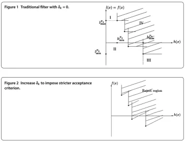
Figure 1 Traditional filter withδk= 0.
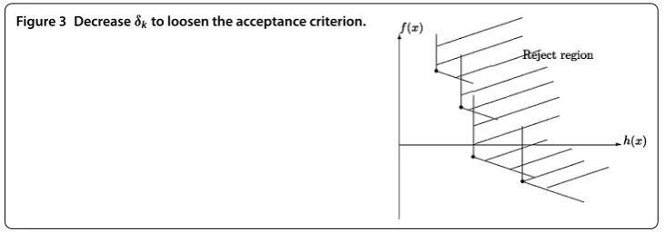
Figure 2 Increaseδkto impose stricter acceptance
criterion.
whereci(xk)+=max{ci(xk), }fori= , , . . . ,m. Hereδkis a self-adaptive parameter atkth iterate, it can be changed according to the different improvements that made by the cur-rent trial point. Note that the traditional filter methods are the special cases withδk= , and we hope overcome the Maratos effect with suitableδk.
We aim to reduce the value of bothh(x) andl(x). By original criterion, the trial point is acceptable if and only if () holds. Nie and Ma [] proposed a trust region filter method with a given penalty parameter which is negative, but in this paper, different from [], the parameterδkis a variable scalar which is changed according to the different improve-ments caused by the trial point. Specifically, at the beginning, letδ= , that is what the traditional filter method does, andf(xk) =l(xk) (see Figure ).
There are four regions in the right-hand half space I, II, III, IV. At the current iteratek, if the trial pointxkmoves into the region IV, that means the pair (hk,lk) is located in region IV, we say that the trial point is rejected according to our criterion. Ifxkmoves into the region I, II, or III, we accept it, but need to adjust the parameterδk in the criterion. For region III, we say that the algorithm does not make a good improvement, since we do not want to accept points with larger constraint violation. Thus we intent to impose stricter acceptance criterion, that means to increase the value ofδk, which will result in the bigger reject area and smaller acceptable area (see Figure ). So updateδkas following:
δk+=min ρk,δk+ lk–lk+
hk–h+k
. ()
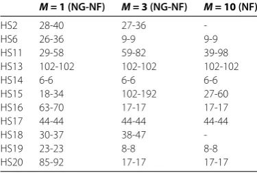
Figure 3 Decreaseδkto loosen the acceptance criterion.
area bigger (see Figure ). So updateδkas following:
δk+=max –ρk,δk– lk–l+k
hk–h+k
. ()
Ifxkmoves into region I, we will also accept it because the value of constraint violation does decrease, and we can also accept the increase ofl(xk) in finite steps. Meanwhile, the value ofδkwill not be changed. Ifxkmoves into region IV, that means this trial point is rejected, andδkalso should be remained in the next iterate.
As we all know, because of the non-monotone properties of filter method in a certain degree, it has the good numerical results. Su and Pu [] also proposed a modified non-monotone filter method to exhibit a further non-non-monotone technique. Motivated by this, we loosen the acceptance criterion by non-monotonic technique and give the following criteria.
Definition A pointxis acceptable to the filter if and only if
h(x)≤β max
≤r≤m(k)–hk–r or l(x)≤max
lk, m(k)–
r=
λkrlk–r
–γh(x), ()
where (hk–r,lk–r)∈Ffor ≤r≤m(k) – , and ≤m(k)≤min{m(k– ) + ,M},M≥ is a given positive constant,mr=(k)–λkr= ,λkr∈(, ) and there exists a positive constantλ such thatλkr≥λ.
Similar to the traditional filter methods, we also need to update the filter setFat each successful iteration, the technique is equivalent to the traditional method with the modi-fied acceptance rule ().
To control the infeasibility, an upper bound condition of violation function is needed, namelyh(x)≤u, whereuis a positive scalar, which can be implemented in the algorithm by initiating the filter with the pair (u, –∞).
3 A nonmonotone flexible filter algorithm
At the currentkth iterate, the trial pointxkis accepted by our algorithm if it satisfies two conditions, first is accepted by the filter set, second is sufficiently reduction. We define the sufficient reduction condition is as following:
whereα,αare constants, the relaxed actual reduction raredlkand the predicted reduction predfkare defined as
raredlk=l(xk+dk) –max
l(xk), m(k)–
r=
λkrlk–r
, ()
predfk= –gkTdk– d
T
kHkdk, ()
hl(k)= max
≤r≤m(k)–hk–r ()
and the matrixHkis the Hessian matrix∇f(xk) or an approximate to it,mr=(k)–λkr= ,
λkr∈(, ), ≤m(k)≤min{m(k– ) + ,M},M≥ is a given positive constant. A formal description of the algorithm is given as follows.
Algorithm A
Step. Let <ρ< , <γ <β< , <λ≤, <γ<γ≤ <γ,M≥,u> ,α=α= .. Choose an initial pointx∈Rn, a symmetric matrixH∈Rn×nand an initial region radius≥min> ,F={(u, –∞)}. Setk= ,m(k) = .
Step. Solve the subproblemQ(xk,Hk,ρk), ifdk= , stop. Step. Letx+
k=xk+dk, computeh+k,l+k. Step. Ifx+
k is acceptable to the filterFk, go to step , otherwise go to step .
Step. Ifx+kis located in the region I or region IV, letδk+=δk, ifx+kis located in the region II, letδk+is updated by (), ifx+k is in the region III, letδk+is updated by (). Step. Ifraredlk≤ηpredfkandhl(k)≤αdkα∞, then go to step , otherwise go to step .
Step. Letρk∈[γρk,γρk], go to step .
Step. Letxk+=x+k, update the filter set.ρk+∈[ρk,γρk]≥ρmin, updateHktoHk+,m(k+ ) =min{m(k) + ,M},k=k+ and go to step .
Remark At the beginning of each iteration, we always setρk≥ρmin, which will avoid
too small trust region radius.
Remark In above algorithm, letMbe a nonnegative integer. For eachk, letm(k) satisfy
m() = , ≤m(k)≤minm(k– ) + ,M fork≥.
In fact, if M= , the algorithm actual is a monotone method, the nonmonotonicity is showed asM> .
4 The convergent properties
In this section, to present a proof of global convergence of algorithm, we always assume that following conditions hold.
Assumptions
A. The objective functionf and the constraint functionsci(i∈I={, , . . . ,m}) are twice continuously differentiable.
A. The matrix sequence{Hk}is uniformly bounded. A. The functionsA=∇care uniformly bounded onS.
By the above assumptions, we can suppose that there exist constantsv,v,vsuch that f(x) ≤v,∇f(x) ≤v,∇f(x) ≤v,c(x) ≤v,∇c(x) ≤v,∇c(x) ≤v.
Definition [] The Mangasarian-Fromowitz constraint qualification (MFCQ) is said to be satisfied at a pointx∈Rnwith respect to the underlying constraint systemg(x)≤, if there is az∈Rnsuch that
∇ci(x)Tz< , i∈
i:ci(x)≥,i∈I
. ()
Lemma [] Let Assumptions hold,and letx be a feasible point of problem¯ (P)at which MFCQ holds but which is not a KKT point.Then there exists a neighborhood N ofx and¯ positive constantsξ,ξ,ξsuch that for all xk∈N∩S and allρkfor which
ξhk≤ρk≤ξ ()
it follows that SQP subproblem has a feasible solution dk,and the predicted reduction sat-isfies
predfk≥
ρkξ. ()
Ifρk≤( –η)ξ/nv,then
f(xk) –f
x+k≥ηpredfk, ()
whereη<η. If hk> andρk≤
βhk nv
then h(x + k)≤βhk.
Lemma Suppose that Assumptions hold,then AlgorithmAis well defined.
Proof We will show that the trial pointx+k is acceptable to the filter whenρk, is small enough. We consider the following two cases.
Case .hk= .
To prove the implementation of Algorithm A, we have to show for allksuch thatρk≤δ it holds raredlk≥ηpredfk. We know aredlk=l(xk) –l(x+k).
In fact,
aredl k– pred
f k=
l(xk) –l
x+k+gTkdk+ d
T kHkdk
=f(xk) +δkh(xk) –f
x+k–δk+h(xk+dk) +gkTdk+ d
T kHkdk
≤ d
T k
∇f(y
k) –Hk
dk+δkh(xk) –δk+h
x+k
≤ρk
∇ f(y
k) –Hk+|δk+|h
whereyk=xk+ξdk,ξ∈(, ) denotes some point on the line segment fromxktox+k. By the update ofδkand the definition ofh(x+k), we know|δk+| ≤ρk,
hx+k=c+(xk+dk)=
c+(xk) +A(xk)dk+ d
T
k∇c(sk)dk
≤νρk+ νρ
k,
whereskdenotes some point in the line fromxktox+k. Hence we obtain that
aredlk– predfk≤ρkb+ρk
νρk+ νρ
k
≤
b+ν
+ δ
ρk, ()
whereb=(supHk+maxx∈S∇f(x)), together with Lemma
predfk=–gkTdk– d
T kHkdk
≥
ξρk.
We have
aredlk– pred f k predfk
≤(b+ν( + δ))ρk
ξρk
→ asρk→. ()
We deduce that raredlk≥aredfk≥ηpredfkfor someη∈(, ), since
raredlk=max
l(xk), m(k)–
r=
λkrlk–r
–lx+k≥l(xk) –l
x+k= aredlk. ()
Bymax{l(xk), m(k)–
r= λkrlk–r}–l(x+k)≥ηpred f
k>γh(xk), we can see
lx+k≤max
l(xk), m(k)–
r=
λkrlk–r
–γh(xk),
sox+
kis acceptable to the filter. Case .hk> .
There exists a constantδ> andksuch thatρk≤δwhen k<k. Letδ=
βhk nM
by Lemma , we haveh+
k≤βhk, that ish+k≤βmax≤j≤m(k)–{hk–j}. Sox+kmust be acceptable to the filter by the definition.
With the similar analysis to case , we have
aredlk– predfk≤ d
T k
∇f(y
k) –Hk
dk+σkh(xk) –σk+h
x+k
≤ρk
∇ f(y
k) –Hk+|σk|h(xk) +|σk+|h
x+k
≤ρkb+ρk
+βh(xk)
≤
b+ +β
ξ
Then it holds
aredlk– pred f k predfk
≤(b+
+β ξ )ρ
k ξρk
→ asρk→. ()
The conclusion follows. This is the end of proof.
Lemma Suppose that Assumptions hold and AlgorithmAdoes not terminated finitely, thenlimk→∞hk= .
Proof If Algorithm A can not be terminate finitely, then there are infinite many points accepted by the filter. We prove the result in two cases by the definition of filter.
(i) K={k|h+k≤βmax≤r≤m(k)–hk–r}is an infinite set. (ii) K={k|l+k≤max[lk,
m(k)–
r= λkrlk–r] –γhk}is an infinite set. In view of convenience, let
h(xl(k)) = max ≤r≤m(k)–hk–r,
wherek–m(k) + ≤l(k)≤k.
(i) Sincem(k+ )≤m(k) + , we have
h(xl(k+)) = max ≤r≤m(k+)–
h(xk+–r)
≤ max ≤r≤m(k)
h(xk+–r)
=maxh(xl(k)),h(xk+)
=h(xl(k)) ()
which implies that{h(xl(k))}converges. Then byh(xk+)≤βmax≤r≤m(k)–[h(xk–r)], we have
h(xl(k))≤βh(xl(l(k)–)). ()
Sinceβ∈(, ), we deduce thath(xl(k))→ (k→ ∞). Therefore
h(xk+)≤βh(xl(k))→
holds by Algorithm A. That islimk→∞h(xk) = . (ii) We first show that for allk∈S, it holds
lk≤l–λγ k–
r=
hr–γhk–≤l–λγ k–
r=
hr. ()
We prove this by induction.
Ifk= , we havel≤l–γh≤l–λγh.
Case .max[lk, m(k)–
r= λkrlk–r] =lk,
lk+≤lk–γhk≤l–λγ k–
r=
hr–γhk≤l–λγ k
r=
hr. ()
Case .max[lk, m(k)–
r= λkrlk–r] = m(k)–
r= λkrlk–r. Letp=m(k) – , then
lk+≤ p
t=
λktlk–t–γhk
≤ p t= λkt
l–λγ k–t–
r=
hr–γhk–t–
–γhk
=λk
l–λγ
k–p–
r= hr–λγ
k–
r=k–p–
hr–γhk–
–γhk
+λk
l–λγ k–p–
r= hr–λγ
k–
r=k–p–
hr–γhk–
+· · ·+λkp
l–λγ k–p–
r=
hr–γhk–p–
≤ p
t=
λkrl–λγ k–p–
r= p t= λkr
hr– p
t=
λkrγhk–t––γhk. ()
By the fact thatpt=λkt= ,λkt≥λ, andhr≥, we have
lk+≤l–λγ k–p–
r=
hr–λγ k–
r=k–p–
hr–γhk
=l–λγ
k–
r=
hr–γhk
≤l–λγ
k
r=
hr. ()
Then for allk∈S, () holds.
Moreover, since{lk}is bounded below, letk→ ∞, we can get that
λγ
∞
r= hr<∞.
It follows thathk→ (k→ ∞).
Lemma Suppose that Assumptions hold.If AlgorithmAdoes not termination finitely,
Proof Suppose by contradiction that there exist constants> andk¯> such thatdk>
for allk>k¯.
Then by Lemma , predfk>
ξρk>
ξdk>
ξ > , because of rared l
k≥ηpred f k, we havemax[lk,
m(k)–
r= λkrlk–r] –lk+≥ηpredfk. We take the sum at the both sides, together with the sequencelkis bounded below, we haveη
predfk<∞, that follows predfk→ as k→ ∞, which contradicts to predfk> . Hence the conclusion follows.
Theorem Suppose{xk} is an infinite sequence generated by AlgorithmA.Then every cluster point of{xk}is a KKT point of problem(P).
5 Numerical results
In this section, we give some numerical experiments to show the success of our proposed method. All examples are chosen from [] and [].
() [] Updating ofHkis done by
Hk+=Hk+ yTkyk yT
ksk
–Hksks T kHk sT
kHksk ,
whereyk=θkyˆk+ ( –θk)Hksk,
θk= ⎧ ⎨ ⎩
, sT
kˆyk≥.sTkHksk, .sTkHksk
sTkHksk–sTkˆyk, otherwise
()
andˆyk=gk+–gk,sk=xk+–xk. () We assume the error tolerance is–.
() The algorithm parameters were set as follows:H=I∈Rn×n,β= .,γ= .,
ρ= .,α=α= .,σ= –.,min= –,= . The program is written in Matlab.
In Table , the problems are numbered in the same way as in Hock and Schittkowski [] and Schittkowski []. For example, ‘HS’ is the problem in Hock and Schittkowski [] and ‘S’ is the problem in Schittkowski []. Some equality constrained problems are also included in our test problems, such as S, S, S and so on. NF, NG represent the number of function and gradient calculations respectively. In Table , the results in first column are calculated by Algorithm A, those in second column are calculated by traditional filter method, which are shown in [], those in third column are calculated by Matlab function ‘fmincon’, compared the three methods, our algorithm has a smaller number of function calculations and gradient calculations.
To show the effect of the non-monotone method, we also list the numerical results in Table , these tests are done forM= ,M= andM= respectively, that means the degree of non-monotonicity is increasing.
First numerical results show that the nonmonotone algorithm is more effective than monotone one for most test examples and our algorithm is effective and satisfactory.
6 Conclusions
Table 1 The numerical results of different algorithm
Algorithm A (NG-NF) Filter (NG-NF) Matlab (NF)
HS2 27-36 19-32 28
HS6 9-9 37-41 23
HS11 59-82 - 32
HS13 102-102 - 203
HS14 6-6 6-6 23
HS15 102-192 24-46 50
HS16 17-17 22-34 23
HS17 44-44 44-44 15
HS18 38-47 36-43 40
HS19 8-8 8-8 27
HS20 17-17 21-34 63
HS21 8-8 8-8 15
HS22 2-2 2-2 19
HS23 7-7 7-7 31
HS41 15-15 15-15 41
HS45 2-2 2-2 20
HS59 10-40 13-46 53
HS64 54-62 57-86 301
HS65 28-28 40-40 44
HS72 52-72 38-50 101
HS73 1-22 1-22 35
HS106 17-55 - 509
HS108 7-7 14-29 182
S216 4-13 3-13 21
S235 36-38 36-38 110
S252 18-34 58-58 139
S265 2-2 2-2 17
S269 9-9 14-31 48
Table 2 The results of differentMin our algorithm (i.e.using different degree of nonmonotone)
M = 1(NG-NF) M = 3(NG-NF) M = 10(NF)
HS2 28-40 27-36
-HS6 26-36 9-9 9-9
HS11 29-58 59-82 39-98
HS13 102-102 102-102 102-102
HS14 6-6 6-6 6-6
HS15 18-34 102-192 27-60
HS16 63-70 17-17 17-17
HS17 44-44 44-44 44-44
HS18 30-37 38-47
-HS19 23-23 8-8 8-8
HS20 85-92 17-17 17-17
Competing interests
The authors declare that they have no competing interests.
Authors’ contributions
All authors contributed equally to the writing of this paper. All authors read and approved the final manuscript.
Acknowledgements
This research is supported by the National Natural Science Foundation of China (No. 11101115), the Natural Science Foundation of Hebei Province (No. 2014201033) and the Key Research Foundation of Educational Bureau of Hebei Province (No. ZD2015069). In addition, we would like to show our deepest gratitude to the editor and the anonymous reviewers who have helped to improve the paper.
Received: 1 June 2016 Accepted: 28 September 2016
References
1. Zhang J. A robust trust region method for nonlinear optimization with inequality constraint. Appl Math Comput. 2006;176:688-99.
2. Nocedal J, Wright S. Numerical optimization. New York: Springer; 1999.
3. Fletcher R, Leyffer S. Nonlinear programming without a penalty function. Math Program. 2002;91:239-69. 4. Chin C, Fletcher R. On the global convergence of an SLP-filter algorithm takes EQP steps. Math Program.
2003;96:161-77.
5. Fletcher R, Gould N, Leyffer S, Toint P, Wachter A. A global convergence of a trust region SQP-filter algorithm for general nonlinear programming. SIAM J Optim. 2002;13:635-60.
6. Fletcher R, Leyffer S, Toint P. On the global convergence of a filter-SQP algorithm. SIAM J Optim. 2002;13:44-59. 7. Ulbrich M, Ulbrich S, Vicente L. A global convergent primal-dual interior-point method for nonconvex nonlinear
programming. Math Program. 2004;100:379-410.
8. Audet C, Dennis J. A pattern search filter method for nonlinear programming without derivatives. SIAM J Optim. 2004;14:980-1010.
9. Karas E, Riberio A, Sagastizabalc C, Solodov M. A bunble filter method for nonsmooth convex constrained optimization. Math Program. 2009;116:297-320.
10. Ulbrich M, Ulbrich S. Nonmonotone trust region methods for nonlinear equality constrained optimization without a penalty function. Math Program. 2003;95:103-35.
11. Ulbrich S. On the superlinear local convergence of a filter-SQP method. Math Program. 2004;100:217-45.
12. Nie P, Ma C. A trust region filter method for general nonlinear programming. Appl Math Comput. 2006;172:1000-17. 13. Su K, Pu D. A nonmonotone filter trust region method for nonlinear constrained optimization. J Comput Appl Math.
2009;223:230-9.
14. Chen Z. A penalty-free-type nonmonotone trust region method for nonlinear constrained optimization. Appl Math Comput. 2006;173:1014-46.
15. Chen Z, Zhang X. A nonmonotone trust region algorithm with nonmonotone penalty parameters for constrained optimization. J Comput Appl Math. 2004;172:7-39.
16. Gould N, Toint P. Global convergence of a non-monotone trust-region SQP-filter algorithm for nonlinear programming. Nonconvex Optim Appl. 2006;82:125-50.
17. Zhou G. A modified SQP method and its global convergence. J Glob Optim. 1997;11:193-205.
18. Hock W, Schittkowski K. Test examples for nonlinear programming codes. Lecture notes in economics and mathematics system. New York: Springer; 1981.