Grid-based approximation for voice conversion in low resource environments

R E S E A R C H

Open Access

Grid-based approximation for voice

conversion in low resource environments

Hadas Benisty, David Malah

and Koby Crammer

Abstract

The goal of voice conversion is to modify a source speaker’s speech to sound as if spoken by a target speaker. Common conversion methods are based on Gaussian mixture modeling (GMM). They aim to statistically model the spectral structure of the source and target signals and require relatively large training sets (typically dozens of sentences) to avoid over-fitting. Moreover, they often lead to muffled synthesized output signals, due to excessive smoothing of the spectral envelopes.

Mobile applications are characterized with low resources in terms of training data, memory footprint, and

computational complexity. As technology advances, computational and memory requirements become less limiting; however, the amount of available training data still presents a great challenge, as a typical mobile user is willing to record himself saying just few sentences. In this paper, we propose the grid-based (GB) conversion method for such low resource environments, which is successfully trained using very few sentences (5–10). The GB approach is based on sequential Bayesian tracking, by which the conversion process is expressed as a sequential estimation problem of tracking the target spectrum based on the observed source spectrum. The converted Mel frequency cepstrum coefficient (MFCC) vectors are sequentially evaluated using a weighted sum of the target training vectors used as grid points. The training process includes simple computations of Euclidian distances between the training vectors and is easily performed even in cases of very small training sets.

We use global variance (GV) enhancement to improve the perceived quality of the synthesized signals obtained by the proposed and the GMM-based methods. Using just 10 training sentences, our enhanced GB method leads to converted sentences having closer GV values to those of the target and to lower spectral distances at the same time, compared to enhanced version of the GMM-based conversion method. Furthermore, subjective evaluations show that signals produced by the enhanced GB method are perceived as more similar to the target speaker than the enhanced GMM signals, at the expense of a small degradation in the perceived quality.

Keywords: Bayesian tracking, Global variance (GV), Mel cepstral distortion (MCD), Grid-based approximation, Spectral conversion

1 Introduction

Voice conversion systems aim to modify the perceived identity of a source speaker saying a sentence to that of a given target speaker. This kind of transformation is use-ful for personalization of text-to-speech (TTS) systems, voice restoration in case of vocal pathology, obtaining a false identity when answering the phone (for safety rea-sons, for example), and also for entertainment purposes such as online role-playing games.

*Correspondence: [email protected]

Electrical Engineering Department, Technion–Israel Institute of Technology, Technion City, Haifa, Israel

The identity of a speaker is associated with the spec-tral envelope of the speech signal, and with its prosody attributes: pitch, duration, and energy. Most voice con-version methods aim to transform the spectral envelope of the source speaker to the spectral envelope of the tar-get speaker. The pitch contour is commonly converted by a linear transformation based on the global mean and standard deviation values of the pitch frequency.

The classical conversion method, based on modeling the spectral structure of the speech signals using Gaussian mixture model (GMM), is the most commonly used method to date. The conversion function is linear, trained using either least squares (LS) [1], or a joint

target GMM training (JGMM) [2]. These linear conver-sion methods produce over-smoothed spectral envelopes leading to muffled synthesized speech [3, 4]. Several modifications of the GMM-based conversion have been proposed since, among these are as follows: GMM with dynamic frequency warping (DFW) [4], GMM and code-book selection [5], and a combined pitch and spectral envelope based conversion [6]. Still, these GMM-based conversion methods have been reported to produce muffled output signals, probably due to excessive smooth-ing of the temporal evolution of the spectral envelope. Recently, a different approach aiming to capture the tem-poral evolution of the spectral envelope was presented [7]. A GMM is trained using concatenated sequences of the source and target spectral features, and the con-version function is evaluated using maximum likelihood (ML) estimation. To reduce the muffling effect, the global variance (GV) of the spectral features was considered in the trained statistical model. A GV enhancement method called CGMM was also proposed, [8], in the framework of the classical GMM-based conversion, where the GV of the converted features is constrained to match the GV of the features related to the target speaker. These two conver-sion schemes (with integrated GV enhancement) improve the quality of the converted signals, at the expense of some increase in the spectral distance between the converted and target signals. A real-time implementation for the ML approach have also been proposed [9]. This implementa-tion is based on a low-delay estimaimplementa-tion of the conversion parameters [10] using recursive parameter generation and GV enhancement.

In order to estimate a conversion function from a source speaker to a target speaker, voice conversion methods use training sets of both speakers. Most training algo-rithms require parallel data sets, that is, prerecorded sentences of the source and target speakers saying the same text. In such a setup, evaluation of a conversion function is based on coupled feature vectors—source and target. Alternatively, some methods have been proposed, suggesting training algorithms which avoid the need for alignment altogether. A probabilistic approach pre-sented by Nankaku et al. includes statistical modeling for optimizing the conversion function and the corre-spondence between source-target segments [11]. Another method which does not require time alignment as a pre-processing stage is the iterative combination of a nearest neighbour search step and a conversion step alignment method (INCA) [12]. This method uses iterative estima-tion of the alignment (using nearest neighbour search) and conversion estimation (classical GMM conversion). Recently, we proposed a modified version of this method called temporal-context INCA (TC-INCA), using con-text vectors instead of single spectral vectors, which lead to improved estimation of the alignment and to higher

quality and similarity to the target speaker [13]. Although these methods were designed for a non-parallel setup, they can be used in a parallel setup, when aligned data is unavailable.

Even when a parallel training set is available, match-ing an analysis frame of the source speaker to one of the analysis frames of the target speaker is not straightfor-ward, since the two speakers generally do not pronounce the text at the exact same rate. A time alignment is usu-ally carried out using dynamic time warping (DTW), constrained by starting and ending of speech utterances [14]. These time stamps are commonly obtained by pho-netic labeling, representing the beginning and ending of each phoneme. Since the source and target training sen-tences are not spoken in exactly the same rate, DTW often replicates or omits feature vectors, artificially producing a match. The importance of correct time alignment was recently demonstrated as having a large influence on the quality of the synthesized converted speech [15]. A dif-ferent approach was suggested by [16], where a statistical model for an eigen-voice was trained using several paral-lel data sets. The conversion function is trained using the eigen-voice model and speech sentences related to a target speaker (not necessarily parallel to the source data sets).

The GMM-based conversion methods mentioned above, using either parallel or non-parallel data, typically require several dozens of sentences for training, and there-fore when applied in a mobile environment impose a long recording session on the user. Even the low delay GMM-based approach suggested by Toda et al. was reported to be trained using 60–250 mixtures and 50 training sen-tences [9]. Therefore, applying them in a mobile environ-ment would compel the user to a long recording session.

Some approaches for training a conversion function that are not based on GMM have been proposed, among them training using a state-space representation [17], and using exemplar-based sparse-representation [18]. Since these methods are closely related to the proposed GB method, we address them and discuss the differences between them and the GB approach in more details after describ-ing the proposed method in this work (see Section 4). Still, these method are also not suitable for mobile envi-ronment since they require several hundreds of parallel training sentences and/or very high computational load during conversion and a substantial memory footprint.

a weighted sum of the target training vectors. Recently, we presented a similar method using GB approximation which requires phonetic labeling during the test stage [20]. In this paper, we propose a modified version of this method, which does not require any labeling for testing. Additionally, as in TC-INCA [13], we use context vectors instead of single vectors in order to improve the estima-tion of the likelihood probability. Altogether, we present here a more thorough description of the GB approxi-mation method and its modified application for voice conversion under low resources constraints, followed by an extended analysis and detailed results.

Furthermore, as opposed to previously proposed meth-ods that use parallel and time-aligned training sets, the GB conversion approach does not require a one-to-one correspondence between the source and target training vectors. The training process uses parallel sentences but is based on soft correspondence between the source and target vectors, obtained by phonetic labeling of the train-ing sentences without frame alignment, thus eliminattrain-ing the need for DTW.

Unlike other GMM-based methods that use statistical modeling of the spatial structure of the source and tar-get spectra, the GB method is data-driven, so it is easily trained using merely 5–10 sentences. Its training stage involves simple computations based on the Euclidean dis-tance between the training vectors.

Objective evaluations show that the GB conversion method proposed here leads to GV values that are closer to the GV values of the target speaker than the clas-sical GMM conversion method and to lowest (or very close to it) spectral distance to the target spectra, at the same time. To further improve the quality, we applied a GV enhancement post-processing block. We recently pro-posed this GV enhancement approach and examined its effect on signals converted by a classical GMM conversion method [21]. In this paper, we present an overall scheme, enhanced GB (En-GB), consisting of GB conversion, fol-lowed by GV enhancement. We used objective measures and performed extensive subjective evaluations to com-pare our proposed En-GB scheme to joint GMM (JGMM) [2], also followed by the same GV enhancement block (En-JGMM) and to a GMM-based conversion, trained with a GV constraint (CGMM) [8]. Objectively, En-GB leads to better performance than En-JGMM and CGMM in terms of both spectral distance and GV, using 10 sentences. Listening tests show that in terms of similarity to the tar-get, En-GB outperforms the other examined methods. In terms of quality, CGMM was rated as best, where En-GB was rated as comparable to En-GMM.

This paper is organized as follows. In Section 2, a brief description of GB approximation is presented. The GB conversion method is described in Section 3. The differ-ence between the GB approach and some related methods

is discussed in Section 4. Experimental results, demon-strating the performance of the proposed En-GB scheme compared to En-GMM-based methods, are presented in Section 5. Conclusions and further research suggestions are given in Section 6.

2 Grid-based formulation

A brief formulation of sequential estimation using Bayesian tracking is presented in Section 2.1. In many practical cases, applying this formulation yields a high computational load, which is sometimes unfeasible. The GB method provides a discrete approximation for Bayesian tracking with much less computational complex-ity, as described in Section 2.2.

2.1 Bayesian tracking

Let y_t denote a hidden state vector that follows a first-order Markov dynamics as

y_t=ft

y_t−1,ut

, (1)

whereftis a function (not necessarily linear) ofyt−1and of an i.i.d. noise sequence ut. The observed signal, xt,

depends on the hidden state and on an i.i.d. measurement noise,vt:

xt=ht

y_t,vt

, (2)

whereht(·)may also be non-linear.

The Bayesian optimal estimate for the state vector y_t in terms of minimizing the mean square error, given t vectors sequentially sampled from the observed process— x1:t{x1,. . .,xt}, is obtained by1

ˆ yt=E

y_t|x1:t

=

py_t|x1:t

y_tdy_t. (3)

The posterior probability py_t|x1:t

can be obtained recursively in two stages:

1. Prediction: obtain the prior probability

py_t|x1:t−1

=

py_t|y_t−1py_t−1|x1:t−1

dy_t−1.

(4)

2. Update: use the current observationxtto update the

posterior probability

py_t|x1:t

= p

xt|yt

py_t|x1:t−1

p(xt|x1:t−1)

, (5)

where

p(xt|x1:t−1)=

pxt|yt

py_t|x1:t−1

dy_t. (6)

vector: py₀|x0

= py₀, where py₀ is assumed to be known (in practice, mostly taken as a uniform dis-tribution). The likelihood functionpxt|yt

that appears in Eq. (5) is determined according to the measurement model (Eq. (2)) and the statistics of the measurement noisevt.

When the noise signals ut and vt are Gaussian, and

the functions ft(·) and ht(·) are linear and time

invari-ant (meaning that ft(·) ≡ f(·) and ht(·) ≡ h(·)), this

recursion can be computed analytically, leading to Kalman filtering [22]. Yet, in most practical cases where these conditions are not sustained, this derivation is hard and often performed using approximation methods such as GB approximation or particle filtering [19]. These meth-ods sequentially evaluate the posterior probability as a discrete weighted sum using a given set of samples in case of GB or a randomly drawn set in case of particle filtering.

In this paper, we express the spectral conversion pro-cess as a sequential estimation problem tracking the tar-get spectrum, using observed samples from the source spectrum. We propose models for the evidence and likeli-hood probabilities needed for the GB formulation. Using these approximated probabilities the algorithm sequen-tially evaluates the converted spectrum as a weighted sum of the target training vectors. It is well known that the performance of particle filtering crucially depends on suc-cessful statistical modeling of the state-space temporal evolution. The performance of GB, on the other hand, depends on dense modeling of the state space by a set of predetermined grid points. Nevertheless, in the fol-lowing sections, we show that 5–10 training sentences alone, which still result in several thousands of spectral feature vectors, are sufficient for training a GB conversion. Our subjective evaluations show that the GB conversion is found to be better or comparable, at least, to the classi-cal GMM conversion method, when trained by this small set.

2.2 Grid-based approximation

The main principle of GB approximation is to provide a Bayesian sequential estimation framework while avoiding the integral computations in Eqs. (4) and (6) by using a discrete evaluation of the posterior probability.

Letyk_tNy

k=1be a set of predetermined grid points taken

from the state space

y_t

. We divide the state space into

cells, so that each cell has a grid point yk_t as its center. Thus, the posterior probability can be approximated by2

py_t|x1:t

≈

Ny

k=1

wk_t|tδy_t−yk_t

, (7)

where the posterior weightswk_t|tNy

k=1denote the

condi-tional probabilities

wk_t|t=p

y_t=yk_t|x1:t

. (8)

Using this discrete approximation, the prior probability is also approximated as a discrete sum

py_t|x1:t−1

≈

Ny

k=1

wk_t|t−1δy_t−yk_t. (9)

The prior weights can be estimated sequentially [19]

wk_t|t−1≈

Ny

l=1

wl_t−1|t−1p

yk_t|yl_t−1

, (10)

where p

yk_t|yl_t−1

, called the evidence probability, is derived from the state space dynamics (Eq. (1)). The

pos-terior weights wk_t|tNy

k=1 are evaluated by the following:

wk_t|t≈

wk_t|t−1pxt|ykt

Ny

l=1wlt|t−1p

xt|ylt

, (11)

where, as stated above, the likelihood probabilityp

xt|ykt

is derived from the measurement model (Eq. (2)).

Finally, the hidden state vectory_tis approximated using the posterior weights

ˆ yt=E

yt|x1:t

≈

Ny

k=1

wk_t|tyk_t. (12)

Note that Eqs. (10), (11), and (12) are discrete evalua-tions of Eqs. (4)–(3), correspondingly. It is known [19] that the estimated terms in Eq. (7) and in Eq. (12) are biased for any finiteNy. Still, as more grid points are taken, the

bias gets smaller and the approximation improves, since the state space is more densely represented.

The sequential estimation process is initialized using the initial probability of the state vectorp

yk₀

, which as stated above, is assumed to be known

wk_0|0=pyk₀. (13)

Table 1 summarizes the main stages of sequential Bayesian estimation using GB approximation.

3 Voice conversion using grid-based approximation

Table 1Bayesian estimation using grid-based approximation

Input: a sequence of states sampled from the observed processx1:T

Initialization: set the initial weights,w₀k_|0Ny

k=1, using Eq. (13) Main iteration: fort=1,. . .T, perform the following steps:

1. Evaluate the prior weights,wk_t|t−1Ny

k=1, using Eq. (10). 2. Evaluate the posterior weights,wk

t|t Ny

k=1, using Eq. (11). 3. Evaluate the hidden state,yˆ_t, using Eq. (12).

Output: a sequence of the estimated hidden statesyˆ_1:T

propose models for both likelihood and evidence den-sities, required for the sequential estimation process, as described in Eqs. (10)–(12).

The GB conversion method proposed here uses a par-allel training set but does not require time alignment between the source and target training vectors since it is trained using soft correspondence between them, rather than matched pairs. The training and conversion stages of the proposed GB conversion method are presented below in Sections 3.1 and 3.2, respectively.

3.1 Training stage

The training process described here includes pre-computation of the evidence and discrete likelihood probabilities. These probabilities are evaluated using all available training data. Note the difference from our pre-viously presented GB method, where these probabilities were evaluated separately for each phoneme [20]. The source and target training sentences are assumed to be parallel and phonetically labeled. The spectral features of the two speakers are extracted from the voiced frames, but, as stated above, no time alignment is performed. Instead, a matching process of the source and target utter-ances is performed as follows. Each sequence of frames related to a certain phoneme at the source is matched to its corresponding sequence at the target, according to the phonetic labeling. When matching frames extracted from recordings of the word ‘father’, for example, the sequence of frames related to the phoneme ‘f ’ at the source is matched to the sequence of frames related to the phoneme ‘f ’, taken from the target’s recording of this word. The same is done for ‘a’, ‘th’, etc. Note that although matched sequences mostly have different lengths, our training pro-cess does not require using an alignment procedure such as DTW, unlike GMM-based methods do. Based on the matched sequences, we model thediscrete likelihood prob-abilityused in Eq. (11), as follows:

pxt=xm|yt=yk

∝

1 xm,ykbelong to the same phonetic sequence 0 otherwise,

(14)

where{xm}Nx

m=1and{yk} Ny

k=1are source and target training vectors, respectively. We normalize the obtained discrete likelihood probability so that

Nx

m=1

pxt=xm|yt=yk

=1, ∀k=1,. . .,Ny. (15)

The discrete likelihood probability defines a relaxed cor-respondence between the source and target training vec-tors, as opposed to a one-to-one match defined in other parallel methods, for whichpxt=xm|yt=yk

=δm,k.

The evidence probability, as mentioned before, expresses the transition probability from stateyl to state yk. In natural speech, spectral feature vectors related to consecutive time frames are typically similar, but not identical. Motivated by this behaviour, we model the transition probability as having the same value for all the states inside a ball, centered atyk with a radiusRy. The

probability of transitions to farther states, however, is taken as a simple Gaussian distribution, centered at yk. Altogether, we model the discrete evidence probability, used in Eq. (10), as follows:

p

y_t=yk|y_t−1=yl

= e−

M2_k,l

2

Ny

k=1e−

M2_k,l

2

, (16)

where the exponential term in Eq. (16) is the maximum between the Mel cepstral distortion (MCD) of the two statesylandyknormalized by a parameterRy, and 1

Mk,l = max

MCDyk,yl Ry

, 1

, (17)

MCDyk,yl

= 10 √

2 ln 10

P

p=1

yk_(p)−yl_(p)2_{, (18)}

whereyp_{(p) andy}l_{(p)are thepth elements ofy}k _andyl_,

respectively. An alternative approach would be to take the exponential term, defined in Eq. (17), as a normalized dis-tance. For example,Mk,l = MCD

yk,yl/Ry, whereRyis

a parameter selected by the user. However, in case of a sparse training set, the most substantial probability would be for staying in the same state. Since the training set is fixed, the likelihood and evidence densities are in fact time invariant.

3.2 Conversion stage

The likelihood probability modeled above in Eq. (14) is defined only for a discrete set consisting of the source training vector. In this section, we extend Eq. (14) to model any input vectorxt ∈ RP, as required by the GB

formulation.

pxt|yt=yk

as a sum of the discrete likelihood probabil-itiespxm|y_t=yk, m=1,. . .,Nx, (defined in Eqs. (14)

and (15)), each weighted by a Gaussian kernel, centered atxm

pxt|yt=yk

=

Nx

m=1p

xm|y_t=yke−MCD2(xt,xm)/2R2x

Ny

k=1

Nx

m=1p

xm_|y t=yk

e−MCD2_(x

t,xm)/2R2x

,

(19)

where Rx is a parameter determined by the user. The

Gaussian terme−MCD2(xt,xm)/2R2x_{can be viewed as an}

inter-polation factor from the discrete space represented by the source training vectors to the continuous space of the test source vectors.

DenoteXt =

xt−τ/2,. . .,xt,. . .,xt+τ/2

as context test vector—a sequence of test source vectors. Also, denote {Xm_t }Nx

m=1 as training context vectors similarly obtained from the source training set. Previously, in [13], we have shown that Euclidian distance between context vec-tors leads to improved spectral matching compared with Euclidian distance between single vectors. Although that was shown for matching spectral segments of two differ-ent speakers, it is certainly beneficial for matching spectral segments taken from the same speaker. Therefore, we sub-stitute the MCD term in the Gaussian kernel in Eq. (19) with the mean MCD between context vectors, i.e.,

p

xt|yt=yk

= Nx

m=1p

xm_|y

t=yk

e−MCD2(Xt,Xmt)/2R2x Ny

k=1

Nx m=1p

xm_|y

t=yk

e−MCD2(Xt,Xmt)/_2R2_x

MCD2Xt,Xmt

=1

τ

τ/2

ν=−τ/2

MCDxt+ν,xmt+ν.

(20)

Define wk_t|t as the posterior weights corresponding to the training vectorsykN_k=1y

wk_t|tpy_t|x1:t. (21)

During conversion, the posterior weights are sequen-tially evaluated, using the corresponding evidence and likelihood probabilities defined in Eqs. (16) and (20), according to Eqs. (10) and (11). The posterior weights are used to obtain the converted outcome as a discrete Bayesian approximation (as defined in Eq. (12))

F{xt} =E

y_t|x1:t

≈

Ny

k=1

wk_t|tyk_t. (22)

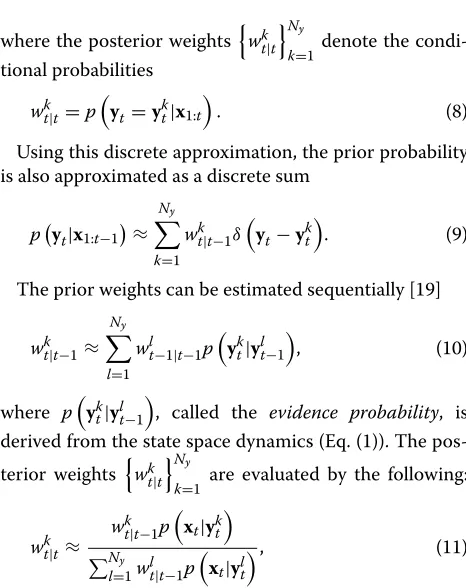
Due to the sequential update of the posterior weights, the converted spectral outputs evolve smoothly in time, within each phonetic segment, also during transitions between phonemes. Figure 1 demonstrates the obtained

0 0.1 0.2 0.3 0.4 0.5 0.6

1 1.5 2 2.5 3 3.5 4

Time [sec]

1st Coefficient

0 0.1 0.2 0.3 0.4 0.5 0.6

−1 −0.5 0 0.5 1 1.5

Time [sec]

3rd Coefficient

Target JGMM GB

time evolution of the first and third Mel frequency cep-strum coefficients (MFCCs) using GB conversion, com-pared to the classical GMM-based conversion—JGMM [2]. The classical GMM-based conversion is applied frame by frame which may lead to discontinuities. The proposed GB, however, is based on a sequential update leading to a smoother time evolution of the cepstral elements, as seen in Fig. 1.

To conclude, the main stages of converting a sequence of source vectors are summarized in Table 2.

4 Discussion

The GB approach uses a state space representation of the source and target spectra to obtain a converted spec-tra as a weighted sum of the target spec-training vectors. In this section, we address two related methods: (1) a method based on state space representation [17] and (2) an exemplar-based approach [18], where the con-verted spectra is evaluated as a weighted sum of the target training vectors. We discuss here the similarities and differences between these methods and our proposed approach.

In [17], a state space approach for representing speech spectra as an observed process generated from an under-ling sequence of a hidden Markov process has been proposed. The source and target speech are both mod-eled using this state space representation. The state space parameters are divided into two parts: a common part related to the uttered speech (assuming a parallel train-ing set) and a differentia part related to the difference between the speakers. These parts are evaluated dur-ing traindur-ing time usdur-ing an iterative algorithm known as expectation maximization (EM) [23]. During the test, the common parameters related to the test utterance are eval-uated using EM and then used, along with the trained differentia part to obtain the converted spectra. Both training and conversion stages include iterative training (EM). Conversion results reported by the authors were obtained using several hundreds of parallel training sen-tences. Although our method and Xu et al.’s method [17] both use state space for representing the temporal evolu-tion of the speech spectra, in our method, the source and

Table 2Voice conversion using GB approximation

Input: a sequence of feature vectors related to the source speakerx1:T

Initialization: set the initial weights,wk 0|0

Ny

k=1.

Main iteration: fort=1,. . .T, perform the following steps:

1. Evaluate the prior weights,wk t|t−1

Ny

k=1, using Eqs. (10) and (16). 2. Evaluate the posterior weights,wk

t|t Ny

k=1, using Eqs. (11) and (14). 3. Evaluatey˜_t=F{xt}, using Eq. (22).

Output: a sequence of converted vectorsy˜_1:T

the target spectra are linked through a state space dynam-ics, while in Xu et al.’s approach, the parallel source and target spectra are each modeled as the observed signals of a shared underlined unobserved Markov process.

An exemplar-based sparse representation approach for voice conversion has been proposed in [18]. Each speech signal is modeled as a linear combination of basis vectors (the training vectors), where the weighting matrix is called an activation matrix. The main assumption used in this method is that the speaker’s identity is modeled by the basis vectors, where the information regarding the uttered text lies entirely in the activation matrix. Therefore, given a test source signal, its activation matrix is evaluated and then multiplied by the target training set, used as the target basis vectors, to obtain the converted spec-tra. Therefore, this method does not require any training, but its testing stage includes high computational load and a substantial memory footprint. As the exemplar-based method, our proposed GB method also uses a linear com-bination of the target training vectors. Besides the obvious differences in the models used by the two methods, there are two major differences: (1) We use sequential evalua-tion of the weights to ensure smooth temporal evoluevalua-tion while in the exemplar-based method, the activation matrix is evaluated as a batch. (2) We use scalar weights while the exemplar-based method uses weighting vectors (the activation matrix).

5 Experimental results 5.1 Experiments setup

In our experiments, we used speech sentences of four US English speakers taken from the CMU ARCTIC database [24]: two males (bdl, rms) and two females (clb, slt). Two different sizes of training sets 5 and 10 parallel sentences were used to demonstrate the performance of the exam-ined methods as a function of training set size. The testing set consisted of 50 additional parallel sentences. All sen-tences were sampled at 16 kHz and were phonetically labeled.

Analysis and synthesis were both carried out using an available vocoder [25]. This vocoder uses a two-band harmonic/noise parametrization, separated by a maximal voicing frequency for representing each spectral envelope [26]. Twenty-five MFCCs were extracted from the har-monic parameters [27]: the zeroth coefficients, related to the energy, were not converted. The other 24 coefficients were used as spectral feature vectors during training and conversion.

parameters by the vocoder. The sequences of the training data set used for GB conversion were matched (without alignment), as described in Section 3.1. The training set used for the other examined methods, and the testing set, were each time aligned using a DTW algorithm based on phonetic labeling [14].

Pitch was converted by a simple linear function using the mean and standard deviation values of the source and target speakers,

ˆ

f₀(y),t=μ(y)+σ(y)/σ(x) f₀(x),t−μ(x), (23)

where f₀(x),t andfˆ₀(y),t are the pitch values of the source and converted signals at thetth frame, respectively. The parametersμ(x) andμ(y)are the mean pitch values, and σ(x) _{and σ}(y) _{are the standard deviations of the source}

and target pitch values, respectively. In this case, the mean and standard deviation of the converted pitch contour match the mean and standard deviation of the pitch values of the target speaker.

5.2 Objective evaluations

We evaluated the performance of the examined con-version methods by two objective measures: normalized distortion (ND) and normalized GV (NGV), as defined below.

To obtain a fair comparison between different source-target pairs, we normalized the mean spectral distor-tion between the converted and target signals by the mean spectral distortion between the source and target signals [30]

ND

˜ Y1:T,Y1:T

=

_T t=1MCD

˜ yt,yt

T

t=1MCD

xt,yt

, (24)

where MCD is the distance between two cepstral vec-tors (defined in Section 3, Eq. (18)) and Y˜1:T

(y˜1,y˜2,. . ., y˜T),Y1:T (y1,y2,. . ., yT), and X1:T

(x1,x2,. . ., xT) are time-aligned sequences of cepstral

vectors, related to the converted, target, and source utter-ances, respectively.

The GV of thepth elements of a sequence,Y˜1:T,

rep-resenting a converted speech utterance, is as follows:

σ2 ˜

Y1:T(p)=

1 T T t=1 ˜ yt(p)−

1 T

T

τ=1 ˜ yτ(p)

2

, (25)

In this paper, we use a normalized global variance (NGV) to measure the variability of a sequence of converted vectors

NGV

˜ Y1:T

1 P P p=1 σ2 ˜

Y_1:T(p)

σ2

Y(p)

, (26)

whereσ_Y2(p)is the empirical GV of thepth elements of the target speaker, obtained from the target training vectors

σ2

Y(p)=

1 Ny

Ny

k=1 ⎛

⎝yk(p)− 1 Ny

Ny

n=1

yn(p)

⎞ ⎠ 2

. (27)

Note that the target GV defined in Eq. (27) is evaluated by averaging over the entire training corpus. This evalu-ation of GV is different from the one proposed in [7] for spectral conversion and GV enhancement, where the GV of each utterance of the target is modeled as a random variable drawn from a Gaussian distribution.

The desired values for these measures are ND → 0 and NGV → 1, indicating that the converted outcome is close to the target signal in terms of spectral similarity and global variance.

The examined GMM-based methods (JGMM and CGMM) were trained using diagonal covariance matri-ces and 1–4 Gaussian mixtures, due to the low amount of training data.

We begin with a short examination of the influence of each of the three parameters of the proposed GB method (Rx, Ry, and τ) on its performance. Figure 2 presents

the ND vs. NGV values obtained for the proposed GB method using Rx ∈ [0.3, 2], Ry ∈ [1, 4], and τ = 1,

trained by 10 sentences, for a male-to-male conversion. As the parameterRx gets higher, more grid points are

con-sidered in the weighted sum, so that ND decreases, but the NGV also decreases. Since the evidence probability is solely determined by the training set (see Eq. (16)), we also examined the performance of the GB method using a data-driven value forRy, specifically, the median of the

MCD between all training vector pairs related to the tar-get speaker. These values vary between 2 and 3 dB when using different source-target pairs and data set sizes. As depicted in Fig. 2, the median leads to the best ND-NGV values so all results presented from now on were obtained using this value forRy.

Figure 3 presents the ND vs. NGV values obtained for the proposed GB method usingRx∈[0.3, 2],τ =(0, 1, 2),

trained by 10 sentences, for a male-to-male conversion. Using τ = 1 leads to higher NGV values than using τ =0, with a slight increase in the ND. However, increas-ingτ further leads to the same NGV values with a minor decrease in the ND.

Table 3 summarizes the ND and NGV values achieved by JGMM [2] and the proposed GB conversion method, for all four gender conversions: male-to-male (M2M),

male-to-female (M2F), female-to-male (F2M), and

female-to-female (F2F), using 5 and 10 training sentences. The number of mixtures for JGMM and parameters for the GB (Rx and τ) were selected for each method and

0.680 0.7 0.72 0.74 0.76 0.78 0.8 0.82 0.84 0.86 0.05

0.1 0.15 0.2 0.25 0.3 0.35 0.4 0.45 0.5

ND

NGV

Ry = 1 Ry = 2dB Ry = Med. Ry = 4dB

Fig. 2ND vs. NGV for GB conversion for a male-to-male conversion using 10 training sentences andRx∈[0.3, 2] dB,τ=1.Ry=1 dB (blue x),

Ry=2 dB (red circle),Ry=median (black asterisk), andRy=3 dB (magenta square)

above, Ry was taken as the median. The proposed GB

leads to higher NGV values in all the cases. For five train-ing sentences, JGMM leads to lower ND values (except for F2M), however, using 10 training sentences, the proposed GB achieves lower or very similar ND values. Still, both methods lead to very low NGV values and consequently, muffled sounding synthesized signals.

To further improve the quality of the synthesized speech, we applied the post-processing method for GV enhancement [21]. This method maximizes the GV of an input sequence, under a spectral distortion constraint. The GV of each enhanced sequence is increased up to the level where the MCD between the converted sequence and its enhanced version reaches a preset threshold value,

0.65 0.7 0.75 0.8 0.85 0.9 0.95 1 1.05 1.1 0

0.05 0.1 0.15 0.2 0.25 0.3 0.35 0.4

ND

NGV

τ

= 0

τ

= 1

τ

= 2

Table 3Objective performance: ND and NGV values using 5 and 10 training sentences, for all four gender conversions

5 Training sentences 10 Training sentences

ND NGV ND NGV

M2M JGMM 0.72 0.15 0.71 0.13

GB 0.73 0.25 0.69 0.14

M2F JGMM 0.7 0.15 0.7 0.12

GB 0.71 0.21 0.69 0.19

F2M JGMM 0.74 0.14 0.71 0.13

GB 0.71 0.34 0.71 0.42

F2F JGMM 0.8 0.22 0.8 0.18

GB 0.88 0.34 0.81 0.31

denoted as θMCD. We recently showed [21] that this method leads to significant improvement in the perceived quality of signals converted by the classical GMM method [1]. In this work, we applied this GV enhancement method to both JGMM and to our proposed GB conversion out-comes. We also examined the performance of CGMM, which considers GV enhancement at training.

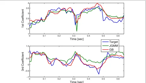
Table 4 summarizes the ND and NGV values achieved by the examined conversion methods, for all four gender conversions using 5 and 10 training sentences.

Again, the GB conversion, followed by GV enhancement withθMCD=2 dB (En-GB) leads to the highest NGV val-ues. Using 5 training sentences, JGMM leads to the lowest ND values, while En-GB comes in second (except for F2F). Using 10 training sentences, En-GB produces the lowest ND and at the same time, the highest NGV, for M2M

Table 4Objective performance: ND and NGV values using 5 and 10 training sentences, for all four gender conversions with GV enhancement (θ=2 dB)

5 Training sentences 10 Training sentences

ND NGV ND NGV

M2M

JGMM 0.76 0.6 0.74 0.55

CGMM 0.83 0.46 0.82 0.45

GB 0.79 0.8 0.73 0.6

M2F JGMM 0.74 0.57 0.74 0.54

CGMM 0.83 0.45 0.84 0.46

GB 0.76 0.73 0.73 0.68

F2M JGMM 0.77 0.63 0.75 0.69

CGMM 0.86 0.62 0.85 0.61

GB 0.76 0.95 0.77 1.1

F2F JGMM 0.86 0.79 0.85 0.65

CGMM 0.91 0.63 0.89 0.6

GB 0.95 1 0.87 0.98

and M2F conversion. For F2M and F2F conversion, En-GB leads to the highest NGV with very similar ND values to JGMM, which are the lowest.

To conclude the objective examination, in terms of NGV, the proposed EN-GB conversion scheme outper-forms all the examined methods. In terms of ND, JGMM leads to lower ND values using 5 training sentences. Using 10 training sentences, En-GB leads to the lowest (or very similar to the lowest) ND values.

In the next section, we present subjective evalua-tion results comparing the proposed En-GB conversion scheme to the classical GMM-based conversion method (with enhancement) and to CGMM, in terms of perceived quality and similarity to the target speaker.

5.3 Subjective evaluations

Listening tests were carried out to subjectively assess the performance of the examined methods (all trained by 10 sentences). In every test, 10 different sentences were examined by 11 listeners (voice samples are available online [31]). The group of listeners included 20–30-year-old, non-experts men and women. The same four speakers (two males and two females) that were used for the objec-tive evaluations were used for the subjecobjec-tive evaluations. The number of mixtures for the GMM-based methods and parameters for the GB conversion (Rx andτ) were

set so minimal spectral distortion would be attained while keeping the NGV as high as possible. We used infor-mal listening tests to select the threshold value for GV enhancement fromθMCD = 0.5, 1, 2, 4 dB. The best per-ceived quality was obtained withθMCD = 2 dB, for both JGMM and GB. All four gender conversions were per-formed using the same parameters values as described above.

CGMM En−GMM En−GB 0

10 20 30 40 50 60 70

Mushra Quality Score

M2M M2F F2M F2F

Fig. 4Subjective quality test, comparing: enhanced JGMM (En-GMM), CGMM [8], and enhanced GB (En-GB)

The listeners were presented with the same test signals (including the hidden reference) and were asked to rate their similarity to the reference signal, in terms of the speaker’s identity, while ignoring their perceived quality. The mean individuality scores of the examined methods for M2M, M2F, F2M, and F2F conversions and also their scores, averaged over all four conversions, are presented in Figs. 6 and 7, respectively.

Except for F2F, the proposed EN-GB was rated as most similar to the target speaker (Fig. 6). In terms of perceived quality, CGMM was rated as having the best quality, while EN-JGMM and EN-GB were rated as comparable (Fig. 4). All in all, considering all four gender conversion, the pro-posed EN-GB was marked as most similar to the target speaker, while CGMM was marked as having the best quality.

CGMM En−GMM En−GB

0 10 20 30 40 50 60

Mushra Quality Score

CGMM En−GMM En−GB 0

10 20 30 40 50 60 70

Mushra Individuality Score

M2M M2F F2M F2F

Fig. 6Subjective individuality test comparing enhanced JGMM (En-GMM), CGMM [8], and enhanced GB (En-GB)

6 Conclusions

Applying voice conversion in low resource environments, such as mobile applications, presents an engineering chal-lenge. While digital processors and memory units become more advanced and less restricting, the amount of avail-able training data remains limited, since most mobile users are not willing to invest much time and effort in recording their own voices. We propose here a GB voice

conversion method suitable for such low resource envi-ronments. It is based on our recent paper, which presents a GB framework for voice conversion. The modified GB method presented in this paper is successfully trained using very few sentences (5–10) and does not require phonetic labeling of the test signals.

The GB conversion method is based on sequential Bayesian tracking, using a GB formulation. The target

CGMM En−GMM En−GB

0 10 20 30 40 50 60

Mushra Individuality Score

spectral evolution is modeled as a hidden Markov pro-cess, tracked by using the source spectrum, modeled as the observed process. The training stage is very simple and based on Euclidean distances between the training vectors, and it is successfully performed using very small training sets. Additionally, although GB is trained using a parallel set, time alignment is not needed. During training, the evidence and likelihood probabilities needed for the GB formulation are approximated as discrete densities. During conversion, the converted spectrum is obtained as a weighted sum of the training target vectors, used as grid points. The weights are sequentially evaluated so that a smooth temporal evolution of the converted spectra is produced.

We used a small set of just 10 sentences for train-ing both the classical GMM-based conversion function and our GB method. According to our experiments, the GB conversion method achieves lower spectral distances between the converted and target spectra and GV val-ues which are closer to the target speaker’s valval-ues than the classical GMM-based conversion. To further improve the quality of the synthesized speech, we increased the variability of the converted vectors by applying GV enhancement as a post-processing block. We compared the proposed En-GB scheme to CGMM and to classical GMM-based conversions, with GV enhancement, using listening tests. This comparison showed that En-GB is the best in terms of similarity to the target speaker and com-parable to the enhanced GMM conversion, in terms of quality.

The proposed GB conversion, as most other methods, simply replaces the spectral envelopes extracted from the source signal with the converted outcome. As a result, the synthesized output has the same speaking rate as the source speaker. Further improvement can be obtained by modifying the duration of each converted utterance to match, on average, its corresponding value for the target speaker.

Spectral distortion and GV are commonly used as objective measures since they provide a simple and fully automated way for evaluating conversion systems. These objective measures may express significant trends and phenomena, but as shown here, they do not always agree with subjective evaluation results.

Further research is needed to design alternative mea-sures for objective evaluation of conversion systems, with better correspondence to subjective results. In the mean time, subjective listening tests are imperative to properly evaluate and compare conversion methods.

The proposed GB conversion method, as presented here, is based on soft correspondence between the source and target vectors, obtained by using a parallel training set. Further research is needed to evaluate this correspon-dence for a non-parallel setup.

Endnotes

1_{In general, any arbitrary integrable function of the}

state vectory_tcan be evaluated [19].

2_{If the state space is indeed discrete and finite, and the}

grid points consist of all its states, this evaluation becomes exact.

Competing interests

The authors declare they have no competing interests.

Authors’ contributions

This paper is part of the doctoral research work of HB under the supervision of the other two authors.

Acknowledgements

The authors would like to thank Slava Shechtman, and the speech research group headed by Ron Hoory, at the IBM Research Labs, Haifa, Israel, for fruitful discussions.

Received: 20 March 2015 Accepted: 7 January 2016

References

1. OYC Stylianou, E Moulines, Continuous probabilistic transform for voice conversion. IEEE Trans. Speech Audio Proc.6(2), 131–142 (1998) 2. A Kain, M Macon, inProc. ICASSP. Spectral voice conversion for

text-to-speech synthesis (IEEE, Seattle, Washington, USA, 1998), pp. 285–288

3. T Toda, AW Black, K Tokuda, inProc. ICASSP. Spectral conversion based on maximum likelihood estimation considering global variance of converted parameter (IEEE, Philadelphia, Pennsylvania, USA, 2005), pp. 9–12 4. T Toda, H Saruwatari, K Shikano, inProc. ICASSP. Voice conversion

algorithm based on Gaussian mixture model with dynamic frequency warping of STRAIGHT spectrum (IEEE, Orlando, Florida, USA, 2001), pp. 841–844

5. A Kain, MW Macon, inProc. ICASSP. Design and evaluation of a voice conversion algorithm based on spectral envelope mapping and residual prediction (IEEE, Salt Lake City, Utah, USA, 2001), pp. 813–816

6. T En-Najjary, O Rosec, T Chonavel, inProc. Interspeech ICSLP. A voice conversion method based on joint pitch and spectral envelope transformation, (Jeju Island, Korea, 2004), pp. 1225–1225 7. T Toda, AW Black, K Tokuda, Voice conversion based on

maximum-likelihood estimation of spectral parameter trajectory. IEEE Trans. Audio Speech Lang. Proc.15(8), 2222–2235 (2007)

8. H Benisty, D Malah, inProc. Interspeech. Voice conversion using GMM with enhanced global variance (ISCA, Florence, Italy, 2011), pp. 669–672 9. T Toda, T Muramatsu, H Banno, inINTERSPEECH. Implementation of computationally efficient real-time voice conversion (ISCA, Portland, Oregon, U.S, 2012). Citeseer

10. T Muramatsu, Y Ohtani, T Toda, H Saruwatari, K Shikano, inInterspeech. Low-delay voice conversion based on maximum likelihood estimation of spectral parameter trajectory (ISCA, 2008), pp. 1076–1079

11. Y Nankaku, K Nakamura, T Toda, K Tokuda, inProc. Interspeech. Spectral conversion based on statistical models including time-sequence matching (ISCA, 2007), pp. 333–338

12. D Erro, A Moreno, A Bonafonte, Inca algorithm for training voice conversion systems from nonparallel corpora. Audio Speech Lang. Process. IEEE Trans.18(5), 944–953 (2010)

13. H Benisty, D Malah, K Crammer, inProc. ICASSP. Non-parallel voice conversion using joint optimization of alignment by temporal context and spectral distortion (IEEE, Florence, Italy, 2014), pp. 7909–7913 14. D Erro, A Moreno, A Bonafonte, Voice conversion based on weighted

frequency warping. IEEE Trans. Audio Speech Lang. Proc.18(5), 922–931 (2010)

15. E Helander, J Schwarz, SHJ Nurminen, M Gabbouj, inProc. Interspeech. On the impact of alignment on voice conversion performance (ISCA, Brisbane, Australia, 2008), pp. 1453–1456

17. N Xu, Z Yang, L Zhang, W Zhu, J Bao, Voice conversion based on state-space model for modelling spectral trajectory. Electron. Lett.45(14), 763–764 (2009)

18. Z Wu, T Virtanen, ES Chng, H Li, Exemplar-based sparse representation with residual compensation for voice conversion. Audio Speech Lang. Process. IEEE/ACM Trans.22(10), 1506–1521 (2014)

19. MS Arulampalam, S Maskell, N Gordon, T Clapp, A tutorial on particle filters for online nonlinear/non-Gaussian Bayesian tracking. IEEE Trans. Signal Proc.50(2), 174–188 (2002)

20. H Benisty, D Malah, K Crammer, inElectrical & Electronics Engineers in Israel (IEEEI), 2014 IEEE 28th Convention Of. Sequential voice conversion using grid-based approximation (IEEE, 2014), pp. 1–5

21. H Benisty, D Malah, K Crammer, inProc. EUSIPCO. Modular global variance enhancement for voice conversion systems, (2012), pp. 370–374 22. B Anderson, J Moore,Optimal Filtering. (Prentice-Hall, Englewood Cliffs,

NJ, 1979)

23. A Dempster, N Laird, D Rubin, Maximum likelihood from incomplete data via the EM algorithm. J. R. Stat. Soc. B.39, 1–38 (1977)

24. J Kominek, AW Black,CMU ARCTIC Databases for Speech Synthesis, (2003) 25. Aholab Coder. http://aholab.ehu.es/ahocoder/. Accessed Jan 2013 26. D Erro, I Sainz, I Hernaez, inProc. Interspeech. Improved HNM-based

vocoder for statistical synthesizers, (2011), pp. 1809–1812

27. O Cappe, E Moulines, Regularization techniques for discrete cepstrum estimation. IEEE Signal Process. Lett.3(4), 100–102 (1996)

28. H Kuwabara, Y Sagisaka, Acoustic characteristics of speaker individuality: control and conversion. IEEE Trans. Signal Proc.16(2), 165–173 (1995) 29. D Erro, A Moreno, A Bonafonte, Inca algorithm for training voice

conversion systems from nonparallel corpora. IEEE Trans. Audio Speech Lang. Proc.18(5), 944–953 (2010)

30. H Ye, S Young, Quality-enhanced voice morphing using maximum likelihood transformations. IEEE Trans. Audio Apeech Lang. Proc.14(4), 1301–1312 (2006)

31. Sound Samples. http://sipl.technion.ac.il/Info/hadas/sound-samples.htm Accessed Mar 2015

32. Multi stimulus test with hidden reference and anchors (MUSHRA) (2003). Technical Report ITU-R BS.1534-1, International Telecommunications Union

33. E Godoy, O Rosec, T Chonavel, Voice conversion using dynamic frequency warping with amplitude scaling, for parallel or nonparallel corpora. IEEE Trans. Audio Speech Lang. Proc.20(4), 1313–1323 (2012)

Submit your manuscript to a

journal and benefi t from:

7Convenient online submission 7Rigorous peer review

7Immediate publication on acceptance 7Open access: articles freely available online 7High visibility within the fi eld

7Retaining the copyright to your article