The Thirty-Third AAAI Conference on Artificial Intelligence (AAAI-19)
Pareto Optimization for Subset Selection with Dynamic Cost Constraints
Vahid Roostapour,
1Aneta Neumann,
1Frank Neumann,
1Tobias Friedrich
1, 21Optimisation and Logistics, School of Computer Science, The University of Adelaide, Adelaide, Australia 2Chair of Algorithm Engineering, Hasso Plattner Institute, Potsdam, Germany
{vahid.roostapour, aneta.neumann, frank.neumann}@adelaide.edu.au, [email protected]
Abstract
In this paper, we consider the subset selection problem for functionfwith constraint boundBwhich changes over time. We point out that adaptive variants of greedy approaches commonly used in the area of submodular optimization are not able to maintain their approximation quality. Investigat-ing the recently introduced POMC Pareto optimization ap-proach, we show that this algorithm efficiently computes a
φ= (αf/2)(1− 1
eαf)-approximation, whereαf is the
sub-modularity ratio of f, for each possible constraint bound
b ≤ B. Furthermore, we show that POMC is able to adapt its set of solutions quickly in the case thatBincreases. Our experimental investigations for the influence maximization in social networks show the advantage of POMC over general-ized greedy algorithms.
Introduction
Many combinatorial optimization problems consist of opti-mizing a given function under a given constraint. Constraints often limit the resources available to solve a given problem and may change over time. For example, in the area of sup-ply chain management, the problem may be constrained by the number of vehicles available which may change due to vehicle failures and vehicles being repaired or added as a new resource.
Submodular functions form an important class of prob-lems as many important optimization probprob-lems can be mod-eled by them. The area of submodular function optimiza-tion under given static constraints has been studied quite ex-tensively in the literature (Nemhauser, Wolsey, and Fisher 1978; Lee et al. 2010; Lee, Sviridenko, and Vondr´ak 2010; Krause and Golovin 2014). In the case of monotone sub-modular functions, greedy algorithms are often able to achieve the best possible worst case approximation guaran-tee (unless P=NP).
Recently, Pareto optimization approaches have been in-vestigated for a wide range of subset selection prob-lems (Friedrich and Neumann 2015; Qian, Yu, and Zhou 2015; Qian et al. 2017a; 2017b). It has been shown in (Qian et al. 2017b) that an algorithm called POMC is able to achieve aφ = (αf/2)(1−eαf1 )-approximation whereαf
Copyright c2019, Association for the Advancement of Artificial Intelligence (www.aaai.org). All rights reserved.
measures the closeness of the considered functionf to sub-modularity. The approximation matches the worst-case per-formance ratio of the generalized greedy algorithm (Zhang and Vorobeychik 2016).
Our contribution
In this paper, we study monotone functions with a con-straint where the concon-straint bound B changes over time. Such constraint changes reflect real-world scenarios where resources vary during the process. We show that greedy al-gorithms have difficulties in adapting their current solutions after changes have happened. In particular, we show that there are simple dynamic versions of the classical knap-sack problem where adding elements in a greedy fashion when the constraint bound increases over time can lead to an arbitrary bad performance ratio. For the case where con-straint bounds decrease over time, we introduce a submod-ular graph covering problem and show that the considered adaptive generalized greedy algorithm may encounter an ar-bitrarily bad performance ratio on this problem.
Investigating POMC, we show that this algorithm obtains for each constraint bound b ∈ [0, B], a φ = (αf/2)(1−
1
eαf)-approximation efficiently. Furthermore, when relaxing
the boundB toB∗ > B,φ-approximations for all values ofb∈[0, B∗]are obtained efficiently. We evaluate the con-sidered algorithms on influence maximization in social net-works that have dynamic routing or cardinality constraints. Benchmarking the algorithms over sequences of dynamic changes, we show that POMC obtains superior results to the generalized greedy and adaptive generalized greedy algo-rithms. Furthermore, POMC shows an even more prominent advantage as more dynamic changes are carried out because it is able to improve the quality of its solutions and cater for changes that occur in the future.
Problem Formulation and Algorithms
In this paper we consider optimization problems in which the cost function and objective functions are monotone and quantified according to their closeness to submodularity.
Different definitions are given for submodularity (Nemhauser, Wolsey, and Fisher 1978) and we use the fol-lowing one in this paper. For a given setV ={v1,· · · , vn},
a functionf : 2V →Ris submodular if for anyX ⊆Y ⊆V andv /∈Y
f(X∪v)−f(X)≥f(Y ∪v)−f(Y). (1)
In addition, we consider how much a function is close to being submodular, measured by the submodularity ra-tio (Zhang and Vorobeychik 2016). The funcra-tion f isαf
-submodular where
αf = min
X⊆Y,v /∈Y
f(X∪v)−f(X)
f(Y ∪v)−f(Y).
This definition is equivalent to the Equation 1 whenαf = 1,
i.e. we have submodularity in this case. Another notion which is used in our analysis is the curvature of function f. The curvature measures the deviation from linearity and reflects the effect of marginal contribution according to the functionf (Conforti and Cornu´ejols 1984; Vondr´ak 2010). For a monotone submodular functionf : 2V →R+,
κf = 1−min
v∈V
f(V)−f(V \v)
f(v)
is defined as the total curvature off.
In many applications the function to be optimized f comes with a cost functioncwhich is subject to a given cost constraintB. Often the cost functionccannot be evaluated precisely. Hence, the functionˆc which isψ-approximation ofcis used (Zhang and Vorobeychik 2016). Moreover, ac-cording to the submodularity off, the aim is to find a good approximation instead of finding the optimal solution.
Consider the static version of an optimization problem de-fined in (Qian et al. 2017b).
Definition 1(The Static Problem). Given a monotone ob-jective function f : 2V →
R+, a monotone cost function
c : 2V → R+ and a budgetB, the goal is to compute a
solutionXsuch that
X= arg max
Y⊆V
f(Y)s.t.c(Y)≤B.
As for the static case investigated in (Qian et al. 2017b), we are interested in aφ-approximation whereφ= (αf/2)(1−eαf1 )depends on the submodularity ratio.
Zhang and Vorobeychik considered the performance of the generalized greedy algorithm (Zhang and Vorobeychik 2016), given in Algorithm 1, according to the approximated cost functionˆc. Starting from the empty set, the algorithm always adds the element with the largest objective to cost ratio that does not violate the given constraint boundB.
Let Kc = max{|X| : c(X) ≤ B}. The optimal
so-lution X˜B in these investigations is defined as X˜B =
arg max{f(X)|c(X)≤αc
B(1+α2
c(Kc−1)(1−κc)))
ψKc }where
αc is the submodularity ratio of c. This formulation gives
the value of an optimal solution for a slightly smaller bud-get constraint. The goal is to obtain a good approximation of f( ˜XB)in this case.
It has been shown in (Zhang and Vorobeychik 2016) that the generalized greedy algorithm, which adds the item with the highest marginal contribution to the current solution in each step, achieves a(1/2)(1−1
e)-approximate solution iff
is monotone and submodular. (Qian et al. 2017b) extended these results to objective functions withαf submodularity
ratio and proved that the generalized greedy algorithm ob-tains aφ= (αf/2)(1−eαf1 )-approximation. For the
remain-der of this paper, we assumeφ= (αf/2)(1−eαf1 )and are
interested in obtaining solutions that are φ-approximation for the considered problems.
In this paper, we study the dynamic version of problem given in Definition 1.
Definition 2 (The Dynamic Problem). Let X be a φ -approximation for the problem in Definition 1. The dynamic problem is given by a sequence of changes where in each change the current budget B changes to B∗ = B +d,
d ∈R≥−B. The goal is to compute aφ-approximationX0
for each newly given budgetB∗.
The Dynamic Problem evolves over time by the changing budget constraint bounds. Note that every fixed constraint bound gives a static problem and any good approximation algorithm can be run from scratch for the newly given bud-get. However, the main focus of this paper are algorithms that can adapt to changes of the constraint bound.
Algorithms
We consider dynamic problems according to Definition 2 withφ= (αf/2)(1−eαf1 )and are interested in algorithms
that adapt their solutions to the new constraint bound B∗ and obtain aφ-approximation for the new boundB∗. As the generalized greedy algorithm can be applied to any bound B, the first approach would be to run it for the newly given boundB∗. However, this might lead to totally different so-lutions and adaptation of already obtained soso-lutions might be more beneficial. Furthermore, adaptive approaches that change the solution based on the constraint changes are of interest as they might be faster in obtaining such solutions and/or be able to learn good solutions for the different con-straint bounds that occur over time.
Based on the generalized greedy algorithm, we introduce the adaptive generalized greedy algorithm. This algorithm is modified from Algorithm 1 in a way that enables it to deal with a dynamic change. Let X be the current solution of the algorithm. When a dynamic change decreases the bud-get constraint, the algorithm removes items fromX accord-ing to their marginal contribution, until it achieves a feasible solution. When there is a dynamic increase, this algorithm behaves similarly to the generalized greedy algorithm.
Algorithm 1:Generalized Greedy Algorithm
input:Initial budget constraintB.
1 X ← ∅;
2 V0←V;
3 repeat
4 v∗←arg maxv∈V0 fˆc((XX∪∪vv))−−cfˆ((XX));
5 ifˆc(X∪v∗)≤Bthen
6 X ←X∪v∗;
7 V0←V0\ {v∗};
8 untilV0← ∅;
9 v∗←arg maxv∈V;ˆc(v)≤Bf(v); 10 returnarg maxS∈{X,v∗}f(S);
Algorithm 2:Adaptive Generalized Greedy Algorithm
input:Initial solutionX, Budget constraintB, New budget constraintB∗.
1 ifB∗< Bthen
2 whileˆc(X)> B∗do
3 v∗←arg minv∈Xf(X)−f(X\{v}) ˆ
c(X)−ˆc(X\{v});
4 X ←X\ {v∗};
5 else ifB∗> Bthen
6 V0←V \X;
7 repeat
8 v∗←arg maxv∈V0 fˆc((XX∪∪vv))−−cfˆ((XX));
9 ifˆc(X∪v∗)≤B∗then
10 X ←X∪v∗;
11 V0←V0\ {v∗};
12 untilV0← ∅;
13 v∗←arg maxv∈V;ˆc(v)≤B∗f(v); 14 returnarg maxS∈{X,v∗}f(S);
optimization approach which is proven to perform better than the generalized greedy algorithm in case of local op-tima (Qian et al. 2017b). We reformulate the problem as a bi-objective problem in order to use POMC as follows:
arg maxX ∈ {0,1}n(f1(X), f2(X)),
where:
f1(X) =
−∞, cˆ(X)> B+ 1
f(X), otherwise , f2(X) =−cˆ(X).
This algorithm optimizes the cost function and the ob-jective function simultaneously. To achieve this, it uses the concept of dominance to compare two solutions. Solution X1 dominates X2, denoted by X1 X2, if f1(X1) ≥ f1(X2)∧f2(X1) ≥ f2(X2). The dominance is strict,,
when at least one of the inequalities is strict. POMC pro-duces a population of non-dominated solutions and opti-mizes them during the optimization process. In each itera-tion, it chooses solutionX randomly from the population and flips each bit of the solution with the probability of1/n. It adds the mutated solution X0 to the population only if
Algorithm 3:POMC Algorithm
input:Initial budget constraintB, timeT
1 X ← {0}n;
2 Compute(f1(X), f2(X));
3 P ← {x};
4 t←0;
5 whilet < T do
6 SelectX fromPuniformly at random;
7 X0←flip each bit ofX with probabilityn1; 8 Compute(f1(X0), f2(X0));
9 if@Z ∈Psuch thatZ X0then
10 P ←(P\ {Z ∈P |X0 Z})∪ {X0};
11 t=t+ 1;
12 returnarg maxX∈P:ˆc(X)≤Bf(x)
there is no solution in the population that dominates X0. All the solutions which are dominated byX0will be deleted from the population afterward.
Note that we only compute the objective vector
(f1(X), f2(X))when the solution X is created. This
im-plies that the objective vector is not updated after changes to the constraint boundB. As a consequence solutions whose constraint exceeds the value of B + 1 for a newly given bound are kept in the population. However, newly produced individuals exceeding B + 1for the current bound B are not included in the population as they are dominated by the initial search point 0n. We are using the valueB + 1
in-stead ofBin the definition off1as this gives the algorithm
some look ahead for larger constraint bounds. However, ev-ery value of at leastBwould work for our theoretical anal-yses. The only drawback would be a potentially larger pop-ulation size which influences the valuePmaxin our runtime
bounds.
Adaptive Generalized Greedy Algorithm
In this section we analyze the performance of the adaptive generalized greedy algorithm. This algorithm is a modified version of the generalized greedy using the same principle in adding and deleting items. However, in this section we prove that the adaptive generalized greedy algorithm is not able to deal with the dynamic change, i.e., the approximation obtained can become arbitrarily bad during a sequence of dynamic changes.
In order to show that the adaptive generalized greedy al-gorithm can not deal with dynamic increases of the con-straint bound, we consider a special instance of the classical knapsack problem. Note that the knapsack problem is spe-cial submodular problem where both the objective and the cost function are linear.
Givenn+ 1itemsei = (ci, fi)with costci and value
fiindependent of the choice of the other items, we assume
there are items ei = (1,n1), 1 ≤ i ≤ n/2,ei = (2,1),
n/2 + 1 ≤ i ≤ n, and a special itemen+1 = (1,3). We
havefinc(X) =Pei∈Xfiandcinc(X) =
P
ei∈Xcias the
⋯
⋯
"
#$"
%$&
#$&
%$&
*$&
)$&
%' (*$&
%'(%$"
'$"
*$⋯
⋯
Figure 1: Single subgraphGiofG= (U, V, E)
Theorem 3. Given the dynamic knapsack problem (finc, cinc), starting withB = 1and increasing the bound
n/2 times by1, the adaptive generalized greedy algorithm computes a solution that has approximation ratioO(1/n).
Proof. For the constraint B = 1 the optimal solution is {en+1}. Now let there ben/2dynamic changes where each
of them increases B by 1. In each change, the algorithm can only pick an item from{e1,· · ·, en/2}, otherwise it
vi-olates the budget constraint. After n/2 changes, the bud-get constraint is1 +n/2and the result of the algorithm is S={en+1, e1,· · ·, en/2}withf(S) = 3+(n/2)·(1/n) =
7/2 and c(S) = 1 +n/2. However, an optimal solution for budget1 +n/2isS∗ ={en+1, en/2+1, . . . , e3n
4 }with
f(S∗) = 3 +n4. Hence, the approximation ratio in this ex-ample is(7/2)/(3 +n/4) =O(1/n)
Now we consider the case where the constraint bound de-creases over time and show that the adaptive generalized greedy algorithm may also encounter situations where the approximation ratio becomes arbitrarily bad over time.
We consider the followingGraph Coverage Problem. Let G = (U, V, E)be a bipartite graph with bipartitionU and V of vertices with|U| = nand|V| = m. The goal is to select a subsetS ⊆U with|S| ≤Bsuch that the number of neighbors ofS inV is maximized. Note that the objective functionf(S)measuring the number of neighbors ofSinV is monotone and submodular.
We consider the graphG= (U, V, E)which consists ofk disjoint subgraphs
Gi= (Ui={ui1,· · · , u
i
l}, Vi={v1i,· · · , v
i
2l−2}, Ei)
(see Figure 1). Nodeui
1 is connected to nodesvi2j−1,1 ≤ j≤l−1. Moreover, each vertexui
j,2≤j≤lis connected
to two verticesvi
2j−3andvi2j−2. We assume thatk =
√
n andl=n/k=√n.
Theorem 4. Starting with the optimal setS =U and bud-getB =n, there is a specific sequence of dynamic budget reductions such that the solution obtained by the adaptive generalized greedy algorithm has the approximation ratio
O(1/√n).
Proof. Let the adaptive generalized greedy algorithm be ini-tialized withX =U andB =n=kl. We assume that the budget decreases from nto k where each single decrease reduces the budget by1. In the firstksteps, to change the
cost of solution fromnton−k, the algorithm removes the nodesui
1,1 ≤i ≤k, as they have a marginal contribution
of0. Following these steps, all the remaining nodes have the same marginal contribution of 2. The solutionX of sizek obtained by the removal steps of the adaptive generalized greedy algorithm containskvertices which are connected to
2knodes ofV, thusf(X) = 2k = 2√n. Such a solution is returned by the algorithm forB=kas the most valuable single node has at most(l−1) = (√n−1)neighbors inV. ForB=k, the optimal solutionX∗={ui1|1≤i≤k}has f(X∗) =k(l−1) =n−√n. Therefore, the approximation ratio achieved by the adaptive generalized greedy algorithm is upper bounded by(2√n)/(n−√n) =O(1/√n).
Pareto Optimization
In this section we analyze the behavior of POMC fac-ing a dynamic change. Accordfac-ing to Lemma 3 in (Qian et al. 2017b), we have for any X ⊆ V and v∗ = arg maxv /∈X fcˆ((XX∪∪vv))−−cfˆ((XX)):
f(X∪v∗)−f(X)≥αf
ˆ
c(X∪v∗)−ˆc(X)
B ·(f( ˜X)−f(X)). We denote byδˆc= min{ˆc(X∪v)−cˆ(X)|X ⊆V, v /∈
X}the smallest contribution of an element to the cost of a solution for the given problem. Moreover, letPmaxbe the
maximum size of POMC’s population during the optimiza-tion process.
The following theorem considers the static case and shows that POMC computes a φ-approximation efficiently for every budgetb∈[0, B].
Theorem 5. Starting from{0}n, POMC computes, for any
budgetb ∈[0, B], aφ = (αf/2)(1−1/eαf)-approximate
solution afterT =cnPmax·δBˆc iterations with the constant
probability, wherec≥8e+ 1is a sufficiently large arbitrary constant.
Proof. We first consider the number of iterations to find a
(αf/2) 1−(1−
αf
k )
k
-approximate solution for a budget b ∈ [0, B] and some k. We consider the largest value of i for which there is a solutionX in the population where
ˆ
c(X)≤i < band
f(X)≥ 1−
1−αf
i bk
k! ·f( ˜Xb)
holds for somek. Initially, it is true fori = 0 withX =
{0}n. We now show that addingv∗ to the current solution
has the desired contribution to achieve aφ-approximate so-lution. LetX ⊆V andv∗= arg maxv /∈X fcˆ((XX∪∪vv))−−cfˆ((XX)).
Assume that
f(X)≥ 1−
1−αf
i bk
k! ·f( ˜Xb)
holds for someˆc(X)≤i < bandk. Then addingv∗leads to
f(X∪v∗)≥
1−
1−αf
i+ ˆc(X∪v∗)−ˆc(X)
b(k+ 1)
k+1!
This process only depends on the quality ofX and is inde-pendent from its structure. Starting from{0}n, if the
algo-rithm carries out such steps at leastb/δˆc times, it reaches a
solutionXsuch that
f(X∪v∗)≥ 1−
1−αf
b bk∗
k∗! ·f( ˜Xb)
≥
1− 1
eαf
·f( ˜Xb).
Considering itemz= arg maxv∈V:ˆc(v)≤bf(v), by
submod-ularity and α ∈ [0,1] we have f(X ∪v∗) ≤ (f(X) +
f(z))/αf.
This implies that
max{f(X), f(z)} ≥(αf/2)·(1−
1
eαf)·f( ˜Xb).
We considerT =cnPmaxB/δˆciterations of the algorithm
and analyze the success probability withinTsteps. To have a successful mutation step wherev∗is added to the currently best approximate solution, the algorithm has to choose the right individual in the population, which happens with prob-ability at least 1/Pmax. Furthermore, the single bit
corre-sponding tov∗ has to be flipped which has the probability at least1/(en). We call such a step a success. Let random variableYj = 1when there is a success in iterationjof the
algorithm andYj= 0, otherwise. Thus, we have
Pr(Yj = 1)≥
1
en ·
1
Pmax
as long as aφ-approximation for boundbhas not been ob-tained.
Furthermore, letYi∗,1≤i≤T, be mutually independent random binary variables withPr[Yi∗ = 1] = enP1
max and
Pr[Yi∗ = 0] = 1− 1
enPmax. For the expected value of the random variableY∗=PT
j=1Yj∗we have:
E[Y∗] = T
enPmax
= cB
eδˆc
≥ cb
eδˆc
.
We use Lemma 1 in (Doerr, Happ, and Klein 2011) for mod-erately correlated variables which allows the use of the fol-lowing Chernoff bound
Pr (Y <(1−δ)E[Y∗])≤Pr (Y∗<(1−δ)E[Y∗])
≤e−E[Y∗]δ2/2. (2)
Using Equation 2 with δ = (1 − e
c), we bound the
probability of not finding aφ-approximation ofX˜b in time
T =cnPmaxB/δˆcby
Pr(Y ≤ b
δˆc
)≤e−
(c−e)2B
2ceδˆc ≤e−
(c/2)2B
2ceδˆc
≤e−8cBeδˆc ≤e− B δˆc.
Using the union bound and taking into account that there are at mostB/δˆcdifferent values forbto consider, the
proba-bility that there is ab∈[0, B]for which noφ-approximation
has been obtained is upper bounded by δB ˆ
c ·e
−B δˆc.
This implies that POMC finds a (αf/2)(1 − eαf1 )
-approximate solution with probability at least1−B δˆc·e
−B δˆc
for eachb∈[0, B].
Note that if we haveB/δˆc ≥ lognthen the probability
of achieving aφ-approximation for everyb∈ [0, B]is1−
o(1). In order to achieve a probability of1−o(1)for any possible change, we can run the algorithm forT0=cnPmax·
max{logn,Bδ
ˆ
c},c≥8e+ 1, iterations.
Now we consider the performance of POMC in the dy-namic version of the problem. In this version, it is assumed that POMC has achieved a population which includes aφ -approximation for all budgetsb∈[0, B]. Reducing the bud-get from B toB∗ implies that a φ-approximation for the newly given budgetB∗ is already contained in the popula-tion.
Consideration must be given to the case where the bud-get increases. Assume that the budbud-get changes from B to B∗ = B +d where d > 0. We analyze the time until POMC has updated its population such that it contains for anyb∈[0, B∗]aφ-approximate solution.
We define
Imax(b, b0) = max{i∈[0, b]| ∃X ∈P,ˆc(X)≤i
∧f(X)≥ 1−
1−αf
i bk
k! ·f( ˜Xb)
∧f(X)≥ 1−
1−αf
i b0k0
k0!
·f( ˜Xb0)}
for somekandk0. The notion of Imax(b, b0)enables us to
correlate progress in terms of obtaining aφ-approximation for budgetsbandb0.
Theorem 6. Let POMC have a population P such that, for every budget b ∈ [0, B], there is a φ-approximation inP. After changing the budget to B∗ > B, POMC has computed a φ-approximation with probabilityΩ(1) within
T =cnPmaxδd
ˆ
c steps for everyb∈[0, B
∗].
Proof. Let P denote the current population of POMC in which, for any budgetb ≤ B, there is a 1−(1−αf
k )
k
-approximate solution for somek.
LetXbe the solution corresponding toImax(B, B∗). Let v∗ = arg maxv /∈X fcˆ((XX∪∪vv))−−ˆfc((XX)) be the item with the high-est marginal contribution which could be added toX and X0 = X ∪v∗. According to Lemma 3 and Theorem 2 in (Qian et al. 2017b) and the definition ofImax(B, B∗), we
have
f(X0)≥
1−(1−αf
Imax+ ˆc(X0)−ˆc(X)
Bk )
k
·f( ˜XB)
and
f(X0)≥
1−(1−αf
Imax+ ˆc(X0)−ˆc(X)
B∗k0 )
k0
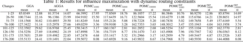
Table 1: Results for influence maximization with dynamic routing constraints
Changes GGA AGGA POMC1000 POMC5000 POMC10000 POMCWP1000 POMCWP5000 POMCWP10000
mean st mean st mean st mean st mean st mean st mean st mean st 1-25 85.0349 12.88 81.5734 14.07 66.3992 17.95 77.8569 18.76 86.1057 17.22 86.3846 10.76 86.9270 12.86 85.8794 14.69 26-50 100.7344 22.16 96.1386 23.99 104.9102 15.50 117.6439 16.71 122.5604 15.54 110.4279 11.08 115.6766 14.21 120.8651 14.97 51-75 118.1568 30.82 110.4893 29.50 141.8249 5.64 155.2126 5.08 158.7228 5.20 140.7838 5.02 149.7658 5.49 157.6169 5.54 76-100 127.3422 31.14 115.2978 27.66 149.0259 3.36 159.9100 3.28 162.7353 3.65 148.3012 3.47 155.1943 4.04 163.1958 3.74 101-125 132.3502 29.62 116.9768 25.45 150.3415 3.17 160.1367 2.81 161.2852 2.68 148.5254 2.67 155.1104 3.05 162.3770 2.81 126-150 134.5256 27.69 118.6962 24.19 147.8998 7.36 154.7319 8.77 154.1470 7.43 143.4908 7.96 150.7567 7.82 156.0363 8.12 151-175 135.7651 25.89 119.4982 22.85 147.2478 4.68 153.1417 5.32 151.2966 3.17 143.2959 4.79 149.5447 4.87 153.2526 3.85 176-200 135.5133 24.41 119.1491 22.04 139.5072 8.08 143.6928 9.16 143.9832 8.67 134.7968 8.72 140.5930 8.61 144.4088 8.08
This implies that adding v∗ toX violates the budget con-straintB, otherwise we would have a greater value forImax.
IfImax+ ˆc(X0)−ˆc(X)≥B∗, then, similar to the proof
of Theorem 5, we have
max{f(X), f(z)} ≥(αf/2)·
1− 1
eαf
·f( ˜XB∗).
Otherwise, we have
f(X0)≥
1−(1−αf
B B∗k0)
k0
·f( ˜XB∗).
From this point, the argument in the proof of Theorem 5 holds, i.e., POMC obtains, for each value b ∈ [B, B∗], a φ-approximation after δd
ˆ
c successes.
Hence, after T = cnPmaxd/δˆc iterations, for all b ∈
[B, B∗] with probability 1 − d
δˆc ·e
−d
δˆc, we have a φ =
(αf/2)(1−eαf1 )-approximation in the population.
Note that if the dynamic change is sufficiently large such that δd
ˆ
c ≥logn, then the probability of having obtained, for
every budgetb ∈ [0, B∗], a φ-approximation increases to 1−o(1). A success probability of1−o(1)can be obtained for this magnitude of changes by giving the algorithm time T0=cnPmaxmax{logn,δd
ˆ
c},c≥8e+ 1.
A special class of known submodular problems is the maximization of a function with a cardinality constraint. In this case, the constraint value can take on at mostn+ 1 dif-ferent values and we havePmax ≤n+ 1. Furthermore, we
haveδ= 1which leads to the following two corollaries.
Corollary 7. Consider the static problem with cardinality constraint boundB. POMC computes, for every budgetb∈
[0, B], aφ-approximation withinT =cn2·max{B,logn}, c≥8e+ 1, iterations with probability1−o(1).
Corollary 8. Consider the dynamic problem with a car-dinality constraint B. Assume that P contains a φ -approximation for every b ∈ [0, B]. Then after increasing the budget toB∗, POMC computes, for every budget b ∈
[0, B∗], aφ-approximation in timeT =cn2max{d,logn}, c≥8e+ 1andd=|B∗−B|, with probability1−o(1).
Experimental Investigations
We compare the generalized greedy algorithm (GGA) and adaptive generalized greedy algorithm (AGGA) with the POMC algorithm on the submodular influence maximiza-tion problem (Zhang and Vorobeychik 2016; Qian et al. 2017b). We consider dynamic variants of the problems where the constraint bound changes over time.
The Influence Maximization Problem
The influence maximization problem aims to identify a set of most influential users in a social network. Given a directed graph G = (V, E) where each node repre-sents a user. Each edge (u, v) ∈ E has assigned an edge probability pu,v((u, v) ∈ E). The probability pu,v
corresponds to the strengths of influence from user u to user v. The goal is to find a subset X ⊆ V such that the expected number of activated nodes from X, IC(X), is maximized. Given a cost function c and a budget B the submodular optimization problem is formulated as
arg maxX⊆VE[|IC(X)|]s.t.c(X)≤B.
We consider two types of cost functions. The routing constraint takes into account the costs of visiting nodes whereas the cardinality constraint counts the number of cho-sen nodes. For both cost functions, the constraint is met if the cost is at mostB.
For more detailed descriptions of the influence maximiza-tion through a social network problem we refer the reader to (Kempe, Kleinberg, and Tardos 2015; Zhang and Vorobey-chik 2016; Qian et al. 2017b).
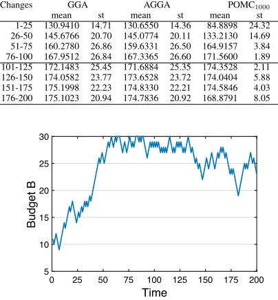
For our dynamic constraint bound changes, we follow the approach taken in (Roostapour, Neumann, and Neumann 2018). We assume that the initial constraint bound isB= 10
and stays within the interval[5,30]. We consider a sequence of 200constraint bounds obtained by randomly increasing or decreasing B by a value of 1. The values of B over time used in our studies are shown in Figure 2. For the ex-perimental investigations of POMC, we consider a parame-terτwhich determines the number of generations between constraint changes. Furthermore, we consider the option of POMC having a warm-up phase where there are no dynamic changes for the first 10000 iterations. This allows POMC to optimize for an extended period for the initial bound. It should be noted that the number of iterations in the warm-up phase and our choices ofτare relatively small compared to the choice of10eBn2used in (Qian et al. 2017b) for
op-timizing the static problem with a given fixed boundB. The results are shown in Tables 1 and 2 and we report for each batch of25consecutive constraint bound changes the aver-age solution quality and standard deviation.
Influence Maximization with Dynamic Routing
Constraints
Table 2: Results for influence maximization with dynamic cardinality constraints
Changes GGA AGGA POMC1000 POMC5000 POMC10000 POMCWP1000 POMCWP5000 POMCWP10000
mean st mean st mean st mean st mean st mean st mean st mean st 1-25 130.9410 14.71 130.6550 14.36 84.8898 24.32 114.8272 23.09 121.1330 19.72 125.2047 10.75 128.6376 13.52 129.3003 15.72 26-50 145.6766 20.70 145.0774 20.11 133.2130 14.69 155.4231 13.98 158.0245 14.34 149.1073 10.62 157.2572 13.28 159.3071 13.40 51-75 160.2780 26.86 159.6331 26.50 164.9157 3.84 184.3274 3.45 187.1952 3.68 171.8898 3.46 187.0476 3.99 187.8508 4.26 76-100 167.9512 26.84 167.3365 26.60 171.5600 1.89 189.4834 2.74 189.6107 2.78 176.1166 1.92 190.3793 3.29 191.5821 3.06 101-125 172.1483 25.45 171.6884 25.35 174.3528 2.11 188.2120 2.32 188.7572 2.46 176.9912 2.47 188.6362 2.63 190.1389 2.35 126-150 174.0582 23.77 173.6528 23.72 174.0404 5.88 183.0188 6.65 183.8033 6.47 175.6150 5.17 183.3861 6.82 184.6115 7.09 151-175 175.1998 22.23 174.8330 22.21 174.5846 4.03 181.3669 4.01 188.4192 3.60 175.6140 3.37 181.7484 3.82 182.9550 4.25 176-200 175.1023 20.94 174.7836 20.92 168.8791 8.05 173.8794 7.28 175.2773 7.23 169.8283 6.73 174.5172 7.19 175.1586 7.39
0 25 50 75 100 125 150 175 200
Time
5 10 15 20 25 30
Budget B
Figure 2: Budget over time for dynamic problems
with400 nodes that are built using the popular Barabasi-Albert (BA) model (Barabasi-Albert and Barab´asi 2002) with edge probabilityp = 0.1. The routing network is based on the Erdos-Renyi (ER) model (Erd˝os and R´enyi 1959) where each edge is presented with probabilityp= 0.02. Nodes are placed randomly in the plane and the edge costs are given by Euclidean distances. Furthermore, each chosen node has a cost of0.1.
We compare the final results for the generalized greedy and adaptive generalized greedy algorithms with our new POMC approach based on the uniform distribution with all the weights being one. Table 1 shows the results of influence spread for the generalized greedy (GGA), adaptive general-ized greedy (AGGA), POMCτ forτ = 1000,5000,10000,
and POMCWP
τ forτ = 1000,5000,10000and with a
warm-up phase (WP) where we run the algorithm for 10000 gen-eration as the initial setting prior to the dynamic process.
Table 1 shows that the generalized greedy algorithm has a better performance than the adaptive one during the dynamic changes. Particularly, after the first 75 changes, the general-ized greedy algorithm performs significantly better than the adaptive generalized greedy algorithm. This shows that at-tempting to adapt to the expected changes results in worse performance than simply starting from scratch. I.e., the cost of adapting outweighs the cost of starting afresh.
Comparing POMCτ to the greedy approaches we can see
that POMCτ for τ = 1000,5000performs worse than the
generalized greedy algorithm during the first 25 changes. However, POMCτ is able to improve its performance over
time and outperforms the generalized greedy algorithm after the first 25 changes have occurred. Considering POMCWP
τ ,
it can be observed that the warm-up phase leads to better re-sults than running the generalized greedy algorithm for any
interval of changes.
Comparing the different parameter settings used for POMCτ, it can be observed that POMCτ for τ = 10000
always performs better than POMCτ for τ = 1000,5000
until 125iteration for dynamic routing constraints. During the changes126−175, POMCτ withτ = 5000 achieves
better solutions thanτ = 1000.
We see that POMCτ with warm-up forτ = 1000,5000
outperforms POMCτ without warm-up within the first 25
iterations. In the other cases, there are no clear differences between running POMCτ with or without warm-up when
considering the same value ofτ. This indicates that the al-gorithm adapts quite quickly to the problem and shows that the warm-up is only necessary for the first25changes if the value ofτis quite small.
Influence Maximization with Dynamic Cardinality
Constraints
To consider the cardinality constraint, we use the social news data which is collected from the social news aggre-gator Digg. The Digg dataset contains stories submitted to the platform over a period of a month, and IDs of users who voted on the popular stories. The data consist of two tables that describe friendship links between users and the anonymized user votes on news stories (Hogg and Ler-man 2012). As in (Qian et al. 2017b), we use the prepro-cessed data with 3523 nodes and 90244 edges, and estimated edge probabilities from the user votes based on the method in (Barbieri, Bonchi, and Manco 2012).
The experimental results are shown in Table 2. In con-trast to the routing constraint, we see that the generalized greedy algorithm does not have a major advantage over the adaptive generalized greedy algorithm when considering the problem with the cardinality constraint. Although the gen-eralized greedy algorithm achieves better results in all of the intervals, the performance of the adaptive generalized greedy algorithm is highly comparable. In most of the in-tervals, they achieve almost the same results. The reason for this might be that the change in cost when adding or removing an item is always 1, which makes it less likely for the adaptive generalized greedy algorithm to run into sit-uations where it obtains solutions of low quality. We con-sider POMCτ forτ = 1000,5000,10000with and without
the warm-up phase. Comparing POMCτ to the greedy
ap-proaches for the problem with the cardinality constraint, we get a similar picture as for the routing constraint. Apart from some exceptions POMCτ achieves better solutions than the
POMCτ with warm-up phase also clearly outperforms
POMCτ without warm-up for early changes. Overall,
POMCτ with warm-up achieves improvements in terms of
objective value in most cases over POMCτ without
warm-up, the generalized greedy approach and the adaptive gener-alized greedy approach.
Conclusions
Many real-world problems can be modeled as submodu-lar functions and have problems with dynamically changing constraints. We have contributed to the area of submodular optimization with dynamic constraints. Key to the investi-gations have been the adaptability of algorithms when con-straints change. We have shown that an adaptive version of the generalized greedy algorithm frequently considered in submodular constrained optimization is not able to main-tain aφ-approximation. Furthermore, we have pointed out that the population-based POMC algorithm is able to cater for and recomputeφ-approximations for related constraints bounds in an efficient way. Our experimental results con-firm that advantage of POMC over the considered greedy approaches on important real-world problems. Furthermore, they show that POMC is able to significantly improve its performance over time when dealing with dynamic changes.
Acknowledgement
We thank Chao Qian for providing his POMC implementa-tion and test data to carry out our experimental investiga-tions. This research has been supported by the Australian Research Council (ARC) through grant DP160102401 and the German Science Foundation (DFG) through grant FR2988 (TOSU).
References
Albert, R., and Barab´asi, A.-L. 2002. Statistical mechanics of complex networks.Reviews of modern physics74(1):47.
Barbieri, N.; Bonchi, F.; and Manco, G. 2012. Topic-aware social influence propagation models. In IEEE Conference on Data Mining, 81–90. IEEE Computer Society.
Conforti, M., and Cornu´ejols, G. 1984. Submodular set functions, matroids and the greedy algorithm: Tight worst-case bounds and some generalizations of the rado-edmonds theorem.Discrete Applied Mathematics7(3):251–274. Doerr, B.; Happ, E.; and Klein, C. 2011. Tight analysis of the (1+1)-EA for the single source shortest path problem.
Evolutionary Computation19(4):673–691.
Erd˝os, P., and R´enyi, A. 1959. On random graphs I. Publi-cationes Mathematicae Debrecen6:290–297.
Friedrich, T., and Neumann, F. 2015. Maximizing submod-ular functions under matroid constraints by evolutionary al-gorithms.Evolutionary Computation23(4):543–558.
Friedrich, T.; He, J.; Hebbinghaus, N.; Neumann, F.; and Witt, C. 2010. Approximating covering problems by randomized search heuristics using multi-objective models.
Evolutionary Computation18(4):617–633.
Hogg, T., and Lerman, K. 2012. Social dynamics of Digg.
EPJ Data Science1(1):5.
Kempe, D.; Kleinberg, J. M.; and Tardos, ´E. 2015. Maximiz-ing the spread of influence through a social network.Theory of Computing11:105–147.
Krause, A., and Golovin, D. 2014. Submodular function maximization. In Bordeaux, L.; Hamadi, Y.; and Kohli, P., eds.,Tractability: Practical Approaches to Hard Problems. Cambridge University Press. 71–104.
Laumanns, M.; Thiele, L.; and Zitzler, E. 2004. Running time analysis of multiobjective evolutionary algorithms on pseudo-boolean functions. IEEE Trans. Evolutionary Com-putation8(2):170–182.
Lee, J.; Mirrokni, V. S.; Nagarajan, V.; and Sviridenko, M. 2010. Maximizing nonmonotone submodular functions un-der matroid or knapsack constraints.SIAM J. Discrete Math.
23(4):2053–2078.
Lee, J.; Sviridenko, M.; and Vondr´ak, J. 2010. Submodu-lar maximization over multiple matroids via generalized ex-change properties.Math. Oper. Res.35(4):795–806. Nemhauser, G. L.; Wolsey, L. A.; and Fisher, M. L. 1978. An analysis of approximations for maximizing submodular set functions - I. Math. Program.14(1):265–294.
Qian, C.; Shi, J.; Yu, Y.; Tang, K.; and Zhou, Z. 2017a. Sub-set selection under noise. In Guyon, I.; von Luxburg, U.; Bengio, S.; Wallach, H. M.; Fergus, R.; Vishwanathan, S. V. N.; and Garnett, R., eds., Advances in Neural Informa-tion Processing Systems 30: Annual Conference on Neural Information Processing Systems 2017, 3563–3573.
Qian, C.; Shi, J.; Yu, Y.; and Tang, K. 2017b. On subset se-lection with general cost constraints. InInternational Joint Conference on Artificial Intelligence, IJCAI 2017, 2613– 2619.
Qian, C.; Yu, Y.; and Zhou, Z. 2015. Subset selection by Pareto optimization. In Cortes, C.; Lawrence, N. D.; Lee, D. D.; Sugiyama, M.; and Garnett, R., eds., Advances in Neural Information Processing Systems 28: Annual Con-ference on Neural Information Processing Systems 2015, 1774–1782.
Roostapour, V.; Neumann, A.; and Neumann, F. 2018. On the performance of baseline evolutionary algorithms on the dynamic knapsack problem. In Auger, A.; Fonseca, C. M.; Lourenc¸o, N.; Machado, P.; Paquete, L.; and Whitley, D., eds.,Parallel Problem Solving from Nature - PPSN XV, vol-ume 11101 ofLNCS, 158–169. Springer.