R E S E A R C H
Open Access
Enhancement of speech dynamics for
voice activity detection using DNN
Suci Dwijayanti
1,2*, Kei Yamamori
1and Masato Miyoshi
1Abstract
Voice activity detection (VAD) is an important preprocessing step for various speech applications to identify speech and non-speech periods in input signals. In this paper, we propose a deep neural network (DNN)-based VAD method for detecting such periods in noisy signals using speech dynamics, which are time-varying speech signals that may be expressed as the first- and second-order derivatives of mel cepstra, also known as the delta and delta-delta features. Unlike these derivatives, in this paper, the dynamics are highlighted by speech period candidates, which are calculated based on heuristic rules for the patterns of the first and second derivatives of the input signals. These candidates, together with the log power spectra, are input into the DNN to obtain VAD decisions. In this study, experiments are conducted to compare the proposed method with a DNN-based method, which exclusively utilizes log power spectra by using speech signals smeared with five types of noise (white, babble, factory, car, and pink) with signal-to-noise ratios (SNRs) of 10, 5, 0, and−5 dB. The experimental results show that the proposed method is superior under all the considered noise conditions, indicating that the speech period candidates improve the log power spectra.
Keywords: Voice activity detection, Dynamics, Speech period candidates, Deep neural network
1 Introduction
Voice activity detection (VAD) is used as a prepro-cessing stage for various speech applications to identify speech and non-speech periods. In speech enhancement, for example, in spectral subtraction, speech/non-speech detection is applied to identify the signal periods that contain only noise. This is useful for noise estimations, which are then used in the noise reduction process [1]. In digital cellular telecommunication systems, such as the Universal Mobile Telecommunication Systems (UMTS) [2], VAD is employed to detect non-speech frames and thus reduce average bit rates [3]. VAD may also improve the performance of speech recognition by identifying the boundaries of the speech to be recognized [4].
Because background noise is a challenging problem, selecting features that are discriminative for properties of speech and noise is an important aspect of the design of VAD algorithms [5]. In prior studies, simple acous-tic features such as energy and zero crossing rates have
*Correspondence:[email protected]
1Graduate School of Natural Science and Technology, Kanazawa University, Kakuma Campus, 920-1192 Kanazawa, Japan
2Department of Electrical Engineering, Universitas Sriwijaya, Palembang, Indonesia
been used to detect speech periods [6]. This type of tech-nique is suitable for clean signals, and its performance is degraded under low signal-to-noise ratios (SNRs). Hence, various modifications of energy-based features, such as those described in [1,7], have been proposed to improve the VAD performance. Other acoustic features have also been examined and investigated to improve the VAD per-formance. For example, the VAD algorithm proposed in [8] measures the long-term spectral divergence between speech and noise. Periodic to aperiodic component ratios were employed in [9]. Pek et al. [10] used modulation indices of the modulation spectra of speech data. Kin-nunen and Rajad [11] introduced likelihood ratio-based VAD method in which speech and non-speech mod-els are trained on an utterance-by-utterance basis using mel-frequency cepstral coefficients (MFCCs). Sohn et al. [12] proposed a method based on a Gaussian statis-tical model, in which a decision rule is derived from the mean of the likelihood ratios for individual fre-quency bands by assuming that the noise is known a priori. Davis et al. [13] proposed a scheme that incor-porates a low-variance spectrum estimation technique and a method for determining an adaptive threshold based on noise statistics. These methods perform well
under stationary noise; however, their performances are degraded under non-stationary noise. To improve the per-formance of VAD, machine learning methods have been explored. For instance, support vector machine (SVM) methods [14–16] and deep neural networks (DNNs) [17–19] have been found to be highly competitive with traditional VAD.
The great flexibility, deep and generative training prop-erties of DNNs are useful in speech processing [20]. Espi et al. [21] utilized spectro-temporal features as the input to a convolutional neural network (CNN) to detect non-speech acoustic signals. Ryant et al. [22] uti-lized MFCCs as the input to a DNN to detect speech activity on YouTube. Mendelev et al. [23] proposed a DNN with a maxout activation function and dropout regularization to improve the VAD performance. Zhang et al. [24] attempted to optimize the capability of DNN-based VAD by combining multiple features, such as pitch, discrete Fourier transform (DFT), MFCCs, linear pre-diction coefficients (LPCs), relative-spectral perceptual linear predictive analysis (RASTA-PLP), and amplitude modulation spectrogram (AMS) along with their delta features, as the input to DNNs. However, choosing fea-tures as the input for a DNN is not a trivial problem. Research in automatic speech recognition has shown that raw features have the potential to be used as the input of a DNN, replacing “hand-crafted” features [25].
In this paper, we first attempt to utilize raw features, i.e., log power spectra, to detect speech periods using a DNN. In our preliminary experiment (Appendix 1, Table 4), two findings are obtained. First, the perfor-mance of VAD using the log power spectra as the input of the DNN outperforms standard features, such as MFCCs and MFCCs combined with delta and delta-delta cep-stra, for both clean and noisy speech signals. MFCCs lose some information from the speech signals; this may occur because of the use of discrete cosine transform (DCT) compression. Second, in the preliminary experi-ment, we find that the addition of delta and delta-delta
cepstra to the MFCCs improves the VAD performance. Delta and delta-delta cepstra are features that express dynamics that refer to the time-varying properties of speech signals [26]. Thus, this result indicates that the dynamics may contribute to improving the VAD per-formance. Based on the second finding, we attempt to enhance the VAD performance based on the usage of log power spectra, adding the first and second deriva-tives of the log power spectra. In contrast to the dynamic features, i.e., delta and delta-delta features, which are computed as the first- and second-order derivatives of MFCCs, respectively; here, the derivatives are derived directly from the log power spectra, and these deriva-tives are used to obtain the speech period candidates, which are derived based on the patterns carried by those derivatives. Figure 1 shows the outline of the proposed method.
As shown in Fig.1, first, major speech characteristics are highlighted using a running spectral filter (RSF) [27]. Next, masks are composed using the first and second derivatives of the log power spectra of the RSF output through heuristic rules. These masks, which consist of binary values, are then multiplied by spectra, expressed in decimal form, to obtain speech period candidates. Since not all subband signals may contribute to the VAD decision, we consider obtaining the speech period candi-dates for individual subbands. These speech period can-didates, together with the log power spectra, are input into a DNN to obtain the VAD output. The experimen-tal results show that the proposed method is superior to a DNN-based VAD method that utilizes the log power spectra alone.
The paper is organized as follows. In Section 2, we describe the proposed method for detecting speech peri-ods using a combination of speech period candidates and log power spectra. In Section 3, the experimen-tal results and a discussion of the results are pro-vided. In Section 4, the conclusions of the paper are presented.
Fig. 2Block diagram of the proposed method
2 Proposed method
A speech signal can be analyzed by using a short-time Fourier transform (STFT) as follows:
X(m,k)=
∞
n=−∞
x(n)h(m−n)Wkkn, (1)
wherex(n)is a speech signal;h(n)is an analysis window, which is time reversed and shifted bymframes;kis a fre-quency bin variable;K is the number of frequency bins; andWK =exp−j
2π
K
.X(m,k)can be further expressed as follows:
X(m,k)= |X(m,k)|ej∠X(m,k). (2) As shown in several investigations [28–31], the energy of clean speech signals is mostly concentrated within a modulation frequency range of 1 to 16 Hz. Hence, each subband envelope, |X(m,k)|, is filtered through an RSF to remove noise outside the modulation frequency range, and negative values in the filter output are replaced by zeros [32].
A subband log power spectrum of the RSF output,
E(m,k), is expressed as
E(m,k)=10 log10(Xrsf(m,k))2. (3)
Hereafter, we call the log power spectrum of the RSF output as LPS-RSF. The first and second derivatives of the log power spectrum,E(m,k), obtained through the above filtering, are calculated as follows:
−mE(m,k)=E(m,k)−E(m−1,k) and, (4)
2
mE(m,k)=+m−mE(m,k)
=[E(m+1,k)−E(m,k)] −[E(m,k)−E(m−1,k)] .
(5)
These derivatives are used to produce speech period candidates that highlight the dynamics in the LPS-RSF. These candidates are used together with the log power spectra, derived from Eq. (2), to detect speech periods in the DNN described in the next subsection. The detailed process is shown in Fig.2.
2.1 Speech period candidates
In spoken language, an utterance is a continuous piece of speech that has a start and an end and is separated from a successive utterance by a pause. Figure3shows the sub-band observations at 250 and 875 Hz of an utterance /ha/ and the observations’ first and second derivatives of the LPS-RSF obtained using Eqs. (4) and (5). The frame size used to obtain this representation is 20 ms, which implies that each frame consists of 160 samples, and the analysis window is a Hamming window with a 10-ms frame shift.
As shown in Fig.3, the starting and ending points of the utterance /ha/ may be identified from the patterns of the first and second derivatives. The starting and ending point candidates of utterance /ha/ in the subband at 250 Hz are located at frames 6 and 33, respectively. In contrast, in the subband at 875 Hz, the starting and ending point can-didates are found to lie at frames 6 and 30, respectively. These observations indicate that not all subband signals may contribute to the VAD decision. Therefore, we cal-culate the first and second derivatives for the individual subbands to obtain the speech period candidates.
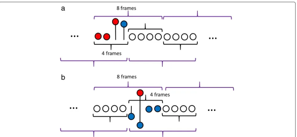
We will use Fig.4to explain the mechanism for iden-tifying the starting (Fig.4a) and ending (Fig. 4b) points. These two figures show the observation frames. To deter-mine the starting and ending points, the speech signal is observed in segments of eight frames with an overlap of four frames. The rules for identifying the starting and ending points are as follows:
(i) To identify a starting point, we consider eight frames at once and check the former four frames, as shown in Fig.4a. We observe these frames to find a frame that has the local maximum second derivative followed by a positive first derivative in the successive frame. When this pattern holds, such frame becomes a starting point candidate. This process continues for the successive eight frames with an overlap of four frames from the previous observation.
(ii) To identify an ending point, we consider eight frames at once and check the subsequent four frames, as shown in Fig.4b. We observe these frames to find a frame that has the combination of a local minimum first derivative and a local maximum second derivative that is preceded by at least one negative first derivative. When this pattern holds, such frame becomes an ending point candidate. This process continues for the successive eight frames overlapped with four frames from the previous observation.
The above two processes continue until the last observa-tion frames have been examined.
The starting and ending point candidates that are found based on rules (i) and (ii) are marked by the simple binary number of one. Figure5bshows the starting and ending point candidates of the speech signal. We then simply add
the binary ones between the starting and ending points to obtain masks, as shown in Fig.5c.
The masks, however, may cause misjudgments for non-speech periods because such masks do not carry informa-tion coming from the amplitude of the observed signal. To minimize such misjudgment, we attempt to remove values of “one” coming from the signal parts when the amplitudes are relatively small simply by multiplying the raw spectra expressed in decimal by the masks. Here-after, the output of this process is referred to as speech period candidates. The result of the process is shown in Fig. 5d. These speech period candidates, together with the log power spectra from Eq. (2), become input for the DNN. The same signal that is smeared by factory noise is shown in Fig. 6a. Figure6d shows the speech period candidates for the noisy signal smeared with factory noise (−5 dB).
2.2 DNN-based VAD
DNNs have been shown to be effective in various speech applications, including the detection of speech periods, as shown in [22]. According to [33], a DNN is a con-ventional multilayer perceptron (MLP) with many hidden layers. For simplicity, for anL+1-layer DNN, the input layer is regarded as layer 0, and the output layer is consid-ered layerL. In the firstLlayers, an activation vectorais obtained as follows:
a=f
z
=f
Wa−1+b
, for 0< <L. (6) wherez∈RN×1is an excitation vector,W∈RN×N−1 is a weight matrix,b ∈ RN×1is a bias vector, andN ∈
Ris the number of neurons in layer.f(.) :∈ RN×1 →
RN×1is an activation function applied to the excitation vector element-wisez. Here, the sigmoid function
σ(z)= 1
1+e−z (7)
is used.
In the input layer,a0 = P(m,k) ∈ RN0×1denotes the input feature vector of the DNN, whereP(m,k)denotes the log power spectra and the speech period candidates. P(m,k)is used as a learning instance and is mapped onto the correct speech periods that are identified during the training process.
In the output layer for classification tasks such as VAD, each output neuron represents a class i ∈ {1,. . .,C}, where C = NL is the number of classes. In the output
layer, a softmax function is added as a linear classifier for VAD:
aLi =softmaxi
zL= e
zLi
C
j=1ez
L J
, (8)
wherezLi is anith element of the excitation vectorzL. The value of theith output neuron aLi represents the probabil-ityPdnn(i|P)that the observationP(m,k)belongs to class
i(speech or non-speech).
The training process for the DNN mentioned above consists of two stages. First, a greedy layer-wise unsuper-vised learning procedure is performed as the pre-training stage. Next, fine-tuning is performed on the entire net-work [34]. The DNN considered in this study is composed of five layers of restricted Boltzmann machines (RBMs), which consist of visible and hidden units. Here, Bernoulli
(visible)–Bernoulli (hidden) RBMs, i.e., v ∈ {0, 1} and
h ∈ {0, 1}, are used. Once the learning process has been completed for an RBM, the activity values of its hidden units can be used as thefeature input for train-ing the next RBM [35]. A contrastive divergence algo-rithm is used in the pre-training stage to approximate the gradient of the negative log likelihood of the data with respect to the RBM’s parameters [36]. After the layer-by-layer pre-training stage, a backpropagation technique is applied throughout the entire net to fine-tune the weights to obtain optimal results [37]. Because the VAD output consists of two classes (i.e., speech and non-speech), the DNN-based VAD output for each frame is a binary vector whose elements are determined as follows:
ym=aL=
1, if speech is at framem, and
0, otherwise. (9)
The DNN outputs trains of 1s (ones) representing the speech periods.
3 Experimental results and discussion 3.1 Experimental setup
In the experiments, we use 99 speech files from the ASJ Continuous Speech Corpus for Research vol. 2 [38]. These speech files are divided equally into three data sets. Then, we create three groups, each with 66 files for training (a combination of two data sets to obtain three distinct groups), and the rest of the speech files are used for eval-uation purposes. The objective of dividing the data is to evaluate the proposed method inside a different data set. To obtain noisy signals, the clean speech files are mixed with five types of noise, white, babble, factory, car, and pink, from NOISEX-92 [39]. Each noise signal is differ-ently selected for the speech files as well as SNRs of 10, 5, 0, and−5 dB. Thus, 21 sets of data are used to produce 1386 speech files for the training of each group.
In this work, the input signals are sampled at 8 kHz. The frame size is 20 ms, and the analysis window is a Hamming window with a 10-ms frame shift. After the RSF filtering process, the LPS-RSF is calculated for an individual sub-band using Eq. (3). Next, the first and second derivatives for each subband are calculated using Eqs. (4) and (5). These derivatives are used to obtain the starting and end-ing point candidates in accordance with rules (i) and (ii). After the conversion of the starting and ending point can-didates from the sparse representation to the masks, the masks are multiplied by the spectra, expressed in decimal form to obtain speech period candidates. Then, the DNN is applied to the speech period candidates in combination with the log power spectra derived from Eq. (2). This com-bination (i.e., the dynamic features) is fed to the DNN to obtain the final VAD decision regarding the speech peri-ods. The dynamic features are normalized to zero mean and unit variance in each dimension. To train the DNN,
we use five RBMs. These RBMs are stacked together, and the number of neurons for each RBM is 200, 200, 200, 200, and 100, in sequence. The learning rate is 0.0001, and the maximum number of epochs for both the pre-training and fine tuning stages is 200.
Note that, after determining the speech and non-speech periods, we did not perform any post processing, such as a VADhangover, because such processing is outside the scope of this paper.
3.2 Results and discussion
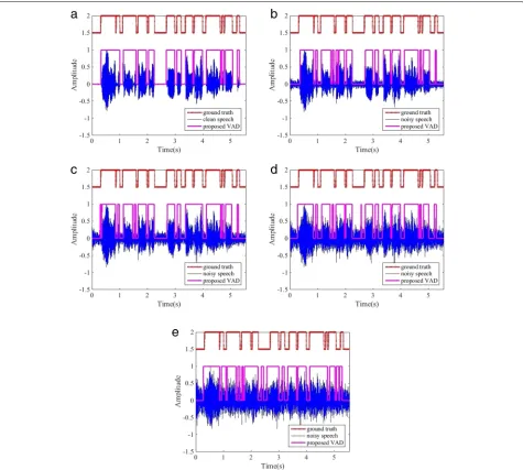
The VAD decisions on noisy signals smeared with fac-tory noise at various SNRs are shown in Fig.7. In Fig.7, the red dashed lines indicate the true speech and non-speech periods, whereas the solid magenta lines represent the generated VAD output. As shown in the figure, the output of the proposed VAD method is reasonably close to the ground truth.
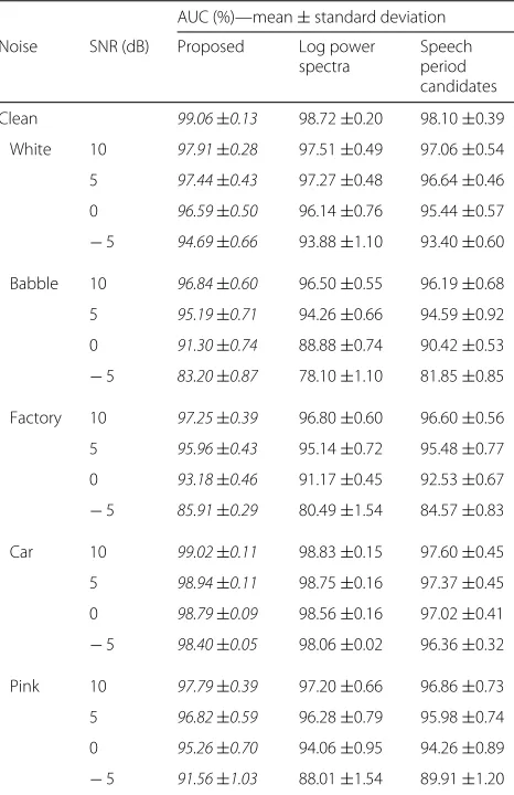
Table 1AUC (%) comparison between the proposed method and DNN-based VAD methods using speech period candidates and log power spectra as the baseline
AUC (%)—mean±standard deviation
Noise SNR (dB) Proposed Log power
spectra
Speech period candidates
Clean 99.06±0.13 98.72±0.20 98.10±0.39
White 10 97.91±0.28 97.51±0.49 97.06±0.54
5 97.44±0.43 97.27±0.48 96.64±0.46
0 96.59±0.50 96.14±0.76 95.44±0.57
−5 94.69±0.66 93.88±1.10 93.40±0.60
Babble 10 96.84±0.60 96.50±0.55 96.19±0.68
5 95.19±0.71 94.26±0.66 94.59±0.92
0 91.30±0.74 88.88±0.74 90.42±0.53
−5 83.20±0.87 78.10±1.10 81.85±0.85
Factory 10 97.25±0.39 96.80±0.60 96.60±0.56
5 95.96±0.43 95.14±0.72 95.48±0.77
0 93.18±0.46 91.17±0.45 92.53±0.67
−5 85.91±0.29 80.49±1.54 84.57±0.83
Car 10 99.02±0.11 98.83±0.15 97.60±0.45
5 98.94±0.11 98.75±0.16 97.37±0.45
0 98.79±0.09 98.56±0.16 97.02±0.41
−5 98.40±0.05 98.06±0.02 96.36±0.32
Pink 10 97.79±0.39 97.20±0.66 96.86±0.73
5 96.82±0.59 96.28±0.79 95.98±0.74
0 95.26±0.70 94.06±0.95 94.26±0.89
Fig. 8Improvement of VAD performance
To evaluate the effectiveness of the proposed method, we compare it with the DNN-based VAD method, which only utilizes the log power spectra, as the baseline of the evaluation.
To represent the performance of the proposed method, the receiver operation characteristic (ROC) curve, in which true positive rate (TPR) is plotted against false positive rate (FPR), is considered. The TPR, or sensitivity, and FPR are defined based on the number of true positives (TPs), false positives (FPs), true negatives (TNs), and false negatives (FNs) as follows [40]:
TPR= TP
TP+FN, and (10)
FPR= FP
FP+TN. (11)
To obtain a quantitative ROC value, the area under the curves (AUCs) are calculated. These AUCs are the main metric for evaluation.
Table 1 compares the average of the AUCs achieved by the DNN-based VAD methods using the log power spectra alone, the speech period candidates alone, and the proposed method. As shown in Table1, the proposed method may improve the performance of the DNN-based VAD method using the log power spectra for all cases. As shown in Fig.8, a relatively good improvement is obtained in low SNR cases. The highest improvement occurs at −5 dB, for example, the performance improves by 6.52% for babble noise at−5 dB.
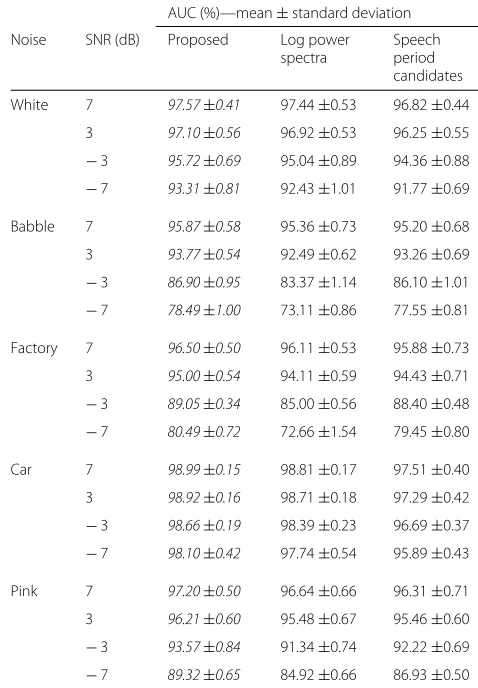
This method is also applied to SNR environments (7, 3, −3, and−7 dB) that are not known scenarios. The results for such SNR environments are shown in Table 2. The results in Tables1and2are from the known and unknown
Table 2AUC (%) comparison between the proposed method and DNN-based VAD methods using speech period candidates and log power spectra as the baseline for unknown SNR environments (7, 3,−3, and−7 dB)
AUC (%)—mean±standard deviation
Noise SNR (dB) Proposed Log power
spectra
Speech period candidates
White 7 97.57±0.41 97.44±0.53 96.82±0.44
3 97.10±0.56 96.92±0.53 96.25±0.55
−3 95.72±0.69 95.04±0.89 94.36±0.88
−7 93.31±0.81 92.43±1.01 91.77±0.69
Babble 7 95.87±0.58 95.36±0.73 95.20±0.68
3 93.77±0.54 92.49±0.62 93.26±0.69
−3 86.90±0.95 83.37±1.14 86.10±1.01
−7 78.49±1.00 73.11±0.86 77.55±0.81
Factory 7 96.50±0.50 96.11±0.53 95.88±0.73
3 95.00±0.54 94.11±0.59 94.43±0.71
−3 89.05±0.34 85.00±0.56 88.40±0.48
−7 80.49±0.72 72.66±1.54 79.45±0.80
Car 7 98.99±0.15 98.81±0.17 97.51±0.40
3 98.92±0.16 98.71±0.18 97.29±0.42
−3 98.66±0.19 98.39±0.23 96.69±0.37
−7 98.10±0.42 97.74±0.54 95.89±0.43
Pink 7 97.20±0.50 96.64±0.66 96.31±0.71
3 96.21±0.60 95.48±0.67 95.46±0.60
−3 93.57±0.84 91.34±0.74 92.22±0.69
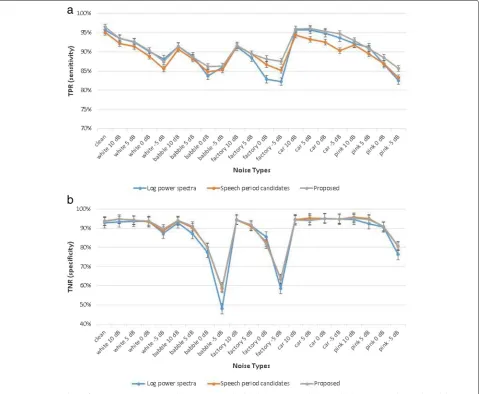
scenarios, respectively. Both tables show that the pro-posed method is able to enhance the usage of the log power spectra, even for the unknown SNR environments. To evaluate the effect of introducing the speech period candidates, we measure the TPR (sensitivity) and the true negative rate (TNR or specificity). Sensitivity gives the percentage of the frames that were correctly classified as speech from all the speech frames in the signal, and specificity gives the percentage of the frames that were correctly classified as non-speech from all the non-speech frames in the signal [41].
Figure 9 shows the mean TPR (sensitivity) and TNR (specificity). As shown in the figure, the proposed method has a high sensitivity and specificity for both the clean and noisy cases. Interestingly, the performance of the DNN-based VAD method using speech period candi-dates approaches and even outperforms the log power
spectra in finding speech, as shown in Fig. 9a, particu-larly for low SNRs and non-stationary cases. This fact may imply that the addition of speech period candidates is useful to find speech periods in low SNRs and non-stationary cases. Additionally, the specificity of speech period candidates is higher than the log power spectra as shown in Fig.9b. This fact may imply that the speech period candidates may improve the log power spectra for finding non-speech periods. Thus, the speech period can-didates may carry valuable information for judging speech and non-speech detection. In the proposed method, the addition of the speech period candidates is effective at improving the accuracy of the log power spectra at finding speech and non-speech periods, especially for low SNRs and non-stationary cases.
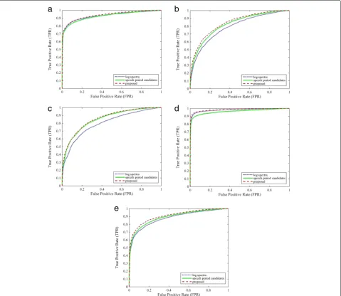
Figure 10 shows the ROC curves for the proposed method and the DNN-based VAD methods using speech
period candidates and log power spectra, respectively, at an SNR of−5 dB. As shown in the figure, the pro-posed method shows an advantage over the DNN-based VAD method using the log power spectra. The proposed method is effective for low SNR cases. In the cases of stationary noise, such as white and pink noise, the work-ing points of the proposed method are close to those of the DNN-based VAD method using the log power spec-tra. These methods achieve a high TPR and a low FPR. In the cases of non-stationary noise, such as babble and factory noise, the proposed method is less affected by the noise than the DNN-based VAD method using the log power spectra. The performance of the proposed method is superior to that of the DNN-based VAD method using the log power spectra mainly due to introducing dynamics
expressed by speech period candidates. To evaluate its effectiveness, the proposed method is also compared to other methods (Appendix2, Table 5).
In addition to the contribution of the speech period candidates, which may highlight dynamics, we attempt to find useful subbands for obtaining VAD decisions in the employed DNN. We evaluate which subbands have more valuable information than the others, by finding the similarity between the input (i.e., speech period candi-dates) and the VAD output. This similarity is evaluated by employing mutual information (MI), which aims to mea-sure whether the inputs are dependent on the associated labels (VAD output). According to [42], the MI between the discretized feature values aand the class labelsyis evaluated according to the formula
Table 3Subband (Hz) ranks using mutual information (MI)
Subband (Hz) ranks using MI
Noise SNR (dB) 1 2 3 4
Clean 187.5 218.75 156.25 312.5
White 10 187.5 218.75 156.25 250
5 187.5 218.75 156.25 250
0 187.5 218.75 156.25 250
−5 187.5 218.75 156.25 250
Babble 10 187.5 218.75 250 156.25
5 187.5 218.75 250 156.25
0 187.5 218.75 250 156.25
−5 187.5 218.75 250 156.25
Factory 10 187.5 218.75 156.25 250
5 187.5 218.75 156.25 250
0 187.5 218.75 250 156.25
−5 218.75 187.5 250 312.5
Car 10 187.5 218.75 156.25 250
5 187.5 218.75 312.5 250
0 187.5 218.75 250 312.5
−5 218.75 187.5 250 312.5
Pink 10 187.5 218.75 156.25 250
5 187.5 218.75 250 156.25
0 187.5 218.75 250 156.25
−5 187.5 218.75 250 156.25
MI=
a∈A
y∈Y
p(a,y)log p(a,y)
p(a)p(y)
, (12)
wherep(a,y)is a joint probability function ofaandyand
p(a)andp(y)are marginal probability distribution func-tions ofaandy, respectively. Here, the feature values,a,
are the input of the DNN (speech period candidates), and the class labels,y, are the VAD output. The larger the MI, the higher the dependency between the feature values, which represent speech period candidates for individual subbands, and the class labels (VAD output). Here, we rank the subbands according to their scores.
Table 3 shows the top 4 subband ranks using MI. As shown in Table 3, the top 4 ranks for clean, and noisy signals show a similar tendency for frequency bins 6, 7, 8, and 9 (156.25 Hz, 187.5 Hz, 218.75 Hz, and 250 Hz). Such subband may play some roles in obtain-ing the VAD decision in the proposed method. To clar-ify this, we perform experiments in which the four top subband values in the proposed method are replaced with zeros, and the resulting VAD performance is shown in Fig.11.
As shown in Fig.11, at a high SNR, the performance of the proposed method is only slightly degraded when the subbands of 156.25 Hz, 187.5 Hz, 218.75 Hz, and 250 Hz are replaced by zeros. In low SNR cases, the subbands are polluted by noise. Consequently, the performance might be degraded, and this degradation worsens when these top 4 subbands are not utilized. In contrast, when the four lowest subband values are replaced by zeros, the output accuracy can still be maintained. These results indicate that the top 4 subbands have a relatively important role in the decision-making process of the proposed method. We observe that the information carried by these subbands may correspond to the average of F0 or its neighbors (the average F0 for the data is 179.97 Hz, the average F0 for male is 149.09 Hz and 210.84 Hz for female; the F0s are measured using STRAIGHT algorithm [43]). Thus, in the proposed method, the DNN may utilize information com-ing from the useful subbands which may correspond to F0 and its neighbors.
4 Conclusions
This study presents a DNN-based VAD method for improving the performance of VAD by introducing dynamics, which may be highlighted by speech period candidates. These candidates are derived from heuristic rules based on the first and second derivatives of the log power spectrum of the RSF output (LPS-RSF). The speech period candidates are calculated for individual subbands and are then input into a DNN together with the log power spectra to generate the VAD decision. To evalu-ate the performance of the proposed method, we perform experiments using clean and noisy speech signals smeared with five types of noise, namely, white, babble, factory, car, and pink, with SNRs of 10, 5, 0 and−5 dB. The pro-posed method effectively detects speech and non-speech periods. The experimental results show that the VAD per-formance based on log power spectra are improved after combining the log power spectra with the speech period candidates, particularly for noisy speech signals with low SNRs and non-stationary cases. The addition of dynam-ics expressed by the speech period candidates provides positive information that contributes to the detection of speech periods.
In this study, we also show that the DNN-based VAD utilizes subbands that may correspond to F0 and its neighbors. The VAD performance degrades when those subbands are eliminated. However, further stud-ies should be performed to analyze other factors that influence the behavior of the employed DNN. Moreover, we intend to make the proposed method work in real time.
Appendix 1: preliminary experiment
In the preliminary experiment, we compared DNN-based VAD methods using log power spectra and “hand-crafted” features that are frequently used in speech processing, i.e., MFCC, delta features, and delta-delta features. All of these features were input into the DNN using the same config-uration and parameters as mentioned in Section3. The MFCCs were calculated using the same window length of 20 ms and the same shift of 10 ms. We consider 13 MFCCs augmented with delta features and delta-delta features, resulting in 39 combined features.
As shown in Table 4, the DNN-based VAD performance that was achieved using the log power spectra is supe-rior to that achieved using the MFCCs and that using MFCCs in combination with their delta and delta-delta cepstra. The log power spectra features capture more detailed information in the time-frequency domain. Con-sequently, these features represent a variety of important information that may be related to the speech characteris-tics. In contrast, the MFCCs may suffer from information loss, which may occur due to the dimension reduction caused by the DCT compression. In the preliminary study,
the DNN-based VAD performance that was achieved using the MFCCs is slightly improved when temporal derivatives, i.e., delta and delta-delta features, are consid-ered in combination with the MFCCs. The enhancement achieved by using the MFCCs in combination with the delta and delta-delta cepstra implies that the dynamics that are expressed by delta and delta-delta cepstra play a role in improving the VAD performance.
Appendix 2: comparison to conventional methods To evaluate the effectiveness of the proposed method, we also compare it with four other methods presented in [8,11,12,44].
Table 5 shows the AUC results of the proposed method and the other methods. As shown in the table, the proposed method outperforms the other methods in [8,11,12,44] for both clean and noisy signals. The per-formance of the method in [12], which utilizes a statistical method, approaches the performance of the method in [11], which utilizes MFCCs and a Gaussian mixture model (GMM) as the classifier. Their performance worsens for non-stationary noise. Alternatively, the method in [44]
Table 4AUC (%) comparison between DNN-based VAD methods using log power spectra and MFCCs
AUC (%)—mean±standard deviation Noise SNR (dB) Log power
spectra
MFCCs MFCCs++
Clean 98.72±0.20 98.18±0.08 97.79±0.41
White 10 97.51±0.49 96.10±0.59 96.91±0.57
5 97.27±0.48 93.99±0.85 95.11±0.97
0 96.14±0.76 89.58±1.46 90.85±1.73
−5 93.88±1.10 81.43±1.11 82.42±1.53
Babble 10 96.50±0.55 92.71±0.92 93.51±0.77
5 94.26±0.66 87.24±1.03 87.73±0.89
0 88.88±0.74 77.78±0 .99 77.86±0.82
−5 78.10±1.10 65.72±1.40 65.59±1.40
Factory 10 96.80±0.60 95.16±0.79 96.04±0.74
5 95.14±0.72 91.60±1.23 92.55±1.06
0 91.17±0.45 84.19±1.23 84.81±1.13
−5 80.49±1.54 72.40±1.14 72.70±0.72
Car 10 98.83±0.15 98.34±0.23 98.26±0.32
5 98.75±0.16 98.22±0.34 98.23±0.35
0 98.56±0.16 97.91±0.44 98.08±0.40
−5 98.06±0.02 97.27±0.54 97.70±0.46
Pink 10 97.20±0.66 95.91±0.81 96.64±0.62
5 96.28±0.79 93.31±1.00 94.28±0.99
0 94.06±0.95 87.96±1.54 88.91±1.40
Table 5AUC (%) comparison between the proposed method and other methods (Ramirez et al. [8], Kinnunen et al. [11], Sohn et al. [12], and Segbroeck et al. [44])
AUC (%)—mean±standard deviation
Noise SNR (dB) Proposed Ramirez Kinnunen Sohn Segbroeck
Clean 99.06±0.13 71.03±1.02 95.65±0.43 88.48±1.45 84.57±1.21
White 10 97.91±0.28 74.09±1.50 93.65±1.05 93.32±0.50 79.63±0.24
5 97.44±0.43 73.57±1.36 93.02±1.31 87.84±0.50 77.75±0.34
0 96.59±0.50 72.33±1.24 91.06±1.59 77.34±1.14 75.21±0.67
−5 94.69±0.66 68.97±1.07 83.85±1.28 66.79±1.85 71.89±0.77
Babble 10 96.84±0.60 68.84±1.32 87.71±0.91 87.56±0.87 81.25±0.35
5 95.19±0.71 67.28±0.71 84.19±0.80 79.97±0.70 79.05±0.69
0 91.30±0.74 63.62±0.91 76.59±0.99 70.05±0.94 72.99±1.13
−5 83.20±0.87 59.37±1.01 66.73±1.52 60.33±0.93 62.71±1.25
Factory 10 97.25±0.39 70.35±1.85 88.12±1.73 88.04±0.67 81.19±0.96
5 95.96±0.43 67.54±1.57 84.42±1.67 79.55±0.85 78.99±1.06
0 93.18±0.46 62.78±1.53 77.70±1.07 67.15±0.82 74.67±0.87
−5 85.91±0.29 57.81±1.71 66.38±0.76 56.28±0.56 67.23±0.52
Car 10 99.02±0.11 69.06±1.60 94.62±0.36 91.56±1.29 84.46±0.96
5 98.94±0.11 68.27±1.32 93.64±0.80 92.15±0.83 84.38±0.96
0 98.79±0.09 68.50±1.02 92.42±0.40 92.41±0.34 84.08±0.91
−5 98.40±0.05 68.77±1.87 90.16±0.17 91.81±0.10 83.49±1.06
Pink 10 97.79±0.39 73.11±1.67 90.37±1.33 90.54±0.40 81.00±0.94
5 96.82±0.59 72.36±1.63 88.87±1.85 82.51±1.39 78.96±1.21
0 95.26±0.70 70.32±1.53 84.13±1.76 71.70±1.70 76.10±1.31
−5 91.56±1.03 65.69±1.40 74.46±1.36 62.81±1.82 71.78±1.04 The numbers in italics indicate the best results
can give better performance for non-stationary and low SNRs than the method in [8]. The proposed method is superior to that of the other methods because it uses the advantages of using a DNN with features as the input, i.e., speech period candidates and log power spectra.
Authors’ contributions
All authors read and approved the final manuscript.
Competing interests
The authors declare that they have no competing interests.
Publisher’s Note
Springer Nature remains neutral with regard to jurisdictional claims in published maps and institutional affiliations.
Received: 8 December 2017 Accepted: 15 August 2018
References
1. K. Sakhnov, E. Verteletskaya, B. Simak, Approach for energy-based voice detector with adaptive scaling factor. IAENG Int. J. Comput. Sci.36, 394 (2009) 2. F. Beritelli, S. Casale, G. Ruggeri, inProc. IEEE Int Conf on Acoustics, Speech,
and Signal Processing. Performance evaluation and comparison of ITU-T/ETSI voice activity detectors (IEEE, Salt Lake City, 2001), pp. 1425–1428
3. A. Benyassine, ITU-T Recommendation G. 729 Annex B: a silence compression scheme for use with G. 729 optimized for V. 70 digital simultaneous voice and data applications. IEEE Commun. Mag.35, 64–73 (1997)
4. S. Tong, N. Chen, Y. Qian, K. Yu, inProc. IEEE Int Conf On Signal Processing. Evaluating vad for automatic speech recognition (IEEE, Hangzhou, 2014), pp. 2308–2314
5. S. Graf, T. Herbig, M. Buck, G. Schmidt, Features for voice activity detection: a comparative analysis. EURASIP J. Adv. Sign. Process.2015, 91 (2015) 6. L.R. Rabiner, M.R. Sambur, An algorithm for determining the endpoints of
isolated utterances. Bell Labs Tech. J.54, 297–315 (1975)
7. R.V. Prasad, A. Sangwan, H.S. Jamadagni, M.C. Chiranth, R. Sah, V. Gaurav, inProc 7th Int Symp on Computers and Communications. Comparison of voice activity detection algorithms for VoIP (IEEE, Taormina-Giardini Naxos, 2002), pp. 530–535
8. J. Ramırez, J.C. Segura, C. Benıtez, A. De La Torre, A. Rubio, Efficient voice activity detection algorithms using long-term speech information. Speech Comm.42, 271–287 (2004)
9. K. Ishizuka, T. Nakatani, M. Fujimoto, N. Miyazaki, Noise robust voice activity detection based on periodic to aperiodic component ratio. Speech Comm.52, 41–60 (2010)
10. K. Pek, T. Arai, N. Kanedera, Voice activity detection in noise using modulation spectrum of speech: investigation of speech frequency and modulation frequency ranges. Acoust. Sci. Technol.33, 33–44 (2012) 11. T. Kinnunen, P. Rajan, inProc. IEEE Int Conf on Acoustic, Speech and Signal
12. J. Sohn, N.S. Kim, W. Sung, A statistical model-based voice activity detection. IEEE Signal Proc. Lett.6, 1–3 (1999)
13. A. Davis, S. Nordholm, R. Togneri, Statistical voice activity detection using low-variance spectrum estimation and an adaptive threshold. IEEE Trans. Audio Speech Lang. Process.14, 412–424 (2006)
14. T. Kinnunen, E. Chernenko, M. Tuononen, P. Fränti, H. Li, inProc Int. Conf. on Speech and Computer (SPECOM07). Voice activity detection using MFCC features and support vector machine, (Moscow, 2007), pp. 556–561 15. Q.H. Jo, J.H. Chang, J.W. Shin, N.S. Kim, Statistical model-based voice activity detection using support vector machine. IET Sign. Process.3, 205–210 (2009)
16. D. Enqing, L. Guizhong, Z. Yatong, Z. Xiaodi,Applying support vector machines to voice activity detection, Proc Int Conf on Signal Processing. (IEEE, Beijing, 2002), pp. 1124–1127
17. G. Ferroni, R. Bonfigli, E. Principi, S. Squartini, F. Piazza, inA deep neural network approach for voice activity detection in multi-room domestic scenarios. Proc Int Joint Conference On Neural Networks (IEEE, Killarney, 2015), pp. 1–8
18. X.L. Zhang, D. Wang, Boosting contextual information for deep neural network based voice activity detection. IEEE/ACM Trans. Audio Speech Lang. Process.24, 252–264 (2016)
19. F. Bie, Z. Zhang, D. Wang, T. Zheng, DNN-based voice activity detection for speaker recognition. CSLT Tech. Rep (2015). available onlinehttp:// www.cslt.org/mediawiki/images/c/c8/Dvad.pdf
20. A.R. Mohamed, G.E. Dahl, G. Hinton, inProc IEEE Int Conf on Acoustics, Speech and Signal Processing. Understanding how deep belief networks perform acoustic modelling (IEEE, Kyoto, 2012), pp. 4273–4276 21. M. Espi, M. Fujimoto, K. Kinoshita, T. Nakatani, Exploiting spectro-temporal
locality in deep learning based acoustic event detection. EURASIP J. Audio Speech Music Process.2015(1), 26 (2015)
22. N. Ryant, M. Liberman, J. Yuan, inINTERSPEECH 2013, 14th Annual Conference of the International Speech Communication Association, ed. by F. Bimbot, C. Cerisara, C. Fougeron, G. Gravier, L. Lamel, F. Pellegrino, and P. Perrier. Speech activity detection on youtube using deep neural networks, (Lyon, 2013), pp. 728–731.http://www.isca-speech.org/ archive/interspeech_2013
23. V.S. Mendelev, T.N. Prisyach, A.A. Prudnikov, Robust voice activity detection with deep maxout neural networks. Mod. Appl. Sci.9(8), 153 (2015)
24. X.L. Zhang, J. Wu, Deep belief networks based voice activity detection. IEEE Trans Audio Speech Lang. Process.21, 697–710 (2013)
25. L. Deng, J. Li, J. Huang, K. Yao, D. Yu, F. Seide, M. Seltzer, G. Zweig, X. He, J. Williams, Y. Gong, A. Acero, inProc IEEE Int Conf On Acoustics, Speech and Signal Processing. Recent advances in deep learning for speech research at microsoft, (IEEE, Vancouver, 2013), pp. 8604–8608
26. L. Deng, Dynamic speech models: theory, algorithms, and applications. Synth. Lect. Speech Audio Process.2(1), 1–118 (2006)
27. K. Fujioka, N. Hayasaka, Y. Miyanaga, N. Yoshida, Noise reduction of speech signals by running spectrum filtering. Syst. Comput. Jpn.37, 52–61 (2006)
28. N. Kanedera, T. Arai, H. Hermansky, M. Pavel, On the relative importance of various components of the modulation spectrum for automatic speech recognition. Speech Commun.28, 43–55 (1999)
29. H. Hermansky, N. Morgan, RASTA processing of speech. IEEE Trans. Speech Audio Process.2, 578–589 (1994)
30. L. Atlas, S.A. Shamma, Joint acoustic and modulation frequency. EURASIP J. Adv. Sign. Process.2003, 310–290 (2003)
31. T. Arai, M. Pavel, H. Hermansky, C. Avendano, Syllable intelligibility for temporally filtered LPC cepstral trajectories. J. Acoust. Soc. Am.105, 2783–2791 (1999)
32. Q. Zhu, N. Ohtsuki, Y. Miyanaga, N. Yoshida, inProc IEEE Int Symp on Communications and Information Technology. Robust speech analysis in noisy environment using running spectrum filtering (IEEE, Sapporo, 2004), pp. 995–1000
33. D. Yu, L. Deng,Automatic speech recognition A deep learning approach. (Springer, London, 2014)
34. H. Larochelle, Y. Bengio, J. Louradour, P. Lamblin, Exploring strategies for training deep neural networks. J. Mach. Learn. Res.10, 1–40 (2009) 35. G.E. Hinton, Learning multiple layers of representation. Trends Cogn. Sci.
11, 428–434 (2007)
36. M.A. Carreira-Perpinan, G.E. Hinton, On contrastive divergence learning. AISTATS.10, 33–40 (2005)
37. M.A. Keyvanrad, M.M. Homanyounpour, A brief survey on deep belief networks and introducing a new object oriented toolbox (DeeBNet). arXiv preprint arXiv:1408.3264. (2014).https://arxiv.org/abs/1408.3264
38. T. Kobayashi, S. Itabashi, S. Hayashi, T. Takezawa, ASJ continuous speech corpus for research. J. Acoust. Soc. Jpn.48, 888–893 (1992)
39. The Rice University, “Noisex-92 Database”.http://spib.linse.ufsc.br/noise. html. Accessed 22 Feb 2017
40. R.O. Duda, P.E. Hart, D.G. Stork,Pattern classification, 2nd edn. (New York, 2001)
41. M. Myllymäki, T. Virtanen, inProc 16th European Signal Processing Conference. Voice activity detection in the presence of breathing noise using neural network and hidden markov model (IEEE, Lausanne, 2008), pp. 1–5
42. J. Pohjalainen, O. Räsänen, S. Kadioglu, Feature selection methods and their combinations in high-dimensional classification of speaker likability, intelligibility and personality traits. Comput Speech Lang.29(1), 145–171 (2015)
43. H. Kawahara, I. Masuda-Katsuse, A. De Cheveigne, Restructuring speech representations using a pitch-adaptive time–frequency smoothing and an instantaneous-frequency-based F0 extraction: Possible role of a repetitive structure in sounds. Speech Commun.27(3), 187–207 (1999) 44. M.V. Segbroeck, A. Tsiartas, S. Narayanan, inProc INTERSPEECH 2013, 14th