CutIGA with basis function removal

(1)

R E S E A R C H A R T I C L E

Open Access

CutIGA with basis function removal

Daniel Elfverson, Mats G. Larson and Karl Larsson

∗

*_{Correspondence:}

[email protected]

Department of Mathematics and Mathematical Statistics, Umeå University, 90 187 Umeå, Sweden

Abstract

We consider a cut isogeometric method, where the boundary of the domain is allowed to cut through the background mesh in an arbitrary fashion for a second order elliptic model problem. In order to stabilize the method on the cut boundary we remove basis functions which have small intersection with the computational domain. We determine criteria on the intersection which guarantee that the order of convergence in the energy norm is not aﬀected by the removal. The higher order regularity of the B-spline basis functions leads to improved bounds compared to standard Lagrange elements.

Introduction

Background and earlier work

CutFEM and CutIGA, are methods where the geometry of the domain is allowed to cut through the background mesh in an arbitrary fashion, which manufactures so called cut elements at the boundary. This approach typically leads to some loss of stability and ill conditioning of the resulting stiﬀness matrix that must be handled in some way. Several approaches have been proposed:

• Gradient jump penalties or some related stabilization term, see [3] and [4].

• Adding a small amount of extra stiﬀness to each active element as is done in the ﬁnite cell method, see [7] and [12].

• Element merging where small elements are associated with a neighbor which has a large intersection. For DG methods see [11] and for CG methods see [1].

• Basis function removal where basis functions with support that has a small intersec-tion with the domain are removed. For the case of isogeometric spline spaces see [8].

For a general introduction to CutFEM we refer to the overview paper [4] and for an introduction to isogeometric analysis we refer to [6].

New contributions

We investigate the basis function removal approach based on simply eliminating basis functions that has a small intersection with the domain in the context of isogeometric analysis, more precisely we employ B-spline spaces of orderpwith maximal regularity

Cp−1. To this end we need to make the meaning of small intersection precise and our

©The Author(s) 2018. This article is distributed under the terms of the Creative Commons Attribution 4.0 International License (http://creativecommons.org/licenses/by/4.0/), which permits unrestricted use, distribution, and reproduction in any medium, provided you give appropriate credit to the original author(s) and the source, provide a link to the Creative Commons license, and indicate if changes were made.

(2)

guideline will be that we should not lose order in a given norm. In particular, we consider the error in the energy norm and show that we may remove basis functions with suﬃciently small energy norm and still retain optimal order convergence.

We also quantify the meaning of a basis function with suﬃciently small energy norm in terms of the size of the intersection between the support of the basis function and the domain. In order to measure the size of the intersection we consider a corner inside the domain and we letδi,i=1,. . ., dwithdthe dimension, be the distance from the corner

to the intersection of edgeEiwith the boundary. If there is no intersectionδi = h. We

then identify a condition onδiin terms of the mesh parameterhwhich guarantees that

we have optimal order convergence in the energy norm. The energy norm of the basis functions may be approximated by the diagonal element of the stiﬀness matrix and we propose a convenient selection procedure based on the diagonal elements in the stiﬀness matrix which is easy to implement.

We also derive the condition onδicorresponding to theW_∞1 norm, which will be tighter

since the norm is stronger and here we also need the continuity of the derivative of the basis functions. We discuss the approach in the context of standard Lagrange basis function where we note that we get much a tighter condition onδiin the energy norm and in the

W_∞1 norm we ﬁnd that it is not possible to remove basis functions.

We impose Dirichlet conditions weakly using nonsymmetric Nitsche, which is coercive by deﬁnition. Since the energy norm used in the nonsymmetric Nitsche method does not control the normal gradient on the Dirichlet boundary we do however need to add a standard least squares stabilization term on the elements in the vicinity of the boundary. Note that this term is element wise in contrast to the stabilization terms usually used in CutFEM.

When symmetric Nitsche is used to enforce Dirichlet boundary conditions stabilization appears to be necessary to guarantee that a certain inverse estimate holds. This bound is not improved by the higher regularity of the splines and will not be enforced in a satisfactory manner by basis function removal.

Outline

In “The model problem and method” section we introduce the model problem and the method, in Chapter 3 we derive properties of the bilinear form, define the interpolation operator, define the criteria for basis function removal, derive error bounds, and quantify δ in terms ofhfor various norms, and finally in “Numerical results” section we present some illustrating numerical examples.

The model problem and method Model problem

Let be a domain in Rd _{with smooth boundary} _∂ _{and consider the problem: ﬁnd}

u:→Rsuch that

−u=f in (1)

u=gD on∂D (2)

(3)

For suﬃciently regular data there exists a unique solution to this problem and we will be interested in higher order methods and therefore we will always assume that the solution satisﬁes the regularity estimate

uHs₍₎1 (4)

fors ≥ 2. Here and belowa bmeans that there is a positive constantC such that

a≤Cb.

The finite element method The B-spline spaces

• LetT_h,h ∈ (0, h0], be a family of uniform tensor product meshes inRd with mesh parameterh.

• LetVh = Cp−1Qp(Rd) be the space of Cp−1tensor product B-splines of order p

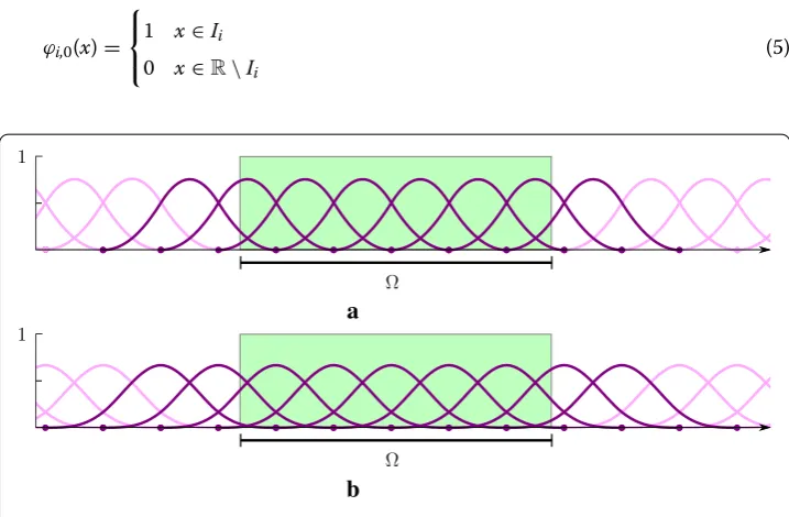
deﬁned onTh. LetB= {ϕi}i∈Ibe the standard basis inVh, whereIis an index set.

• LetB= {ϕ ∈B : supp(ϕ)∩ = ∅}be the set of basis functions with support that intersects. LetIbe an index set forB. LetVh = span{B}and letTh = {T ∈ Th :

T ⊂ ∪_ϕ_∈Bsupp(ϕ)}. An illustration of the basis functions in1Dis given in Fig.1. • LetB=Ba∪Brbe a partition into a setBaof active basis functions which we keep

and a setBrof basis functions which we remove. LetI=Ia∪Irbe the corresponding

partition of the index set. LetV_h,a=span{Ba}be the active ﬁnite element space.

Remark 1 To construct the basis functions inVhwe start with the one dimensional lineR

and deﬁne a uniform partition, with nodesxi=ih,i∈Z, wherehis the mesh parameter,

and elementsIi=[xi−1, xi). We deﬁne

ϕi,0(x)=

⎧ ⎨ ⎩

1 x∈Ii

0 x∈R\Ii

(5)

a

b

(4)

The basis functionsϕi,pare then deﬁned by the Cox-de Boor recursion formula

ϕi,p=

x−xi

x_i+p−xiϕi,p−1

(x)+ xi+p+1−x

x_i+p+1−xi+1ϕi+1,p−1

(x) (6)

we note that these basis functions areCp−1and supported on [xi, xi+p+1] which corre-sponds top+1 elements, see Fig.1. We then deﬁne tensor product basis functions inRd of the form

ϕi1,...,id(x)= d

k=1

ϕik(xk) (7)

The nonsymmetric method Finduh,a∈Vh,asuch that

A_h(u_h,a, v)=L_h(v) v∈V_h,a (8)

The forms are deﬁned by

A_h(v, w)=a_h(v, w)+τh2(v,w)_T_h,D_∩ (9)

Lh(v)=lh(v)+τh2(f,v)Th,D∩ (10)

where

ah(v, w)=(∇v,∇w)−(n· ∇v, w)∂D+(v, n· ∇w)∂D+βh−

1₍_{v, w}₎

∂D (11)

lh(v)=(f, v)+(gN, v)∂N +(gD, n· ∇v)∂D+βh−

1₍_g

D, v)∂D (12)

with positive parametersβandτ. Furthermore, we used the notation

(v, w)Th,D∩=

T∈Th,D

(v, w)T∩ (13)

whereTh,D⊂This deﬁned by

Th,D=Th(Uδ(∂D))= {T ∈Th:T ∩Uδ(∂D)= ∅} (14)

and

U_δ(∂D)= ⎛

⎝

x∈∂D

B_δ(x)

⎞

⎠_∩ (15)

withδ ∼ handB_δ(x) the open ball with centerxand radiusδ. We note that it follows from (14) thatU_δ(∂D)⊂Th,D.

Galerkin orthogonalityIt holds

A_h(u−u_h, v)=0 ∀v∈V_h (16)

Remark 2 In practice, Th,D may be taken as the set of all elements that intersect the

(5)

Remark 3 (The Symmetric Method)The symmetric version of (8) takes the form: ﬁnd

uh,a∈Vh,asuch that

ah,sym(uh,a, v)+sh,sym(uh,a, v)=lh,sym(v) v∈Vh,a (17)

a_h,_sym(v, w)=(∇v,∇w)−(n· ∇v, w)_∂_D −(v, n· ∇w)_∂_D +βh−1(v, w)_∂_D (18)

sh,sym(v, w)=γh2p−1

[DpnFv],[D p nFw]

FD,h (19)

lh,sym(v)=(f, v)+(gN, v)∂N −(gD, n· ∇v)∂D +βh−

1₍_g

D, v)∂D (20)

whereβandγ are positive parameters,Fh,Dis the set of interior faces which belong to an

element inTh(∂D), andDnF =nF· ∇is the directional derivative normal to the faceF. The stabilization termsh,symprovides the control

∇v2_T

h(∂D)∇v

2

+ v2sh,sym v∈Vh (21)

where we note that we indeed obtain control on the full elements T ∈ Th(∂D). The

control (21) is employed in the proof of the coercivity ofAhin the symmetric case. More

precisely, (21) is used as follows

hn· ∇v2_∂_D ∇v2_T

h(∂D)∇v

2

+ v2sh,sym (22)

where we used an inverse inequality in the ﬁrst estimate

In the symmetric formulation we stabilize to ensure that coercivity holds and this sta-bilization also implies that the resulting linear system of equations is well conditioned. Therefore, in the symmetric case, we do not employ basis function removal on the Dirich-let boundary.

Error estimates Basic properties ofA_h

Energy normDeﬁne the norms

|||v|||2_h= ∇v2 +h−1v2_∂

D+τh

2_v2

Th,D∩ (23)

|||v|||2_h,= ∇v2 +h−1v2_∂

D+τh

2_v2

Th,D∩+hn· ∇v

2

∂D (24)

CoercivityForβ >0 the formA_his coercive

|||v|||2_hAh(v, v) v∈V+Vh (25)

whereV =H2(). This result follows directly from the deﬁnition and the fact that the parametersτ ≥0 andβ >0.

ContinuityThe formA_his continuous

(6)

Proof First we note that

A_h(v, w)=(∇v,∇w)−(n· ∇v, w)_∂_D

+(v, n· ∇w)_∂_D +βh−1(v, w)_∂_D+τh2(v,w)_T_h,D_∩ (27) |(∇v,∇w)−(n· ∇v, w)_∂_D| + |||v|||h|||w|||h, (28)

We proceed with an estimate of the ﬁrst term on the right hand side. To that end let χ :→[0,1] be a smooth function such that

⎧ ⎪ ⎪ ⎨ ⎪ ⎪ ⎩

χ=1 on∂D

supp(χ)⊂U_δ(∂D) ∇χL∞₍_U_δ₍_∂_D₎₎ δ−1

(29)

whereU_δ(∂_δ) is deﬁned in (15). Splitting the term (∇v,∇w)usingχand then applying Green’s formula for the term in the vicinity of∂Dfollowed by some obvious bounds give

(∇v,∇w)−(n· ∇v, w)_∂_D

=(∇v,(1−χ)∇w)+(∇v,χ∇w)−(n· ∇v,χw)_∂_D (30)

=(∇v,(1−χ)∇w)−(∇ ·(χ∇v), w) (31)

=(∇v,(1−χ)∇w)−(∇χ· ∇v, w)−(χv, w) (32)

∇v∇w+δ−1∇vU_δ(∂D)wUδ(∂D)+ vUδ(∂D)wUδ(∂D) (33)

where we in (31) assumev∈H2() which holds ifVhis a space ofCp−1tensor product

B-splines of orderp≥2. Next using the bound

w2_U_δ₍_∂

D)δw

2

∂D+δ

2_∇_w2

Uδ(∂D) (34)

see [5], we conclude that

(∇v,∇w)−(n· ∇v, w)_∂_D (35) ∇v∇w+δ−1∇vU_δ(∂D)(δw

2

∂D+δ

2_∇_w2

Uδ(∂D))

1/2 ₍₃₆₎

+ vU_δ(∂D)(δw∂D+δ

2_∇_w2

Uδ(∂D))

1/2 ₍₃₇₎

∇v∇w+ ∇vU_δ₍_∂_D₎(δ−1w2_∂

D+ ∇w

2

Uδ(∂D))

1/2 ₍₃₈₎

+δvU_δ(∂D)(δ−

1_w

∂D+ ∇w

2

Uδ(∂D))

1/2 ₍₃₉₎

(∇v2+ ∇v2_U_δ₍_∂

D)+δ

2_v2

Uδ(∂D))

1/2 ₍₄₀₎

×(∇w2+δ−1w2_∂_D+ ∇w2_U_δ₍_∂

D))

1/2 ₍₄₁₎

(∇v2+δ2v2_U_δ₍_∂

D))

1/2 ₍₄₂₎

×(∇w2+δ−1w2_∂_D)1/2 (43)

Finally, choosingδ∼hand using the fact thatU_δ(∂D)⊂Th,Dwe obtain

(∇v,∇w)−(n· ∇v, w)_∂_D |||v|||h|||w|||h, (44)

(7)

Interpolation error estimates

Definition of the interpolantThere is an extension operatorE:W_qk()→W_qk(Rd),k≥0 andq≥1, such that

Ev_Wk

q(Rd)vWqk() (45)

see [9]. Deﬁne the interpolant by

πh:Hs()u→πCl,h(Eu)∈Vh (46)

whereπCl,his a Clement type interpolation operator onto the spline space. We have the

expansion

πh(Ev)=

ϕi∈I

(πh(Ev))iϕi (47)

where (πh(Ev))iis the coeﬃcient corresponding to basis functionϕi. We deﬁne the

inter-polant on the active and removed ﬁnite element spaces by

πh,av=

ϕi∈Ia

(πh(Ev))iϕi (48)

and

πh,rv=

ϕi∈Ir

(πh(Ev))iϕi (49)

We then have

πh(Ev)=πh,a(Ev)+πh,r(Ev) (50)

Below we simplify the notation and writev=Evandπh(Ev)=πhv.

Basis function removal conditionLetBr, with corresponding index setIr, be such that

i∈Ir

|||ϕi|||2_h,tol2 (51)

Selection procedureTo determineBrwe may thus compute|||ϕi|||h,,i∈I, sort the basis

functions in increasing order and then simply add functions toIras long as (51) is satisﬁed.

If we wish to avoid computing|||ϕi|||h,we may use the directly available diagonal values

Ah(ϕi,ϕi) of the stiﬀness matrix as approximations.

Lemma 1 (Interpolation error estimate)Letπh,abe defined by (48) with B=Ba∪Brsuch

that Brsatisfies (51), then

(8)

Proof Using the identityπ_hv=πh,av+πh,rvand the triangle inequality

|||v−π_h,av|||2_h,|||v−π_hv|||2_h,+ |||π_h,rv|||2_h, (53) h2pv2_Hp+1₍₎+ |||πh,rv|||2h, (54)

by standard spline interpolation results [2]. To estimate the second term on the right hand side we introduce the scalar product

v, wh,=(∇v,∇w) + h(n· ∇v, n· ∇w)_∂_D + h−1(v, w)_∂_D + h2(v,w)_T_h,D_∩ (55)

associated with the norm||| · |||h,. Expandingπh,rvin the basisBrwe get

|||πh,rv|||2h,=

i,j∈Ir

(π_hv)i(πhv)jϕi,ϕjh, (56)

≤

i∈Ir

j∈Ir

δij|(π_hv)i| |(π_hv)j| |||ϕi|||h,|||ϕj|||h, (57)

≤

i∈Ir

j∈Ir δij

2 |(πhv)i| 2_|||_ϕ

i|||h,+δ₂ij|(πhv)j|2|||ϕj|||h, (58)

=

i∈Ir

⎛

⎝

j∈Ir δij

⎞

⎠_|(π_hv)i|2|||ϕi|||2_h, (59)

πhv2_L∞₍_N

h())

⎛

⎝

i∈Ir |||ϕi|||2

h, ⎞

⎠ (60)

v2_Hp+1₍₎tol2 (61)

Here

• We deﬁned

δij= ⎧ ⎨ ⎩

1 if supp(ϕi)∩supp(ϕj)= ∅

0 if supp(ϕi)∩supp(ϕj)= ∅

(62)

and we have the bound

j∈Ir

δij≤(2p+1)d (63)

• We used theL∞(N_h()) stability of the interpolantπ_hand then theL∞stability of the extension operator and ﬁnally the Sobolev embedding theorem

πhvL∞(Nh())vL∞(Nh())vL∞()vHp+1() (64)

(9)

Error estimate

We have the following error estimate.

Theorem 1 Let uh,a be the solution to (8) with Vh,a = span{Ba}the active spline space,

Vh=span{B}the full spline space, and B=Ba∪Br, where Brsatisfies (51) with tol∼hp,

then

|||u−uh,a|||hhpuHp+1₍₎ (65)

Proof Using coercivity (25), Galerkin orthogonality (16), and continuity (26), we obtain

|||u−uh,a|||2hAh(u−uh,a, u−uh,a) (66)

=A_h(u−u_h,a, u−π_h,au) (67)

|||u−uh,a|||h|||u−πh,au|||h, (68)

Thus we arrive at

|||u−uh,a|||h|||u−πh,au|||h, (69)

which together with the interpolation error estimate (52) completes the proof of (65).

Remark 4 Note that if we takeτ = 0, i.e. we use the method without least squares stabilization in the vicinity of the Dirichlet boundary. We may still derive an error estimate as follows

∇(u−uh,a)2+ u−uh_∂2 _D Ah(u−uh,a, u−uh,a) (70)

=A_h(u−u_h,a, u−π_h,au) (71)

|||u−uh,a|||h|||u−πh,au|||h, (72)

Now we note that

|||u−uh,a|||2h= ∇(u−uh,a)2+ u−uh2_∂_D+h2(u−uh,a)2Th,D∩ (73) = ∇(u−uh,a)2+ u−uh_∂2 _D+h2f −uh,a2Th,D∩ (74)

and thus we obtain the bound

∇(u−uh,a)2+ u−uh2∂D h

2p_u2

Hp+1₍₎+h2f −uh,a2_T_h,D∩ (75)

(10)

Bounds in terms of the geometry of the cut elements

In this section we derive a criterion in terms of the geometry of the cut support of the basis function which implies (51). This criterion will in general not be used in practice but it provides insight into the eﬀect of the higher order regularity of the B-splines.

Assuming that there areh−(d−1)such elements we have the estimate

i∈Ir

|||ϕi|||2_h,h−(d−1)max i∈Ir

|||ϕi|||2

h, (76)

and settingtol∼hpwe get

max

i∈Ir

|||ϕi|||2_h,hd−1tolh2p+d−1 (77)

and we may deﬁneBr as all basis functionsϕ∈Bsuch that

|||ϕ|||2

h,hd−1tolh2p+d−1 (78)

Let us for simplicity consider a basis functionϕ such that supp(ϕ)⊂ ∂D = ∅, i.e. a

basis function that reside on the Neumann part of the boundary. In this case|||ϕ|||h, =

∇ϕsupp(ϕ)∩and thusϕ∈Brif

∇ϕ2

supp(ϕ)∩h2p+d−1 (79)

The 1D case: energy normLet = [0,1] and consider a basis functionϕ with support [X0, X1] such thatX0∈[0,1] and supp(ϕ)∩[0,1]=[X0,1] is an interval of lengthδ. Then forδsmall enough we have

ϕ(x)=

_x

h p

, |Dϕ(x)|2= p 2

h2

_x

h 2(p−1)

(80)

up to constants and in local coordinates with origoX0, and

Dϕ2=

_δ 0 p2 h2 _x h 2(p−1)

= p

h p

2p−1

δ

h 2p−1

(81)

Condition (79) thus takes the form

p h

p

2p−1

_δ

h 2p−1

h2p+d−1 =⇒ δ

h h

2p+1

2p−1 ₍₈₂₎

For Lagrange basis functions we instead have|Dϕ(x)| ∼h−1and we therefore obtain the condition

δh−2h2p+d−1 =⇒ x

δ h2p+1 (83)

(11)

a b c d

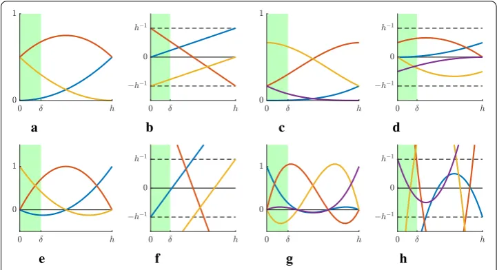
e f g h

Fig. 2 B-spline (top row) and Lagrange (bottom row) basis functions of orderp=2,3 in a1Delement intersecting. Note that gradient of the blue B-spline basis functions isO(h−1(_hδ)p−1) withinwhile the gradient of Lagrange basis functions isO(h−1) regardless ofp.aC1Q2basis.bC1Q2gradient.cC2Q3basis.d C2_Q3_gradient._e_Q2_basis._f_Q2_gradient._g_Q3_basis._h_Q3_gradient

The 1D case: max normThe diﬀerence between the B-splines and Lagrange basis functions is even more drastic if we consider instead evaluating the max norm of the derivative. Then for B-splines we have

DϕL∞_(supp(_ϕ₎_∩₎h−1

δ

h _p−1

(84)

while for Lagrange basis functions

DϕL∞_(supp(_ϕ₎_∩₎h−1 (85)

which in the latter case can not be controlled by decreasingδ, see Fig.2. Thus for Lagrange basis functions we get a pointwise error of orderh−1if we remove a basis function while for quadratic and higher order B-splines we may retain optimal order local accuracy by choosing

δ

h h

p+1

p−1 ₍₈₆₎

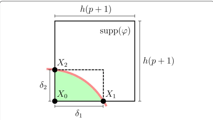
The 2D case: energy norm We now extend our calculation to the 2D case. The higher dimensional case can be handled using a similar approach. LetX0be a vertex of supp(ϕ) which reside in the interior of. Let{ei}d_i=₁be an orthonormal coordinate system centered

atX0and with basis vectorsei, and coordinatesxi, aligned with the edges{Ei}d_i₌₁of supp(ϕ)

which originates atX0, see Fig.3. Using the local coordinates in the vicinity ofX0we have the expansions

ϕ(x1, x2)=

_x₁ h

px2

h p

(87)

|∇ϕ(x1, x2)|2= 1

h2

_x₁ h

2p−2_x₂

h 2p

+ 1

h2

_x₁ h

2p_x₂

h 2p−2

(12)

Fig. 3 Illustration of the geometric quantities used in intersection conditions (51) in energy norm and (96) in max norm

Letδi= Xi−X0_Rdbe the distance from the vertexX0to the intersectionXiof edgeEi

with the boundary∂. Assume that

supp(ϕ)∩⊂[0,δ1]×[0,δ2] (89)

Integrating over [0,δ1]×[0,δ2] we obtain

_δ₁

0

_δ₂

0 |∇ϕ| 2

_δ

1

h

2p−1_δ 2

h 2p+1

+

_δ

1

h

2p+1_δ 2

h 2p−1

(90)

Condition (79) thus takes the form

_δ

1

h

2p−1_δ 2

h 2p+1

+

_δ

1

h

2p+1_δ 2

h 2p−1

h2p+d−1 (91)

which implies

δ1

h h

δ2

h ₋2p−1

2p+1

and δ2

h h

δ1

h ₋2p−1

2p+1

(92)

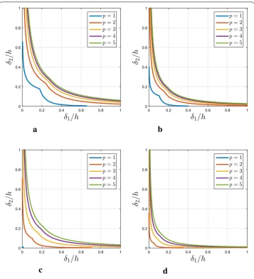
See Fig.4for an illustration of this condition.

The 2D case: max norm Starting from the expansion (88) and observing that for small enough δ parameters |∇ϕ|2 is increasing when we move out from the vertex. Using assumption (89) we thus conclude that

∇ϕL∞_(supp(_ϕ₎_∩|∇ϕ(δ1,δ2)| (93)

We have

∇ϕ(x1, x2)=

p h

_x₁ h

_p−1_x₂

h p , p h _x₁ h

px2

h _p−1

(13)

a

b

d

c

Fig. 4 Illustrations of the basis function intersection condition (51) in energy norm and (96) in max norm for splines of polynomial orderp=1,2,. . .,5.aEnergy norm,h=0.1.bEnergy norm,h=0.05.cMax norm, h=0.1.dMax norm,h=0.05

Settingx1=δ1andx2=δ2we get the conditions

p h

_δ

1

h

p−1_δ 2

h

p

hp and p

h

_δ

1

h

p_δ

2

h p−1

hp (95)

which we may write in the form

δ1

h

1

ph

p+1

p

δ2

h ₋p−1

p

and δ2

h

1

ph

p+1

p

δ1

h ₋p−1

p

(96)

(14)

Numerical results Linear elasticity

While we for simplicity use the Poisson model problem in the above analysis the same analysis holds also for other second order elliptic problems which may be of more practical interest. We therefore in the numerical results apply our ﬁndings to the linear elasticity problem: ﬁnd the displacementu:→Rdsuch that

−σ(u)· ∇ =f in (97)

σ(u)·n=gN on∂N (98)

u=gD on∂D (99)

where the stress and strain tensors are deﬁned by

σ(u)=2μ(u)+λtr((u)), (u)= 1 2

u⊗ ∇ + ∇ ⊗u (100)

with Lamé parametersλandμ;f,gN,gDare given data;a⊗bis the tensor product of

vectorsaandbwith elements (a⊗b)ij=aibj.

The nonsymmetric method for linear elasticty Findu_h,a∈[V_h,a]d_{such that}

A_h(u_h,a, v)=L_h(v) v∈[V_h,a]d (101)

A_h(v, w)=a_h(v, w)+τh2((v)· ∇,(w)· ∇)_T_h,D_∩ (102)

Lh(v)=lh(v)+τh2(f,(v)· ∇)Th,D∩ (103)

where

ah(v, w)=(σ(v),(w))−(σ(v)·n, w)∂D +(v,σ(w)·n)∂D+βh−

1₍_{v, w}₎

∂D (104)

lh(v)=(f, v)+(gN, v)∂N +(gD,σ(v)·n)∂D+βh−

1₍_g

D, v)∂D (105)

with positive parametersβandτ. Furthermore, the energy norm is deﬁned

|||v|||2_h=(σ(v),(v))+h−1v2_∂

D+τh

2₍_v₎_{· ∇}2

Th(∂D)∩ (106)

(15)

a

b

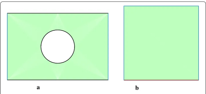
Fig. 5 Geometries in the two model problems. Boundaries with non-homogeneous Neumann conditions are indicated in blue and Dirichlet boundaries are indicated in red.aNeumann problem.bManufactured problem

A manufactured problemTo numerically estimate convergence rates we use the following manufactured problem from [10]. The geometry and the solution is given by

=[0,1]2, ∂D= {x∈[0,1], y=0}, ∂N =∂\∂D (107)

u(x, y)=[−cos(πx) sin(πy),sin(πx/7) sin(πy/3)]/10 (108)

see Fig.5b. Assuming a linear isotropic material with the material parameters of steel we deduce expressions for the input dataf,gN andgD. Note that while this problem does

include a Dirichlet boundary ∂D we in our current implementation neglect the least

squares term in the vicinity of∂D, i.e. we chooseτ =0.

Illustration of the selection procedure

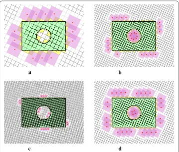
We utilize the selection procedure based on the stiﬀness matrix proposed in “Interpolation error estimates” section. Some realizations of this selection are visualized in Fig.6where we note that the selection becomes more restrictive as the mesh size decreases. This is a natural eﬀect as the selection procedure is developed to ensure optimal approximation properties of the active spline spaceVh,a. We also note that when increasing spline order

more basis functions are removed when using the same constant in the tolerancetol=chp. This can also be seen in Fig.7where we investigate how the choice of this constant eﬀects the number of removed basis functions. In Fig.8we note that the use of basis removal is quite eﬀective and also gives better quality stresses along the boundary.

Convergence

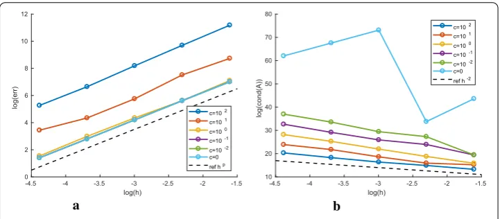
To estimate the convergence we use the manufactured problem described in “Linear elasticity” section and the cut situations are induced by rotating the background grid π/7 radians as illustrated by the mesh with removed basis functions in Fig.9together with the corresponding numerical solution. In Fig.10a we present convergence studies in energy norm for various choices of the constantc in the tolerancetol = chp×√E

(16)

a

b

d

c

Fig. 6 Four realizations of removed basis functions using on the stiﬀness matrix based selection procedure described in “Interpolation error estimates” section; all using the same constantc=0.01 for the tolerance tol=chp_×√_E_{in (51). Each cross marks a removed basis function and the domain of its support is visualized} in pink. In (a)–(c) we note that the selection becomes more restrictive with smaller mesh sizeh. Comparing (b) and (d) we also note that more basis functions typically may be removed as the spline order increases.a C1_Q2_,_h₌₀_._4._b_C1_Q2_,_h₌₀_._2._c_C1_Q2_,_h₌₀_._1._d_C2_Q3_,_h₌₀_.₂

a

b

(17)

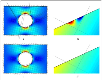
Fig. 8 Displacements and von-Mises stresses from numerical solutions with and without basis removal in the Neumann problem usingC1_Q2_{-splines and mesh size}_h₌₀_._{1. In the detailed view we note poor quality}

of the stresses on the boundary in the standard solution which is remedied when removing the problematic basis function.aStandard solution.bDetail in standard solution.cBasis removal solution.dDetail in basis removal solution

a b

Fig. 9 Example of numerical solution usingC1Q2splines and mesh sizeh=0.1. The mesh is rotatedπ/7 radians to induce cut situations and the removed basis functions are selected using the tolerance tol=0.01h2×√E.aMesh and removed spline basis functions.bNumerical solution

(18)

a b

Fig. 10 Convergence in||| · |||_hnorm and condition numbers for the manufactured problem using basis removal withC1Q2-spline basis. The tolerances used in the selection procedure istol=chp×√Eand we note that the choicesc=10−1andc=10−2give no visible diﬀerence in the error compared to using the full approximation space (c=0).aEnergy norm convergence.bCondition number

Conclusion

We have shown that:

• Basis function removal can be done in a rigorous way which guarantees optimal order of convergence and that the resulting linear system is not arbitrarily close to singular. These results critically depend on the smoothness of the B-spline spaces.

• Basis function removal is easy to implement and efficient since there is no fill-in in the stiffness matrix as is the case in for instance face based stabilization. Furthermore, basis function removal is consistent in contrast to the finite cell method.

We note however that even though the stiﬀness matrix is not arbitrarily close to singular the resulting condition number will in general be worse thanO(h−2_{), which is the optimal} scaling for standard ﬁnite element approximation of second order elliptic problems and therefore a direct solver or preconditioning in combination with an iterative solver is necessary in practice.

Authors’ contributions

All authors have prepared the manuscript. All authors read and approved the ﬁnal manuscript.

Competing interests

The authors declare that they have no competing interests.

Availability of data and materials

Not applicable.

Consent for publication

Not applicable.

Ethics approval and consent to participate

Not applicable.

Funding

(19)

Publisher’s Note

Springer Nature remains neutral with regard to jurisdictional claims in published maps and institutional aﬃliations.

Received: 11 January 2018 Accepted: 25 February 2018

References

1. Badia S, Verdugo F, Martín AF. The aggregated unﬁtted ﬁnite element method for elliptic problems. Sept: ArXiv e-prints; 2017.

2. Bazilevs Y, Beirão da Veiga L, Cottrell JA, Hughes TJR, Sangalli G. Isogeometric analysis: approximation, stability and error estimates forh-reﬁned meshes. Math Models Methods Appl Sci. 2006;16(7):1031–90.

3. Burman E. Ghost penalty. C R Math Acad Sci Paris. 2010;348(21–22):1217–20.

4. Burman E, Claus S, Hansbo P, Larson MG, Massing A. CutFEM: discretizing geometry and partial diﬀerential equations. Int J Numer Methods Eng. 2015;104(7):472–501.

5. Burman E, Hansbo P, Larson MG. A cut ﬁnite element method with boundary value correction. Math Comput. 2018;87:633–57.

6. Cottrell JA, Hughes TJR, Bazilevs Y. Isogeometric anlysis: toward integration of CAD and FEA. Chichester: John Wiley & Sons, Ltd.; 2009.

7. Dauge M, Düster A, Rank E. Theoretical and numerical investigation of the ﬁnite cell method. J Sci Comput. 2015;65(3):1039–64.

8. Embar A, Dolbow J, Harari I. Imposing Dirichlet boundary conditions with Nitsche’s method and spline-based ﬁnite elements. Int J Numer Methods Eng. 2010;83(7):877–98.

9. Folland GB. Introduction to partial diﬀerential equations. 2nd ed. Princeton: Princeton University Press; 1995. 10. Hansbo P, Larson MG, Larsson K. Cut ﬁnite element methods for linear elasticity problems. In: Bordas S, Burman E,

Larson M, Olshanskii M, (eds), In: Proceedings of the UCL Workshop 2016: geometrically unﬁtted ﬁnite element methods and applications. Berlin: Springer; 2018. To be published.

11. Johansson A, Larson MG. A high order discontinuous Galerkin Nitsche method for elliptic problems with ﬁctitious boundary. Numer Math. 2013;123(4):607–28.