The Thirty-Third AAAI Conference on Artificial Intelligence (AAAI-19)
Dynamic Spatial-Temporal Graph Convolutional Neural Networks for
Traffic Forecasting
Zulong Diao,
1Xin Wang,
2Dafang Zhang,
1∗Yingru Liu,
2Kun Xie,
1Shaoyao He
3 1The College of Computer Science and Electronic Engineering, Hunan University, Changsha 410082, China 2The Department of Electrical and Computer Engineering, Stony Brook University, Stony Brook, NY, 117943The College of Architecture, Hunan University, Changsha 410082
{zldiao, dfzhang, xiekun}@hnu.edu.cn,{x.wang, yingru.liu}@stonybrook.edu, [email protected]
Abstract
Graph convolutional neural networks (GCNN) have become an increasingly active field of research. It models the spatial dependencies of nodes in a graph with a pre-defined Lapla-cian matrix based on node distances. However, in many appli-cation scenarios, spatial dependencies change over time, and the use of fixed Laplacian matrix cannot capture the change. To track the spatial dependencies among traffic data, we pro-pose a dynamic spatio-temporal GCNN for accurate traffic forecasting. The core of our deep learning framework is the finding of the change of Laplacian matrix with a dynamic Laplacian matrix estimator. To enable timely learning with a low complexity, we creatively incorporate tensor decom-position into the deep learning framework, where real-time traffic data are decomposed into a global component that is stable and depends on long-term temporal-spatial traffic rela-tionship and a local component that captures the traffic fluc-tuations. We propose a novel design to estimate the dynamic Laplacian matrix of the graph with above two components based on our theoretical derivation, and introduce our design basis. The forecasting performance is evaluated with two real-time traffic datasets. Experiment results demonstrate that our network can achieve up to25%accuracy improvement.
Introduction
Traffic forecasting is fundamental to the performance of many components in intelligent transportation systems (ITS). The accurate and reliable traffic forecasting can as-sist in proactive and dynamic traffic control as well as in-telligent route guidance, which will help alleviate the huge congestion problem in the system. In this paper, we are in-terested in simultaneously predicting the traffic of multiple road segments in a road network.
Great efforts have been devoted to improve the traffic forecasting accuracy (Diao et al. 2018). Some studies ap-ply traditional machine learning methods, such as auto-regressive and moving average model (ARMA) (Williams and Hoel 2003) and support vector regression (SVR) (Chen et al. 2015) and etc, to forecast future traffic. As most of these methods are linear and not suitable for handling
∗
Corresponding author
Copyright c⃝2019, Association for the Advancement of Artificial Intelligence (www.aaai.org). All rights reserved.
volatile traffic data, the forecasting accuracy is often low. In recent years, the prediction methods based on deep learn-ing have received considerable attention. Some attempts have been made to apply deep Recurrent Neural Networks (RNN)(Wu and Tan 2016) and Convolution Neural Network (CNN) (Zhang et al. 2016; Zhang, Zheng, and Qi 2016; Ma et al. 2017) to predict traffic flow. However, these meth-ods are not suitable to apply to the data points with ir-regular graph relationship. As graph structure arises natu-rally in the traffic network, Graph Convolutional Neural Net-work (GCNN) is the appealing choice (Yu, Yin, and Zhu 2017a). GCNN with deep architectures have proven to be very efficient in short-term traffic forecasting area (Yao et al. 2018). By incorporating the spectral graph theory (Fan 1997), GCNN is efficient in handling signals that live on irregular or non-Euclidean domains. Nevertheless, existing GCNN frameworks have some limitations that make them less efficient in traffic forecasting.
GCNN heavily depend on the Laplacian matrix of a graph, which is defined as the difference between the diagonal ma-trix of node degrees and the adjacency mama-trix. Previous GCNN studies rely on the key assumption that the Lapla-cian matrix is strictly unchanged and available (i,e. the ad-jacency matrix of the input graph is constant). However, our previous studies demonstrate that there are huge differences between traffic patterns during different time spans. In addi-tion, traffic accidents may occur every day, which will also affect the relationship between road segments in the road network. These factors will lead to the dynamic changes of adjacency matrix thus the Laplacian matrix. Therefore, the exact Laplacian matrix of the graph could be time-variant and generally intractable.
To address the issues above, we propose a novel spatial-temporal structure to more accurately forecast network-wide traffic speed, and we call it dynamic GCNN (DGCNN). Compared with existing GCNN-based methods, our paper makes the following contributions:
one determined by the road network structure and the local one determined by specific time-of-day or traffic events. We pre-train our tenor decomposition layer with a particular loss function.
• To learn the Laplacian matrix at a specific time-of-day dy-namically according to the global and local data compo-nents, we design a deep learning-based Laplacian matrix estimator with detailed theoretical derivation and design basis. The Laplacian matrix estimated in real-time will be sent to the graph convolutional layers for forecasting.
The rest of this paper is organized as follows. We first sum-marize the related work of GCNN in Section 2, and in-troduce the background knowledge in Section 3. We then present the technical details of our novel DGCNN model in Section4. After that, we evaluate the performance of our proposed model through experiments on real-world data sets in Section5, and conclude our work in Section6.
Related Works
In this section, we summarize the literature work and pro-vide the motivations of our work.
GCNN is extended from convolutional neural networks (CNN) with consideration of graph structures. Existing graph convolutional neural networks can be mainly divided into two categories according to the convolutional oper-ator. One is based on concepts from the vertex domain (Niepert, Ahmed, and Kutzkov 2016; Monti et al. 2017; Hechtlinger, Chakravarti, and Qin 2017; Puy, Kitic, and P´erez 2017); The other is based on concepts from the graph spectral domain. As we cannot express a meaningful trans-lation operator in the vertex domain (Defferrard, Bresson, and Vandergheynst 2016), we prefer defining the convolu-tion operator in the spectral domain in this paper.
Spectral graph theory enables us to extend many of the important mathematical ideas and intuitions from classical Fourier analysis to the graph setting. In recent years, GCNN and its variants have been applied to various areas, such as image classification and task forecasting (Bruna et al. 2013; Yu, Yin, and Zhu 2017b; Shuman et al. 2013; Henaff, Bruna, and LeCun 2015; Defferrard, Bresson, and Vandergheynst 2016; Kipf and Welling 2016; Yu, Yin, and Zhu 2017a; Srivastava, Greff, and Schmidhuber 2015).
Previous studies on traffic forecasting with GCNN (Yu, Yin, and Zhu 2017a; Yao et al. 2018; Puy, Kitic, and P´erez 2017) have a fatal drawback. They seldom consider the change of spatial dependencies with the gradual structural evolution of the road network. The Laplacian matrix rep-resents spatial dependencies between road segments. As shown in Section3, GCNN heavily depends on the Lapla-cian matrix L. Keeping the same Laplacian matrix all the time may lead to a significant performance decrease. Yao et al. (Yao et al. 2018) apply the traffic flow data of road seg-ments to model dynamic spatial dependencies between road intersections. However, this method increases the burden of data collection and still doesn’t track the dynamic change of the Laplacian matrix.
To satisfy the forecasting requirements under a dynamic network structure, we propose a dynamic spatio-temporal
graph convolutional neural network. Our framework will automatically modify the Laplacian matrix according to changes of spatial dependencies hidden in the traffic data.
Preliminary
Before presenting our detailed design of the spatial-temporal framework, we provide some background knowledge in this paper. Graph CNN helps us make traffic forecasting with consideration of graph structures in the road network. Based on the Equation 5 in the area of signal processing, we pro-pose a deep learning method to learn the Laplacian ma-trix. We incorporate tensor operations into our deep learn-ing framework to extract the long-term and short-term traffic tensor from the real-time tensor.
Graph CNNs
Given a directed graphG= (ν, ε, W), where the setν con-tains|ν|=pvertices;εrepresents a set of edges,Wdenotes the weight matrix ofG. A signalx:ν →Rdefined on the nodes of the graph may be represented as a vectorx∈Rp,
wherexi is the signal value at the ith node. We have the
graph LaplacianL=D−W and the eigen decomposition ofL =UΛUT, where D is a diagonal matrix with thei
th
element of the diagonal line being the degree of the nodei: Dii=∑jWij andU is an orthogonal matrix.
The Fourier transform for x is defined as xˆ = UTx. Hence, the graph convolution of x and y defined in the Fourier domain is
x∗Gy=U((UTx)
⨀
(UTy)), (1)
where⨀
is the element-wise Hadamard product. It follows that a signalxis filtered bygθas
y=gθ(L)x=gθ(UΛUT)x=U gθ(Λ)UTx. (2)
To make the filterK-localized in space and reduce its com-putational complexity, Eq. (2) can be further defined as
y=U gθ(Λ)UTx=U( K−1
∑
k=0
θkΛk)UTx= K−1
∑
k=0
θkLkx.
(3) where the parameter θ ∈ RK is a vector of polynomial
Fourier coefficients. This filter restricts the hop distance dg(i, j)between two nodesiandjto be withinKhops, that
isLKi,j = 0whendg(i, j)≥K. Consequently, spectral
fil-ters represented byKth-order polynomials of the Laplacian
are exactly K-localized.
A signal on graphGofpnodes can be described as a ma-trixXconsisting ofcinvectors of sizep. Consequently, for
the signalX = [x1, x2,· · ·, xcin], a 1-D graph convolution
operation with a kernel tensorθof size(cin, cout, K)is
yj=
∑
i∈[1,cin],k∈[1,K]
θijkLkxi, j= 1,2, ..., cout (4)
wherecin andcout represent the size of the input feature
Graph Signal Processing
In the area of signal processing on graphs, signals are mod-eled as functions on the vertices of a weighted graph. A major challenge in this field is that of learning the graph structure from data. The learned graph must have a meaning-ful interpretation and be usemeaning-ful for analysis. Given a set of nodesV and a set of corresponding signals on those nodes, the graph structure is learnt by estimating a matrixLwhose nonzero patterns define the edge connectivity of the graph.
Given ap-dimensional random graph signalxand its N observations x1,· · ·,xN, its sample covariance is Q =
1
N
∑N
i=1xix
T
i. It’s often formulated as a matrix optimiza-tion problem and focus on an efficient algorithmic soluoptimiza-tion. According to the maximum likelihood estimate of L, we have (Pavez and Ortega 2016)
min
L≽0;Lij60,∀i̸=j;−logdet(L) +tr(QL) (5)
Minimizingtr(QL)is equivalent to promoting the average smoothness. The log det function acts as a barrier on the minimum eigenvalue ofL, thus enforcing the positive semi-definite constraint. The sign constraints can be handled using Lagrange multipliers.
Tensor Operations
Tensor operations are widely used in various applications (Xie et al. 2018; Xie et al. 2017), such as traffic prediction and anomaly detection.
Tensor Unfolding: For an N-way tensorχ∈RI1×···×IN,
its mode-n unfolding χ[n] ∈RIn×(In+1In+2···INI1I2···In−1)
contains the tensor elementai1,i2,···,iN at the position in the
unfolding matrix with its row index in and column index
equal to∑N
k=1,k̸=nik×∏ N
m=k+1,m̸=nIm.
n-mode product: Then-mode product of anN-way
ten-sorχ∈RI1×···In···×IN with matrixU ∈
RJ×Inproduces a
tensor with size(I1× · · · ×In−1×J×In+1× · · · ×IN)
and defined as
(χ×nU)i1···in−1jin+1···iN =
In
∑
in=1
xi1i2···iNUjin (6)
where×nis the n-mode product operation.
Tucker decomposition: Given a tensorχ∈RI1×···×IN,
we can decompose it into a low rank core G ∈
Rr1×r2×···×rN by projecting along each of its modes with
projection factors(U1,· · · , UN), withUk ∈ Rrk×Ik, k ∈ (1,· · ·, N). We can write as:
χ=G×1U1×2U2× · · · ×N UN (7)
whererk represents the selected rank in mode-kof the
ten-sorχ.
Problem and Model
In this section, we introduce the problem of network-wide traffic forecasting, and the basic framework of our proposed system.
We are interested in simultaneously forecasting the traffic speed of multiple road segments. We define a road network as a directed graphG= (ν,ε, W), whereνis a set of ver-tices each corresponding to a road segment,εrepresents a set of edges with each edge connected between two road segments in the network, W denotes the adjacency matrix ofG. The average traffic speed of the road segmentiin the time intervaltis represented byvi(t).
DST-Conv Block
DST-Conv Block
Output Layer
Temporal Conv
Spatial Graph-Conv
Temporal Conv
2-D Conv
L
ap
la
ci
an
M
at
rix
E
st
im
at
o
r
GLU
A B C
m p R
X
1 p R Y
L
L
DST-Conv Block
Temporal Conv
L
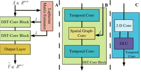
Figure 1: The framework of DGCNN
Given historical speed observations of proad segments
{vi(·)} p
i=1 at time (t−m+ 1,· · · , t−1, t), our task is to
predict the value of{vi(t+ ∆))} p
i=1, where∆denotes the
prediction horizon. If we put the historical data together, we can get a data matrixX.
X = ⎡
⎢ ⎣
v1(t−m+ 1) v1(t−m+ 2) · · · v1(t)
v2(t−m+ 1) v2(t−m+ 2) · · · v2(t)
· · · ·
vp(t−m+ 1) vp(t−m+ 2) · · · vp(t)
⎤
⎥ ⎦
(8)
As shown in Figure 1 A, our deep learning framework is composed of three modules: a Laplacian matrix estima-tor, two spatial-temporal convolutional blocks and an output layer. Each spatial-temporal convolutional block is formed as a “sandwich” structure as in Figure 1 B with two gated temporal convolutional layers and a spatial graph convolu-tional layer in between. So we can take full advantage of spatial dependencies and temporal dependencies hidden in traffic data to assist our forecasting task. The downscaling of channels in the spatial graph convolution layer can also help reduce the number of parameters and the time consumption in training. The output layer contains a temporal convolu-tional layer and a fully connected layer which transforms the size of the temporal dimension to1and generate the fi-nal output (Rp×1). As the focus of this paper, the Laplacian
Compared with RNN-based models with an iterative op-eration over each time slot, CNN-based models process a block of data together and have the superiority of fast train-ing and simple structures. Therefore we employ entire con-volutional structures on time axis for a window of data to capture dynamic temporal behavior of traffic flows. Next we will give a detailed description of the Laplacian matrix esti-mator and the spatial-temporal convolutional block.
Dynamic Spatial-Temporal Graph
Convolutional Neural Network
The Laplacian matrix is crucial for determining the recep-tive field of the graph convolutional operation. An inaccurate Laplacian matrix will reduce the forecasting accuracy. For a graph withNnodes, the Laplacian matrix hasN×Nentries. Obtaining accurate Laplacian matrix in real-time faces two major challenges. First, the number of parameters to learn for the complete matrix will increase quickly with the net-work size. Second, the traditional convergent gradient de-scent algorithm is time consuming and cannot update the Laplacian matrix quickly upon the arrival of new traffic data to meet the need of online traffic forecasting.
We first present our design of a dynamic Laplacian matrix estimator, and then propose a novel spatial-temporal convo-lutional neural network for efficient traffic prediction.
Dynamic Laplacian Matrix Estimator
Given a global Laplacian matrix that represents the static graph structure of a traffic network, the real-time Laplacian matrix will fluctuate up and down around it. The perturba-tion is the result of minor changes of the graph structure, which is mainly caused by short-term traffic pattern and ac-cidents. Thus we only need to determine the variation of Laplacian matrix based on the short-term traffic. As a result of spatial and temporal correlation, long-term traffic data form a low rank tensor. Because the traffic dynamics and abnormality are rare in the temporal dimension, short-term data form a sparse tensor in the temporal dimension.
We thus incorporate the tensor operation into the neural network and decompose the traffic tensor into two compo-nents, a low-rank tensor that maintains the long-term and highly correlated traffic information, and a sparse tensor that tracks the dynamic changes of traffic. Accordingly, our Laplacian matrix estimator includes two parts, a Tensor De-composition Layer (TDL) and a unit for dynamic Laplacian matrix learning.
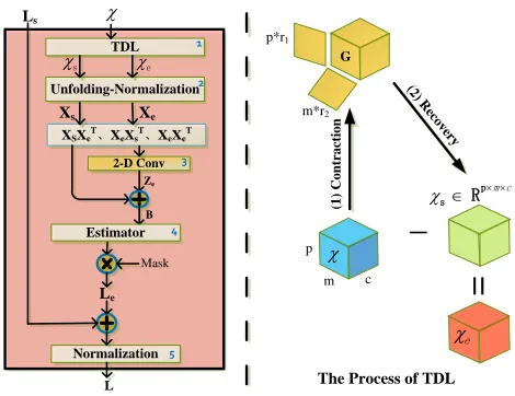
Tensor Decomposition Layer In our Laplacian matrix
es-timator, we apply TDL to extract the global and local com-ponent of the traffic data with two operations, contraction and recovery. On the right part of Figure 2, we show a 3-order traffic tensor χ with (p, m, c) corresponding to the number of nodes in the spatial domain, number of time slots to consider in the temporal domain and the number of chan-nels thus states to monitor. We setcto1in this paper to fo-cus on the monitoring of traffic speed.(r1, r2)corresponds
to the rank of the spatial and temporal modes, and will be generally lower thanpandmdue to the traffic correlation in spatial and temporal domains.
Ls
Mask TDL
Le
Normalization
L
G
p
m c m*r2
p*r1
_
=
Unfolding-Normalization
XSXeT、XeXsT、XeXeT
2-D Conv
Xs Xe
B Ze
Estimator
1
2
3
4
5
c
m
p
s R
(1
)
C
o
n
tr
a
ct
io
n
(2 ) R
ecov ery
e
The Process of TDL s
e
Figure 2: Laplacian Matrix Estimator
In the contraction operation, TDL runs twon-mode prod-ucts along the spatial and temporal modes with the projec-tion factorsU1∈Rp×r1,U
2∈Rm×r2 to projectχinto the low-dimensional space:
χ=G×1U1×2U2. (9)
Given χ, U1 and U2, we can easily calculate the
low-dimensional tensor G according to the Equation 9. In the recovery operation, TDL estimates the low-rank tensorχs through the expansion from the low dimensional space:
χs=G×1U1×2U2×2U2T ×1U
T
1 (10)
The projection factorsU1 andU2are set as the
parame-ters to learn through gradient back-propagation in our deep learning framework. Once the training process is completed, the two projection factors can be applied to estimate the long-term trafficχs and used in each time slot, so we can obtain the short-term dynamic traffic tensorχeas follows:
χe=χ−χs. (11)
Learning of Dynamic Laplacian Matrix The
approxi-mated low-rank tensor χs is impacted by the long-term and global dependencies in spatial and temporal dimensions. The sparse tensorχerepresents the local fluctuation within a specific time span of a day, which is affected by short-term spatial and temporal dependencies as well as external factors such as traffic accidents and weather.
We define the dynamic Laplacian matrix at any time as L=Ls+Le, whereLsandLerepresent the global
Lapla-cian matrix and the local LaplaLapla-cian matrix respectively.Le
acts as a short-term perturbation on L. We compute the global Laplacian matrix based on the distances among sen-sors employed on each road segment.
To find the detailed Laplacian matrix Le, we make the
elements being zero. According to the Karush-Kuhn-Tucker (KKT) conditions we have:
L= (Q+Z)−1
subject to Z =ZT, Zij >0
(12)
The matrix Z acts as a perturbation on the sample co-variance matrix Q such that the learned Laplacian matrix Z can represent the spatial dependencies of the road net-work. Through unfolding and zero-mean normalization, we can transfer the low-rank tensorχsand sparse tensorχeto two matricesXs ∈ Rp×(r2∗r3) andX
e ∈ Rp×(r2∗r3).X
s
can be considered as a low-rank matrix that corresponds to the long-term traffic data. Replacing the sample covariance matrix withXsXsT, based on Eq. 12, we have:
Ls= (XsXsT+Zs)
−1
(13)
Similarly, inserting the real-time Laplacian matrixL=Ls+
Leand its corresponding traffic dataX =Xs+Xeinto the
Eq. (12), then:
Ls+Le= [(Xs+Xe)(Xs+Xe) T
+Zs+Ze]
−1
= [(Xs+Xe)(XsT +XeT) +Zs+Ze]
−1
= [(XsXsT+Zs)+(XsXeT+XeXsT+XeXeT+Ze)]
−1
= [Ls−1+(XsXeT+XeXsT+XeXeT+Ze)]
−1
(14) whereLsrepresents the global Laplacian matrix andZs
rep-resents the corresponding Laplacian multipliers.
Eq. (13) and Eq. (14) give the global Laplacian matrixLs
and the dynamic Laplacian matrixLrespectively. Although Lsis given in advance, the complexity of finding the matrix
inversion isO(n3). To simplify the calculation, we would like to get rid of the inverse operations in Eq. (14), and then learnLebased on deep learning methods.
Based on (Henderson and Searle 1981), for two matrices AandBwithAandA+Binvertible, we have
(A+B)−1=A−1−A−1B(E+A−1B)−1A−1 (15)
Erepresent an identity matrix. LetBrepresent(XsXeT+
XeXsT+XeXeT+Ze), based on Eq. (15), the Eq. (14) can
be rewritten as:
Ls+Le=Ls−LsB(E+LsB)−1Ls
Le=−LsB(E+LsB)
−1
Ls (16)
Iteratively applying the Eq. (15) to expand(E+LsB)−1,
Eq. (16) can be further expanded as:
Le=
∝ ∑
i=1
(−1)iLs(BLs) i
(17)
We can estimateLe with a finite number of summation
operations:
Le= I
∑
i=1
(−1)iLs(BLs)i+o(BLs) (18)
whereo(BLs)is the error from Eq. 17.
The equation used to estimate Le doesn’t include
the inverse operations, which greatly reduces the time consumption of our deep learning framework. As XsXeT, XeXsT, XeXeT can be computed directly
with matrices Xs, Xe, we only need to learn Ze in B.
Ze∈Rp×p, wherepequals to the number of road segments on the road network. To avoid involving too many parame-ters in training and ensure the scalability of our model with the expansion of the road network, we employ two 2-D convolutional layers for the data fitting.
For the overall dynamic Laplacian matrix estimator shown on the left part of Figure 2, the input data will go through five sub-processes as follows:
1. Tensor Decomposition. The Tensor Decomposition
Layer (TDL) incorporates the tensor operations into the neural network and splits the traffic tensorχinto a low rank tensorχsand a sparse tensorχe.
2. Unfolding-Normalization. After an unfolding operation
along the spatial dimension and an zero-mean normaliza-tion, the two tensors generated by the first sub-process are further translated to two zero-mean matrices Xs, Xe ∈
Rp×(m∗c), based on which we can easily find the values ofXsXeT,XeXsT,XeXeT.
3. 2-D Conv. We stack two2-D convolutional layers to fit
the Lagrange multipliersZe. The input data of the first
convolutional layer is a 3-D tensor Rp×p×3, which is formed by stackingXsXeT,XeXsT,XeXeTtogether. The
size of the output feature maps on the two convolutional layers are set to3and1respectively.
4. Estimator. We find matricesB andLeaccording to the
Eq. (18).
5. Normalization. We findL=Ls+Leand then normalize
LthroughD−1/2LD−1/2, whereDis a diagonal matrix
with the element on a row equal to the absolute value of the summation ofL’s off-diagonal elements on that row.
Compared with most graph learning methods in the liter-ature, our deep learning framework has higher execution ef-ficiency. Without the inverse operation, our estimator won’t increase the burden of the deep learning framework when performing traffic forecasting.
Pre-training the TDL Before training the whole deep
learning framework, we pre-train TDL to initialize its pa-rameters. The corresponding loss function is
L(U1, U2) =
ξ
∑
tr(XsLsXsT) +β∥Xe∥F. (19)
where U1, U2 are trainable parameters in TDL, Ls is the
global Laplacian matrix given in advance.ξrepresents the total number of data samples for training.tr is a trace op-eration. Xs is the matrix extracted from the traffic
com-ponent χs by TDL, and β is a weight coefficient which
controls the proportion of two items in Eq. (19). Minimiz-ing tr(XsXsTLs) is equivalent to promoting the average
Ls withXs and guarantees thatXsextracted by TDL can
meet the Eq. (13).
Spatial-Temporal Convolutional Block
In our learning framework, we apply a spatio-temporal con-volutional block to jointly process graph-structured time se-ries and fuse features from both temporal and spatial do-mains.
Gated CNNs for Extracting Temporal Features We set
a 2-D temporal convolutional layer to capture short-term temporal features of traffic flows. Given the input of tem-poral convolutional layer χ ∈ Rp×m×cin, where p, m,
cin represent the size of the spatial, temporal and
chan-nel dimensions respectively, the convolutional kerchan-nel Γ ∈
R1×K×cin×2cout will map the input to an output element [Y1, Y2] ∈ Rp×(m−K+1)×(2cout) (Y
1, Y2 are split into half
with the same size of channels). As shown in Figure 1 C, the temporal gated convolution can be defined as:
Γ∗τχ=Y1
⨀
σ(Y2) (20)
whereY1, Y2 ∈ Rp×(m−K+1)×cout are the input of gates in gated linear units (GLU) separately, and⨀
denotes the element-wise Hadamard product. The sigmoid gate σ(Y2)
controls which inputsY1of the current status are relevant for
discovering compositional structure and dynamic variances in time series.
Graph CNNs for Extracting Spatial Features Given the
input of graph convolutional layer asχ∈Rp×m×cin, where
p,m,cirepresent the size of the spatial, temporal and
chan-nel dimensions respectively. We split the input data intom parts along the temporal dimension, with each being a ma-trixRp×cin, and then capture spatial features of each part by
a1-D graph convolutional layer. In order to speed up the1 -D graph convolutional operation, we employ the Chebyshev polynomialTk(x)to approximate kernels (Yu, Yin, and Zhu
2017a). The graph convolution in Eq. (4) can then be rewrit-ten as:
yj =
∑
i∈[1,cin],k∈[1,Ks]
θijkTk( ˜L)xi, j= 1,2, ..., cout (21)
whereyj ∈Rp×cout.T
k( ˜L)is the Chebyshev polynomial of
orderkevaluated at the scaled LaplacianL˜= 2L/λmax−In.
Experiments
Experimental Settings
Data. We evaluate the performance of our proposed model
using two real-world large-scale datasets collected from the monitoring of traffic in New York City (NYC) and in Cali-fornia, respectively:
• NYC: This traffic dataset contains traffic information col-lected from traffic speed detectors deployed on road seg-ments of Manhattan district in New York city. We select 50sensors and collect2months of data ranging from De-cember1st2017to January30th2018.
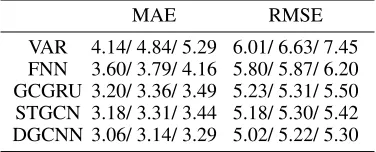
Table 1: Forecasting error given by MAE and RMSE on NYC dataset (15/30/45 min)
MAE RMSE
VAR 4.14/ 4.84/ 5.29 6.01/ 6.63/ 7.45 FNN 3.60/ 3.79/ 4.16 5.80/ 5.87/ 6.20 GCGRU 3.20/ 3.36/ 3.49 5.23/ 5.31/ 5.50 STGCN 3.18/ 3.31/ 3.44 5.18/ 5.30/ 5.42 DGCNN 3.06/ 3.14/ 3.29 5.02/ 5.22/ 5.30
• PeMS: This traffic dataset contains real-time speed data from freeways in California. We select 50/142/228 de-tectors and collect 6 months of data range from April 1st2017to September30th2017.
The traffic data are aggregated and output by each detec-tor every 5 minutes. All studies use one hour as the hisdetec-tori- histori-cal time window to forecast the traffic condition in the next 15/30/45 minutes according to 12observed data points in the window.
Evaluation Metric and Baselines. We adopt Mean
Aver-age Error (MAE) and Rooted Mean Square Error (RMSE) to evaluate the performance of different methods. We also implement four baseline schemes for the performance ref-erence: 1. Vector Autoregression (VAR); 2) Feed-Forward Neural Network (FNN); 3) Graph Convolutional GRU (GC-GRU, published in ICLR-2018) (Li et al. 2017); and 4) Spatio-Temporal Graph Convolutional Networks (STGCN, published in IJCAI-2018) (Yu, Yin, and Zhu 2017a).
All these deep learning models are trained for50epochs with batch size as50. The initial learning rate is10−3with a
decay rate of0.7after every5epochs. Both the graph convo-lution kernel size and temporal convoconvo-lution kernel size are set to 3. The size of the output feature map in the spatial-temporal convolution block of DGCNN are 64,16,64 re-spectively.
Performance Comparison
2 4 6 8 10 12 14 16 Parameter I
4.04.2 4.4 4.6 4.8 5.05.2 5.4
Test MAE
0 10 20 30 40 50
Training Epoch 4
5 6 7 8 9
GCGRU STGCN DGCNN
Figure 3: Test MAE versus the parameter I in DGCNN (left); Test MAE versus the number of training epochs (right). (PeMS-50)
Parameter Selection and Training Efficiency In order to
Laplace matrix. When the parameterIis greater than6, the rate of decline tends to be slow. Therefore, we set the param-eterIto6in this paper.
15 30 45
minutes ahead 3
4 5 6 7 8
Test MAE
(a) PeMS-50
5 4 3 2 1
15 30 45
minutes ahead 3
45 6 7 8
(b) PeMS-142
15 30 45
minutes ahead 3
45 67 8
(c) PeMS-228
Figure 4: Forecasting accuracy: 1) DGCNN, 2) STGCN, 3) GCGRU, 4) FNN, 5) VAR.
Forecasting Accuracy We run each model10times and
report the average results. From Table 1 and Figure 4, our proposed DGCNN outperforms all competing baselines by achieving the lowest RMSE and MAE on both datasets for the traffic forecasting.
In brief, the traditional linear prediction method VAR per-forms the worst due to its incapability of handling volatile traffic data. Compared with other three deep learning mod-els, our DGCNN also perform better with on average8%−
10%accuracy improvement. Traffic patterns and spatial de-pendencies on road network are dynamic. Overlooking the dynamic changes of spatial dependencies on the road net-work, the forecasting error of reference schemes are higher.
0.1 0.2 0.3 0.4 0.5 0.6 0.7 0.8 0.9 1.0
4 5 6 7 8 9 10
Test MAE
3 2 1
0.1 0.2 0.3 0.4 0.5 0.6 0.7 0.8 0.9 1.0
45 6 7 8 9 10
3 2 1
0.1 0.2 0.3 0.4 0.5 0.6 0.7 0.8 0.9 1.0
45 67 8 9 10
3 2 1
0.1 0.2 0.3 0.4 0.5 0.6 0.7 0.8 0.9 1.0Fault-Ratio
4 5 6 7 8 9 10
Test MAE
(a) PeMS-50
3 2 1
0.1 0.2 0.3 0.4 0.5 0.6 0.7 0.8 0.9 1.0Fault-Ratio
45 6 7 8 9 10
(b) PeMS-142
3 2 1
0.1 0.2 0.3 0.4 0.5 0.6 0.7 0.8 0.9 1.0Fault-Ratio
45 67 8 9 10
(c) PeMS-228
3 2 1
Figure 5: Fault-tolerance comparison with state-of-the-art models based on graph CNNs: 1) DGCNN, 2) STGCN (IJCAI-2018), 3) GCGRU (ICLR-2018).
Fault Tolerance Comparison The real-time traffic
sam-ples may be partial abnormal as a result of sensor malfunc-tion or traffic accidents on some road segments. To examine
the fault-tolerance ability in extreme environments, we ran-domly select a fraction (10%to100%) of road segments to sabotage their12historical observations. We carry out two groups of studies and forecast the traffic condition in the next 45minutes: On the top row of Figure 5, the damaged ob-servations from nodes selected are replaced with zero-mean white Gaussian noise (variances 1.0). On the bottom row, zeros are used to replace the “damaged” observations.
Fusing the spatial-temporal information with dynamic Laplacian matrix, our model is shown to be more fault tol-erant with on average10%−25%accuracy improvement compared with two state-of-the-art models based on graph CNNs. Even when the fault ratio reaches0.9, DGCNN still has a strong forecast capability. With the same amount of noise contamination, other models’ performance drops dra-matically without exception. Comparing the results over three PeMS datasets, the performance gain of our model will become larger with the increase of road network scale. Our DGCNN model can detect the changes of spatial de-pendencies hidden in “contaminated” traffic samples and ad-just the receptive field of graph convolution operations. The right of Figure 3 shows the learning curves of three mod-els with roughly the same number of parameters. With the increase of training epochs, DGCNN achieves the lowest validation error compared with GCNN and STGCN, which shows its training effectiveness. The intuition is that the dy-namic Laplacian matrix estimator gives the model the ability and flexibility to capture the influence from various factors in the road network.
0
10
20
30
40
(a) 17/12/25 07:00-09:30
0
10
20
30
40
Loc1
Loc2
0
10
20
30
40
(b) 17/12/25 09:30-14:00
0
10
20
30
40
Loc1
Loc2
1.0
0.8
0.6
0.4
0.2
0.0
Figure 6: Spatial dependencies learning on two consecutive time spans.
Spatial Dependencies Learning To identify the
Laplacian matrix. The two locations marked with “LOC1” and “LOC2” also demonstrate that our model can learn the local changes of the Laplacian matrix.
Conclusion and Future Work
In this paper, we propose a novel dynamic graph convolution neural network (DGCNN) for traffic forecasting. To the best of our knowledge, this is the first graph convolution neural network that can follow the evolution of spatial dependen-cies. The experiment results demonstrate that our proposed neural network can achieve on average10%−25%higher accuracy compared to other models. The proposed dynamic Laplacian matrix estimator plays an important role in the forecasting process. In the future work, we also plan to com-bine our DGCNN with other deep learning methods to learn the structured features hidden in the input data.
Acknowledgments
The work is supported by the National Natural Sci-ence Foundation of China under Grant No.61472130 and No.61572184, a Planned Science and Technology Project of Hunan Province in 2017, the NSF grant CNS-1526843 and ECCS-1731238, a Hunan Provincial Natural Science Foun-dation of China under Grant No.2017JJ1010.
References
Bruna, J.; Zaremba, W.; Szlam, A.; and Lecun, Y. 2013. Spectral networks and locally connected networks on graphs. Computer Science.
Chen, R.; Liang, C. Y.; Hong, W. C.; and Gu, D. X. 2015. Fore-casting holiday daily tourist flow based on seasonal support vector regression with adaptive genetic algorithm. Applied Soft Comput-ing26(C):435–443.
Cui, Z.; Ke, R.; and Wang, Y. 2018. Deep bidirectional and uni-directional lstm recurrent neural network for network-wide traffic speed prediction.
Defferrard, M.; Bresson, X.; and Vandergheynst, P. 2016. Con-volutional neural networks on graphs with fast localized spectral filtering.
Diao, Z.; Zhang, D.; Wang, X.; Xie, K.; He, S.; Lu, X.; and Li, Y. 2018. A hybrid model for short-term traffic volume prediction in massive transportation systems. IEEE Transactions on Intelligent Transportation Systems(99):1–12.
Fan, R. K. C. 1997. Spectral graph theory. Published for the Conference Board of the mathematical sciences by the American Mathematical Society,.
Hechtlinger, Y.; Chakravarti, P.; and Qin, J. 2017. A generalization of convolutional neural networks to graph-structured data. Henaff, M.; Bruna, J.; and LeCun, Y. 2015. Deep convolutional networks on graph-structured data.CoRRabs/1506.05163. Henderson, H. V., and Searle, S. R. 1981. On deriving the inverse of a sum of matrices.Siam Review23(1):53–60.
Kipf, T. N., and Welling, M. 2016. Semi-supervised classification with graph convolutional networks.
Li, Y.; Yu, R.; Shahabi, C.; and Liu, Y. 2017. Diffusion convolu-tional recurrent neural network: Data-driven traffic forecasting. Ma, X.; Dai, Z.; He, Z.; Ma, J.; Wang, Y.; and Wang, Y. 2017. Learning traffic as images: A deep convolutional neural network
for large-scale transportation network speed prediction. Sensors
17(4).
Monti, F.; Boscaini, D.; Masci, J.; Rodola, E.; Svoboda, J.; and Bronstein, M. M. 2017. Geometric deep learning on graphs and manifolds using mixture model cnns. 5425–5434.
Niepert, M.; Ahmed, M.; and Kutzkov, K. 2016. Learning convo-lutional neural networks for graphs. 2014–2023.
Pavez, E., and Ortega, A. 2016. Generalized laplacian precision matrix estimation for graph signal processing. InIEEE Interna-tional Conference on Acoustics, Speech and Signal Processing. Puy, G.; Kitic, S.; and P´erez, P. 2017. Unifying local and non-local signal processing with graph cnns.
Shuman, D. I.; Narang, S. K.; Frossard, P.; Ortega, A.; and Van-dergheynst, P. 2013. The emerging field of signal processing on graphs: Extending high-dimensional data analysis to networks and other irregular domains. IEEE Signal Processing Magazine
30(3):83–98.
Srivastava, R. K.; Greff, K.; and Schmidhuber, J. 2015. Highway networks.Computer Science.
Williams, B. M., and Hoel, L. A. 2003. Modeling and forecast-ing vehicular traffic flow as a seasonal arima process: Theoretical basis and empirical results.Journal of Transportation Engineering
129(6):664–672.
Wu, Y., and Tan, H. 2016. Short-term traffic flow forecasting with spatial-temporal correlation in a hybrid deep learning framework. Xie, K.; Li, X.; Wang, X.; Xie, G.; Wen, J.; Cao, J.; and Zhang, D. 2017. Fast tensor factorization for accurate internet anomaly de-tection.IEEE/ACM transactions on networking25(6):3794–3807. Xie, K.; Li, X.; Wang, X.; Xie, G.; Wen, J.; and Zhang, D. 2018. Graph based tensor recovery for accurate internet anomaly detec-tion. In IEEE INFOCOM 2018-IEEE Conference on Computer Communications, 1502–1510. IEEE.
Yao, H.; Tang, X.; Wei, H.; Zheng, G.; Yu, Y.; and Li, Z. 2018. Modeling spatial-temporal dynamics for traffic prediction. Yu, B.; Yin, H.; and Zhu, Z. 2017a. Spatio-temporal graph convolu-tional networks: A deep learning framework for traffic forecasting. Yu, B.; Yin, H.; and Zhu, Z. 2017b. Spatio-temporal graph con-volutional neural network: A deep learning framework for traffic forecasting.CoRRabs/1709.04875.
Zhang, J.; Zheng, Y.; Qi, D.; Li, R.; and Yi, X. 2016. Dnn-based prediction model for spatio-temporal data. InACM Sigspatial In-ternational Conference on Advances in Geographic Information Systems, 92.