www.adv-radio-sci.net/8/211/2010/ doi:10.5194/ars-8-211-2010
© Author(s) 2010. CC Attribution 3.0 License.
Radio Science
Simplified modeling of EM field coupling to complex cable bundles
B. Schetelig1, J. Keghie1, R. Kanyou Nana1, L.-O. Fichte1, S. Potthast2, and S. Dickmann1
1Faculty of Electrical Engineering, Helmut-Schmidt-University/University of the Federal Armed Forces Hamburg, Germany 2Bundeswehr Research Institute for Protective Technologies and NBC Protection (WIS), Munster, Germany
Abstract. In this contribution, the procedure “Equivalent Cable Bundle Method” is used for the simplification of large cable bundles, and it is extended to the application on dif-ferential signal lines. The main focus is on the reduction of twisted-pair cables. Furthermore, the process presented here allows to take into account cables with wires that are situ-ated quite close to each other. The procedure is based on a new approach to calculate the geometry of the simplified ca-ble and uses the fact that the line parameters do not uniquely correspond to a certain geometry. For this reason, an opti-mization algorithm is applied.
1 Introduction
To assure the immunity of cable-wired communication sys-tems to external electromagnetic influences, one needs to know the disturbances coupled into the connecting cables to carry out an evaluation at the inputs of the connected de-vices based on its prescriptive limits. From several research projects, it is known that coupling via the cables is often quite important because of their extended geometry, compared to the direct coupling via the enclosures. Especially on ships, we have to deal with quite extensive cable bundles. Numeri-cal Numeri-calculations of such cable structures place great demands on computation power. An analytical approach is mostly restricted to quite simple geometries. Within this context, a methodology can be applied that can be found in litera-ture (Andrieu, 2006; Andrieu et al., 2008). This procedure is based on the idea to combine these wires of a cable har-ness that show similar behaviour while being irradiated by an electromagnetic field. In this way, the number of wires to be considered can be reduced. The behaviour of this sim-plified cable bundle to electromagnetic irradiation remains
Correspondence to: B. Schetelig ([email protected])
unchanged when compared to the original one. Especially when very extensive cable bundles are analyzed, there is the opportunity of a considerably large reduction of the bundle geometry.
After applying this methodology to a cable bundle, its im-munity to EMI can be calculated later on by using any well-established tools and procedures. The reduced cable bun-dle can be treated the same way as any other harness. Any kind of calculation method can be applied, but the application of the reduction technique is particularly appropriate when using numerical methods such as the method of moments. When we apply numerical procedures on the simplified har-ness we get a significant reduction of the necessary number of mesh cells or segments when compared to the original, much larger cable bundle. This means reduced demands on computation power. Analytical approaches are simplified, too.
The “Equivalent Cable Bundle Method” was formerly used for the reduction of multiconductor transmission lines with a reference conductor that is formed by a common ground plane. The resulting voltages and currents therefore are common mode values referred to the ground plane. In a scenario close to reality, particularly the analysis of dif-ferential signal lines matters. Within this context, this paper presents a modification of the reduction technique to allow its application to differential signal lines, too. Nevertheless, the obtained insight can likewise be applied to the calculation of disturbances on cables with reference to ground.
2 Fundamentals of transmission line theory
The methodology of simplified modelling of field coupled disturbances is based on the transmission line analysis of the cable bundles of interest. The use of transmission line the-ory to describe the coupling of electromagnetic fields is well-known and was described by (Tesche et al., 1997; Paul, 1994)
212 B. Schetelig et al.: EM field coupling to complex cable bundles
2 B. Schetelig et al.: EM Field Coupling to Complex Cable Bundles
1994) among others. In the following, we want to summarize the basic facts, that are used in the context of this study.
The behaviour of voltages and currents on transmission lines can be described by the telegrapher’s equations (cf. fig. 1, 2):
−dU
dx = (R
0+ jωL0)·I,
−dI
dx= (G
0+ jωC0)·U.
(1)
R0,L0,G0andC0are the per-unit-length line parameters.
x
y
d
L
0
conductor 2
s
U
(
x
)
I
(
x
)
−
I
(
x
)
conductor 1
z
Fig. 1.Geometrical adjustment of the transmission line
If we assume a lossless transmission line and therefore ne-glect R0 and G0, the characteristic impedance then can be noted as follows:
Z0=
r
L0
C0. (2)
The coupling of external electromagnetic fields to trans-mission lines was described by Taylor as well as by Agrawal and Rachidi by using different approaches. As summarized by (Tesche, 1995), the influence of the electromagnetic field can be represented by additional sources in the equivalent cir-cuit diagramm of the transmission line. In the general formu-lation by Taylor, voltage sources as well as current sources are used. The telegrapher’s equations (1) are modified as fol-lows: dU dx + jωL
0·I=U0 s1,
dI dx+ jωC
0·U=I0 s1.
(3)
The distributed sources can be described as
Us01=−jωµ0
Z d
0
Hyincdz, (4)
Is01=−jωC0
Z d
0
Ezincdz, (5)
with reference to fig. 2.
Us01
I0 s1
∆x
distributed sources
R0 L0
G0 C0
Einc
z d
Hinc y
Fig. 2. Equivalent circuit of an irradiated single conductor trans-mission line by Taylor approach
3 Methodological approach
The simplification of cable bundles using differential signal lines is similar to the methodology for signal lines referred to the ground plane. This procedure was presented in detail in (Andrieu et al., 2008).
Z
2Z
1Z
4Z
3Fig. 3.Transmission lines with differential termination loads
The scenario of the modified methodology is presented in fig. 3 and fig. 4: We analyze a cable bundle with a constant distance to the ground. The wires are surrounded by a ho-mogeneous dielectric. The attached devices are represented by their input impedances. As we focus on differential signal transmission, no common mode terminations exist.
The first step of reducing the profile of the bundle is done by assuming a similar coupling of different wires. For these wires we assume a similar current distribution in the lines, so in the following we can categorize all the wires to individual groups with similar attributes. In the sample setup in fig. 4, there are two differential signal lines consisting of the wires 1, 3 and the wires 2, 4 respectively. We assume that the wires 1, 2 have a similar coupling behaviour and label them group A. Group B consists of the wires 3, 4. If we focus on differ-ential lines, we have to take into account the restriction that Fig. 1. Geometrical adjustment of the transmission line.
2 B. Schetelig et al.: EM Field Coupling to Complex Cable Bundles
1994) among others. In the following, we want to summarize the basic facts, that are used in the context of this study.
The behaviour of voltages and currents on transmission lines can be described by the telegrapher’s equations (cf. fig. 1, 2):
−dU
dx = (R
0+ jωL0)·I,
−dI
dx= (G
0+ jωC0)·U.
(1)
R0,L0,G0andC0are the per-unit-length line parameters.
x
y
d
L
0
conductor 2
s
U
(
x
)
I
(
x
)
−
I
(
x
)
conductor 1
z
Fig. 1.Geometrical adjustment of the transmission line
If we assume a lossless transmission line and therefore ne-glect R0 and G0, the characteristic impedance then can be noted as follows:
Z0=
r
L0
C0. (2)
The coupling of external electromagnetic fields to trans-mission lines was described by Taylor as well as by Agrawal and Rachidi by using different approaches. As summarized by (Tesche, 1995), the influence of the electromagnetic field can be represented by additional sources in the equivalent cir-cuit diagramm of the transmission line. In the general formu-lation by Taylor, voltage sources as well as current sources are used. The telegrapher’s equations (1) are modified as fol-lows: dU dx + jωL
0·I=U0 s1,
dI dx+ jωC
0·U=I0 s1.
(3)
The distributed sources can be described as
Us01=−jωµ0
Z d
0
Hyincdz, (4)
Is01=−jωC0
Z d
Ezincdz, (5)
U0 s1 I0 s1 ∆x distributed sources R0 L0
G0 C0
Einc
z d
Hinc y
Fig. 2. Equivalent circuit of an irradiated single conductor trans-mission line by Taylor approach
3 Methodological approach
The simplification of cable bundles using differential signal lines is similar to the methodology for signal lines referred to the ground plane. This procedure was presented in detail in (Andrieu et al., 2008).
Z
2Z
1Z
4Z
3Fig. 3.Transmission lines with differential termination loads
The scenario of the modified methodology is presented in fig. 3 and fig. 4: We analyze a cable bundle with a constant distance to the ground. The wires are surrounded by a ho-mogeneous dielectric. The attached devices are represented by their input impedances. As we focus on differential signal transmission, no common mode terminations exist.
The first step of reducing the profile of the bundle is done by assuming a similar coupling of different wires. For these wires we assume a similar current distribution in the lines, so in the following we can categorize all the wires to individual groups with similar attributes. In the sample setup in fig. 4, there are two differential signal lines consisting of the wires 1, 3 and the wires 2, 4 respectively. We assume that the wires 1, 2 have a similar coupling behaviour and label them group Fig. 2. Equivalent circuit of an irradiated single conductor trans-mission line by Taylor approach.
among others. In the following, we want to summarize the basic facts, that are used in the context of this study.
The behaviour of voltages and currents on transmis-sion lines can be described by the telegrapher’s equations (cf. Figs. 1, 2):
−dU dx =(R
0+jωL0)·I,
−dI dx=(G
0+jωC0)·U.
(1)
R0,L0,G0andC0are the per-unit-length line parameters. If we assume a lossless transmission line and therefore ne-glect R0 and G0, the characteristic impedance then can be noted as follows:
Z0=
r
L0
C0. (2)
The coupling of external electromagnetic fields to trans-mission lines was described by Taylor as well as by Agrawal and Rachidi by using different approaches. As summarized by (Tesche, 1995), the influence of the electromagnetic field can be represented by additional sources in the equivalent cir-cuit diagramm of the transmission line. In the general formu-lation by Taylor, voltage sources as well as current sources
1994) among others. In the following, we want to summarize the basic facts, that are used in the context of this study.
The behaviour of voltages and currents on transmission lines can be described by the telegrapher’s equations (cf. fig. 1, 2):
−dU dx= (R
0+ jωL0)·I,
−dI dx= (G
0+ jωC0)·U.
(1)
R0,L0,G0andC0are the per-unit-length line parameters.
x
y
d
L
0
conductor 2
s
U
(
x
)
I
(
x
)
−
I
(
x
)
conductor 1
z
Fig. 1.Geometrical adjustment of the transmission line
If we assume a lossless transmission line and therefore ne-glectR0 andG0, the characteristic impedance then can be noted as follows:
Z0=
r
L0
C0. (2)
The coupling of external electromagnetic fields to trans-mission lines was described by Taylor as well as by Agrawal and Rachidi by using different approaches. As summarized by (Tesche, 1995), the influence of the electromagnetic field can be represented by additional sources in the equivalent cir-cuit diagramm of the transmission line. In the general formu-lation by Taylor, voltage sources as well as current sources are used. The telegrapher’s equations (1) are modified as fol-lows: dU dx+ jωL
0·I=U0
s1,
dI dx+ jωC
0·U=I0
s1.
(3)
The distributed sources can be described as
Us01=−jωµ0
Z d
0
Hinc
y dz, (4)
Is01=−jωC
0Z
d
0
Eincz dz, (5)
with reference to fig. 2.
U0 s1 I0 s1 ∆x distributed sources R0 L0
G0 C0
Einc
z d
Hinc y
Fig. 2. Equivalent circuit of an irradiated single conductor trans-mission line by Taylor approach
3 Methodological approach
The simplification of cable bundles using differential signal lines is similar to the methodology for signal lines referred to the ground plane. This procedure was presented in detail in (Andrieu et al., 2008).
Z2
Z1
Z4
Z3
Fig. 3.Transmission lines with differential termination loads
The scenario of the modified methodology is presented in fig. 3 and fig. 4: We analyze a cable bundle with a constant distance to the ground. The wires are surrounded by a ho-mogeneous dielectric. The attached devices are represented by their input impedances. As we focus on differential signal transmission, no common mode terminations exist.
The first step of reducing the profile of the bundle is done by assuming a similar coupling of different wires. For these wires we assume a similar current distribution in the lines, so in the following we can categorize all the wires to individual groups with similar attributes. In the sample setup in fig. 4, there are two differential signal lines consisting of the wires 1, 3 and the wires 2, 4 respectively. We assume that the wires 1, 2 have a similar coupling behaviour and label them group A. Group B consists of the wires 3, 4. If we focus on differ-ential lines, we have to take into account the restriction that
Fig. 3. Transmission lines with differential termination loads.
are used. The telegrapher’s equations (Eq.1) are modified as follows: dU dx +jωL
0·I=U0 s1,
dI dx+jωC
0·U=I0 s1.
(3)
The distributed sources can be described as
Us10 = −jωµ0
Z d
0
Hyincdz, (4)
Is10 = −jωC0
Z d
0
Ezincdz, (5)
with reference to Fig. 2.
3 Methodological approach
The simplification of cable bundles using differential signal lines is similar to the methodology for signal lines referred to the ground plane. This procedure was presented in detail in (Andrieu et al., 2008).
The scenario of the modified methodology is presented in Figs. 3 and 4: We analyze a cable bundle with a constant distance to the ground. The wires are surrounded by a ho-mogeneous dielectric. The attached devices are represented by their input impedances. As we focus on differential signal transmission, no common mode terminations exist.
The first step of reducing the profile of the bundle is done by assuming a similar coupling of different wires. For these wires we assume a similar current distribution in the lines, so in the following we can categorize all the wires to individual groups with similar attributes. In the sample setup in Fig. 4, there are two differential signal lines consisting of the wires
B. Schetelig et al.: EM field coupling to complex cable bundles 213
B. Schetelig et al.: EM Field Coupling to Complex Cable Bundles 3
it is not useful to allocate both wires of the same wire pair to the same group.
W ires 2, 4 W ires 1, 3
Group A equiv. cable A
Group B equiv. cable B
1
3 2
4
Fig. 4.Cross section of the original (left) and reduced (right) cable of fig. 3 (principle diagram with two pairs)
Now, a general rule how to group the wires has to be devel-oped. As already mentioned, the basic arrangement criterion is, that all wires which are placed in one group have to be-have the same way (or very similar) in terms of the field to transmission line coupling. The susceptibility strongly de-pends on the relation of the characteristic impedance and the termination loads. This is why in the referred procedure de-veloped by (Andrieu et al., 2008) the coupling of the wires is characterized by the relation of the common mode termi-nations to the common mode characteristic impedanceZcm.
This rule allows up to four groups: In the first group, both common mode terminations are smaller than the common mode characteristic impedance. In the second group, both terminations are larger than the common mode characteristic impedance. In the third group, e.g. the termination at the left end is smaller and the one at the right end is larger thanZcm.
In the fourth group, the size of the terminations is alternated. Following this rule, a differential signal cable with several pairs and without common mode terminations is reduced to a single pair of wires. In applications where identical wires with identical terminations are used (e.g. LAN or any other bus system), we always get a reduction to two groups. As mentioned before, it is not useful to place both wires of a dif-ferential pair in one group, even if their susceptibility is very similar.
4 Line parameters of the reduced cable bundle
Now, all the wires in each of these groups have a similar cou-pling behaviour. In the following we want to reduce each of these groups to single equivalent wires that show the same coupling behaviour as the sum of the single wires of each group. This can be done by making the following assump-tions.
1. The induced voltages in each of the wires of one group are the same.
2. All currents in the different wires of one group are equal.
If we compare the original cable bundle with the reduced one (cf. fig. 4), the following observations can be derived (fig. 5):
1. The induced voltages in each of the wires of one group of the original cable and the one of the belonging equiv-alent conductor of the simplified cable are the same.
2. The sum of all currents in all conductors of a group equals the current in the equivalent simplified conduc-tor.
Applying these rules, (6), which represents the telegrapher’s equations for a four-wire cable bundle (cf. fig. 4, 5), can be simplified: 8 > > > > > > > > > > > > < > > > > > > > > > > > > : d dx 0 B B @ I1 I2 I3 I4 1 C C A
=−jω
0 B B @
C11C12 C13 C14
C21C22 C23 C24
C31C32 C33 C34
C41C42 C43 C44
1 C C A 0 · 0 B B @ U1 U2 U3 U4 1 C C A , d dx 0 B B @ U1 U2 U3 U4 1 C C A
=−jω
0 B B @
L11L12 L13 L14
L21L22 L23 L24
L31L32 L33 L34
L41L42 L43 L44
1 C C A 0 · 0 B B @ I1 I2 I3 I4 1 C C A . (6) I1 I3 I2 I4 U1 U3
U2 2I1= 2I2
2I3= 2I4
U4 U
3=U4 U1=U2
Fig. 5. Voltages and currents of the original (left) and reduced (right) cable
Assuming that group A consists of the wires 1 and 2 and that group B consists of the wires 3 and 4, these equations can be written the following way by applying simple matrix operations: d dx 2I1 2I3
=−jω·Cred0 · U1 U3 , d dx U1 U3
=−jω·L0red·
2I1 2I3
,
(7)
with:
Cred0 =
„
C11+C12+C21+C22C13+C14+C23+C24
C31+C32+C41+C42C33+C34+C43+C44
«0
,
L0red=
0 B @
L11+L12+L21+L22
4
L13+L14+L23+L24
4
L31+L32+L41+L42
4
L33+L34+L43+L44
4 1 C A 0 .
This yields a reduced cable bundle with only two equivalent wires with a reduced capacitance matrixCred0 and a reduced inductance matrixL0red.
Fig. 4. Cross section of the original (left) and reduced (right) cable of Fig. 3 (principle diagram with two pairs).
1, 3 and the wires 2, 4 respectively. We assume that the wires 1, 2 have a similar coupling behaviour and label them group A. Group B consists of the wires 3, 4. If we focus on differ-ential lines, we have to take into account the restriction that it is not useful to allocate both wires of the same wire pair to the same group.
Now, a general rule how to group the wires has to be devel-oped. As already mentioned, the basic arrangement criterion is, that all wires which are placed in one group have to be-have the same way (or very similar) in terms of the field to transmission line coupling. The susceptibility strongly de-pends on the relation of the characteristic impedance and the termination loads. This is why in the referred procedure de-veloped by (Andrieu et al., 2008) the coupling of the wires is characterized by the relation of the common mode termi-nations to the common mode characteristic impedanceZcm. This rule allows up to four groups: In the first group, both common mode terminations are smaller than the common mode characteristic impedance. In the second group, both terminations are larger than the common mode characteristic impedance. In the third group, e.g. the termination at the left end is smaller and the one at the right end is larger thanZcm. In the fourth group, the size of the terminations is alternated. Following this rule, a differential signal cable with several pairs and without common mode terminations is reduced to a single pair of wires. In applications where identical wires with identical terminations are used (e.g. LAN or any other bus system), we always get a reduction to two groups. As mentioned before, it is not useful to place both wires of a dif-ferential pair in one group, even if their susceptibility is very similar.
4 Line parameters of the reduced cable bundle
Now, all the wires in each of these groups have a similar cou-pling behaviour. In the following we want to reduce each of these groups to single equivalent wires that show the same coupling behaviour as the sum of the single wires of each group. This can be done by making the following assump-tions.
it is not useful to allocate both wires of the same wire pair to
the same group.
W ires 2, 4 W ires 1, 3
Group A equiv. cable A
Group B equiv. cable B
1
3 2
4
Fig. 4.Cross section of the original (left) and reduced (right) cable of fig. 3 (principle diagram with two pairs)
Now, a general rule how to group the wires has to be
devel-oped. As already mentioned, the basic arrangement criterion
is, that all wires which are placed in one group have to
be-have the same way (or very similar) in terms of the field to
transmission line coupling. The susceptibility strongly
de-pends on the relation of the characteristic impedance and the
termination loads. This is why in the referred procedure
de-veloped by (Andrieu et al., 2008) the coupling of the wires
is characterized by the relation of the common mode
termi-nations to the common mode characteristic impedance
Z
cm.
This rule allows up to four groups: In the first group, both
common mode terminations are smaller than the common
mode characteristic impedance. In the second group, both
terminations are larger than the common mode characteristic
impedance. In the third group, e.g. the termination at the left
end is smaller and the one at the right end is larger than
Z
cm.
In the fourth group, the size of the terminations is alternated.
Following this rule, a differential signal cable with several
pairs and without common mode terminations is reduced to
a single pair of wires. In applications where identical wires
with identical terminations are used (e.g. LAN or any other
bus system), we always get a reduction to two groups. As
mentioned before, it is not useful to place both wires of a
dif-ferential pair in one group, even if their susceptibility is very
similar.
4
Line parameters of the reduced cable bundle
Now, all the wires in each of these groups have a similar
cou-pling behaviour. In the following we want to reduce each of
these groups to single equivalent wires that show the same
coupling behaviour as the sum of the single wires of each
group. This can be done by making the following
assump-tions.
1. The induced voltages in each of the wires of one group
are the same.
2. All currents in the different wires of one group are
equal.
If we compare the original cable bundle with the reduced one
(cf. fig. 4), the following observations can be derived (fig. 5):
1. The induced voltages in each of the wires of one group
of the original cable and the one of the belonging
equiv-alent conductor of the simplified cable are the same.
2. The sum of all currents in all conductors of a group
equals the current in the equivalent simplified
conduc-tor.
Applying these rules, (6), which represents the telegrapher’s
equations for a four-wire cable bundle (cf. fig. 4, 5), can be
simplified:
8 > > > > > > > > > > > > < > > > > > > > > > > > > : d dx 0 B B @ I1 I2 I3 I4 1 C C A=−jω 0
B B @
C11 C12C13 C14
C21 C22C23 C24
C31 C32C33 C34
C41 C42C43 C44
1 C C A 0 · 0 B B @ U1 U2 U3 U4 1 C C A , d dx 0 B B @ U1 U2 U3 U4 1 C C A
=−jω 0
B B @
L11 L12 L13 L14
L21 L22 L23 L24
L31 L32 L33 L34
L41 L42 L43 L44
1 C C A 0 · 0 B B @ I1 I2 I3 I4 1 C C A . (6) I1 I3 I2 I4 U1 U3
U2 2I1= 2I2
2I3= 2I4
U4 U3=U4
U1=U2
Fig. 5. Voltages and currents of the original (left) and reduced (right) cable
Assuming that group A consists of the wires 1 and 2 and
that group B consists of the wires 3 and 4, these equations
can be written the following way by applying simple matrix
operations:
d
d
x
2
I
12
I
3=
−
j
ω
·
C
red0·
U
1U
3,
d
d
x
U
1U
3=
−
j
ω
·
L
0red·
2
I
12
I
3,
(7)
with:
Cred0 =
„
C11+C12+C21+C22 C13+C14+C23+C24
C31+C32+C41+C42 C33+C34+C43+C44
«0 ,
L0red=
0
B @
L11+L12+L21+L22 4
L13+L14+L23+L24 4
L31+L32+L41+L42 4
L33+L34+L43+L44 4 1 C A 0 .
This yields a reduced cable bundle with only two equivalent
wires with a reduced capacitance matrix
C
red0and a reduced
inductance matrix
L
0red.
Fig. 5. Voltages and currents of the original (left) and reduced (right) cable.
1. The induced voltages in each of the wires of one group are the same.
2. All currents in the different wires of one group are equal.
If we compare the original cable bundle with the reduced one (cf. Fig. 4), the following observations can be derived (Fig. 5):
1. The induced voltages in each of the wires of one group of the original cable and the one of the belonging equiv-alent conductor of the simplified cable are the same. 2. The sum of all currents in all conductors of a group
equals the current in the equivalent simplified conduc-tor.
Applying these rules, Eq. (6), which represents the telegra-pher’s equations for a four-wire cable bundle (cf. Figs. 4, 5), can be simplified:
d dx I1 I2 I3 I4
= −jω
C11 C12C13C14
C21 C22C23C24
C31 C32C33C34
C41 C42C43C44
0 · U1 U2 U3 U4 , d dx U1 U2 U3 U4
= −jω
L11L12L13 L14
L21L22L23 L24
L31L32L33 L34
L41L42L43 L44
0 · I1 I2 I3 I4 . (6)
Assuming that group A consists of the wires 1 and 2 and that group B consists of the wires 3 and 4, these equations can be written the following way by applying simple matrix operations: d dx 2I1 2I3
= −jω·C0red·
U1 U3 , d dx U1 U3
= −jω·L0red·
2I1 2I3
,
(7)
with:
214 B. Schetelig et al.: EM field coupling to complex cable bundles
5 Termination loads
If we focus on differential signals, we consider only differen-tial termination loads, too. Arranging the wires of the differ-ent pairs to various groups, the differdiffer-ential terminations are set in parallel. So, the resulting terminations of the equivalent pairs equal the parallel connections of the belonging original terminations.
6 Geometry of the reduced cable bundle
Following the procedure presented in the previous chapter, we get the system of differential equations (7) that character-izes the reduced cable bundle. If we want to use field sim-ulation tools on the reduced cable bundle we need to extract the resulting geometry of the reduced cable bundle from the determined p.u.l. (per-unit-length) line parameters. This can be done by the following procedure. It was developed for symmetric signal lines, but can also applied to asymmetric ones.
6.1 Determination of estimates
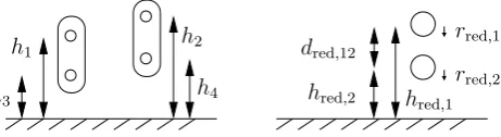
The heights above ground of the equivalent conductors can be estimated by taking the average of the heights of all the conductors of the belonging group (cf. fig. 6):
hred,i= 1 n
n X
k=1
hk, (8)
withn: number of wires in groupi.
h1
h3
rred,1
rred,2
h2
h4
dred,12
hred,1
hred,2
Fig. 6.Geometry of the original (left) and reduced (right) cable
The radii of the equivalent wires can be determined by the conversion of the analytical formula of the self inductance
L0red,ii:
L0red,ii= µ 2πln
2hred,i−rred,i
rred,i
. (9)
The equation for the mutual inductance (concerning the conductorsi,j) can be used to determine the distancedred,ij between two equivalent conductors:
L0red,ij= µ 2πln
d
red,ij−rred,j
s2−rred,j
, (10)
with:
s2=
q
(hred,i+hred,j)2+dred2 ,ij−(hred,j−hred,i)2,
withdred,ijbeing the distance between conductoriand con-ductor j. The distance between the mirror image of con-ductori(because of the metallic ground) and conductorjis nameds2.
6.2 Optimization of the geometry
If we use the results of the geometry parameters as described in chapter 6.1 for further susceptibility calculations of asym-metric signal lines (return conductor: ground), we get quite a good accordance of the sum of the induced currents of the original and the current of the reduced cable bundle. Applying this method to differential cables and particularly to twisted pairs, the accordance is getting very poor. Be-sides, the results of the first estimation usually are not co-herent. Looking at them in detail, we find out that the dis-tance dred,ij, calculated from (10), and the distance which
can be derived from the difference of the hred,i, hred,j are not equal. This comparison can only be done if we use a ge-ometry where the two wires of a pair are located above each other. This is a restriction if uniform lines are analyzed, but is no problem when stepping over to twisted pairs.
The contradiction of the incoherent geometry parameters can be solved by applying an optimization algorithm on the estimates. The estimated values, calculated above, individ-ually match the corresponding inductance matrix perfectly well (where they were derived from). But the geometry of the simplified cable bundle, associated to the matrix, is not unambiguous and the geometry parameters of the first esti-mation do not necessarily match to each other. So, the task is, to find a solution where all parameters harmonize and all conditions (8, 9, 10) are still fulfilled.
The capacitance matrixCred0 does not provide further in-formation if a homogene dielectric is assumed, becauseL0red
andCred0 are directly connected via the propagation velocity:
Cred0 = 1 v2L
0−1
red. (11)
We can state the following conditions, which have to be satisfied by the optimization:
1. The distances of the wires of the reduced cable bundle equal the differences of the first estimates of the heights of the reduced cable bundle, (8): dred,ij=|hred,i−
hred,j|. That means thatdred,ijremains unchanged dur-ing the optimization process. This startdur-ing condition guarantees, that the total diameter of the equivalent ca-ble remains the same, compared to the original caca-ble.
2. Asdred,ijis fixed, thehred,i,hred,jhave to be modified to fulfilldred,ij=|hred,i−hred,j|.
3. When the optimization process in finished, the final re-duced geometry still has to correspond to the the line parameters of the reduced cable bundle (cf. 8, 9, 10). Fig. 6. Geometry of the original (left) and reduced (right) cable.
C0red=
C11+C12+C21+C22 C13+C14+C23+C24
C31+C32+C41+C42 C33+C34+C43+C44
0
,
L0red=
L11+L12+L21+L22
4
L13+L14+L23+L24
4
L31+L32+L41+L42
4
L33+L34+L43+L44
4
0
.
This yields a reduced cable bundle with only two equivalent wires with a reduced capacitance matrix C0redand a reduced inductance matrix L0red.
5 Termination loads
If we focus on differential signals, we consider only differen-tial termination loads, too. Arranging the wires of the differ-ent pairs to various groups, the differdiffer-ential terminations are set in parallel. So, the resulting terminations of the equivalent pairs equal the parallel connections of the belonging original terminations.
6 Geometry of the reduced cable bundle
Following the procedure presented in the previous chapter, we get the system of differential equations (Eq. 7) that char-acterizes the reduced cable bundle. If we want to use field simulation tools on the reduced cable bundle we need to ex-tract the resulting geometry of the reduced cable bundle from the determined p.u.l. (per-unit-length) line parameters. This can be done by the following procedure. It was developed for symmetric signal lines, but can also applied to asymmet-ric ones.
6.1 Determination of estimates
The heights above ground of the equivalent conductors can be estimated by taking the average of the heights of all the conductors of the belonging group (cf. Fig. 6):
hred,i= 1
n
n
X
k=1
hk, (8)
withn: number of wires in groupi.
The radii of the equivalent wires can be determined by the conversion of the analytical formula of the self inductance
L0red,ii:
L0red,ii= µ 2πln
2hred,i−rred,i
rred,i
. (9)
The equation for the mutual inductance (concerning the conductorsi,j) can be used to determine the distancedred,ij between two equivalent conductors:
L0red,ij= µ 2πln
d
red,ij−rred,j
s2−rred,j
, (10)
with:
s2=
q
(hred,i+hred,j)2+dred,ij2 −(hred,j−hred,i)2,
withdred,ij being the distance between conductoriand con-ductor j. The distance between the mirror image of con-ductori(because of the metallic ground) and conductorj is nameds2.
6.2 Optimization of the geometry
If we use the results of the geometry parameters as described in Sect. 6.1 for further susceptibility calculations of asym-metric signal lines (return conductor: ground), we get quite a good accordance of the sum of the induced currents of the original and the current of the reduced cable bundle. Ap-plying this method to differential cables and particularly to twisted pairs, the accordance is getting very poor. Besides, the results of the first estimation usually are not coherent. Looking at them in detail, we find out that the distancedred,ij, calculated from Eq. (10), and the distance which can be de-rived from the difference of thehred,i,hred,j are not equal. This comparison can only be done if we use a geometry where the two wires of a pair are located above each other. This is a restriction if uniform lines are analyzed, but is no problem when stepping over to twisted pairs.
The contradiction of the incoherent geometry parameters can be solved by applying an optimization algorithm on the estimates. The estimated values, calculated above, individ-ually match the corresponding inductance matrix perfectly well (where they were derived from). But the geometry of the simplified cable bundle, associated to the matrix, is not unambiguous and the geometry parameters of the first esti-mation do not necessarily match to each other. So, the task is, to find a solution where all parameters harmonize and all Eqs. (8, 9, 10) are still fulfilled.
The capacitance matrix C0reddoes not provide further in-formation if a homogene dielectric is assumed, because L0red and C0redare directly connected via the propagation velocity:
C0red= 1
v2L
0−1
B. Schetelig et al.: EM field coupling to complex cable bundles 215 We can state the following conditions, which have to be
satisfied by the optimization:
1. The distances of the wires of the reduced cable bun-dle equal the differences of the first estimates of the heights of the reduced cable bundle, Eq. (8): dred,ij= |hred,i−hred,j|. That means that dred,ij remains un-changed during the optimization process. This start-ing condition guarantees, that the total diameter of the equivalent cable remains the same, compared to the original cable.
2. Asdred,ij is fixed, thehred,i,hred,j have to be modified to fulfilldred,ij= |hred,i−hred,j|.
3. When the optimization process in finished, the final re-duced geometry still has to correspond to the the line parameters of the reduced cable bundle (cf. Eqs. 8, 9, 10).
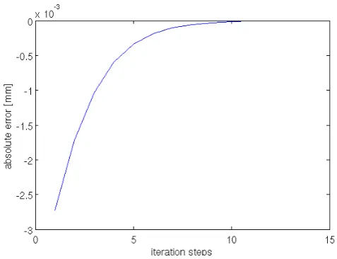
Using these conditions, the optimization procedure is struc-tured as follows:
1. Estimatehred,i,hred,jas the average of the original con-ductors of the corresponding group.
2. Setdred,ijfix as defined in Eq. (1) according to the orig-inal geometry.
3. Recalculate the heighthred,i of the lower wirei, using
dred,ijfrom Eq. (2) andhred,j by applying Eq. (10). 4. Now, the error can be calculated by comparing the
dif-ference of the heights with distancedred,ij Eq. (2). 5. If the error exceeds the predefined tolerance, the height
hred,j of the upper wire j is adjusted by adding (sub-tracting) a portion of the error, depending on the polar-ity of the calculated error
6. A next iterative loop is started by continuing with Eq. (3).
After some steps and according to the defined tolerance, the curve convergences, as to be seen in Fig. 7.
There are different ways of implementing the conditions mentioned above. They result in a different number of nec-essary steps to reach the convergence condition. It is very likely to get different results for the geometry of the reduced cable bundle with little differences in coupling behaviour. The variation presented here, is a very simple one, producing quite good results (see Sect. 8).
By applying this code, a second problem to be mentioned is solved, too. During the reduction of the cable bundle, the radii of the simplified cable tend to grow. This depends on the reduction of theL0ii(cf. Eq. 12) when moving from Eq. (6) to Eq. (7). As a consequence it is not possible to apply the cable reduction technique if the original cables have very lit-tle distance, since the reduced cable would overlap. When
Using these conditions, the optimization procedure is struc-tured as follows:
1. Estimatehred,i,hred,jas the average of the original con-ductors of the corresponding group.
2. Setdred,ij fix as defined in condition 1 according to the original geometry.
3. Recalculate the heighthred,i of the lower wirei, using
dred,ijfrom step 2 andhred,jby applying (10).
4. Now, the error can be calculated by comparing the dif-ference of the heights with distancedred,ij (step 2).
5. If the error exceeds the predefined tolerance, the height
hred,j of the upper wire j is adjusted by adding (sub-tracting) a portion of the error, depending on the polar-ity of the calculated error
6. A next iterative loop is started by continuing with step 3.
After some steps and according to the defined tolerance, the curve convergences, as to be seen in fig. 7.
Fig. 7.Error reduction due to recursive iterations
There are different ways of implementing the conditions mentioned above. They result in a different number of nec-essary steps to reach the convergence condition. It is very likely to get different results for the geometry of the reduced cable bundle with little differences in coupling behaviour. The variation presented here, is a very simple one, producing quite good results (see chapter 8).
By applying this code, a second problem to be mentioned is solved, too. During the reduction of the cable bundle, the radii of the simplified cable tend to grow. This depends on the reduction of theL0ii (cf. (12)) when moving from (6) to (7). As a consequence it is not possible to apply the cable reduc-tion technique if the original cables have very little distance, since the reduced cable would overlap. When the geometry
is varied recursively in the context of the optimization code, the heights are reduced, compared to the first estimate of the reduced geometry, and as (12) shows, the result is a reduction of the radii, too:
rred,i=
2·hred,i
exp L0
red,ii·2π
µ
. (12)
We know from experience that it is even possible to cut away the overlapping radii (without touching the distance) to about 70% causing quite little error.
7 Twisted-pair cables
The application of this procedure on twisted-pair cables seems to be very difficult at the beginning: The procedure described above depends on the line parameters of the origi-nal as well as the reduced cable. The determination of these parameters initially requires, by definition, a homogene ge-ometry with a constant distance to the ground. That is not the case for twisted cables. There are several studies that have a close look at the problem how to apply transmission line the-ory to nonuniform cables. (Nitsch and Gronwald, 1999) uses a generalized telegrapher’s equation. (Omid, 1997) adopts a method of an equivalent cascaded network chain. In the con-text of reduction of twisted-pair cables, a much more simple methodology can be applied and leads to satisfying results.
The approach is based on a chained transmission line anal-ysis too. What we are looking for is the replacement of a large bundle of twisted pairs by a reduced bundle with only one twisted pair (fig. 8). This is an enormous simplification of the nonuniform structure.
A
A
B
B
P
air
1
P
air
2
Fig. 8. Principle of reducing twisted-pair cables: Original cable bundle (left) and reduced cable (right)
To demonstrate this simplification approach, we want to analyze one twist of the original cable. The 360◦ twist is divided exemplarily into four parts (angle of difference ∆α= 90◦), as illustrated in fig. 9. These parts can now be regarded separately. We reduce the twisted pairs in each part of the twist in the way as shown on the left side of fig. 8. The arrangement of the wires is done in the same way as it is done with uniform cables. When we now have a look at the geometry of the reduced system, we see that the reduction of twisted pairs yields a twisted pair again. This is because Fig. 7. Error reduction due to recursive iterations.
the geometry is varied recursively in the context of the opti-mization code, the heights are reduced, compared to the first estimate of the reduced geometry, and as Eq. (12) shows, the result is a reduction of the radii, too:
rred,i=
2·hred,i exp L
0 red,ii·2π
µ
!. (12)
We know from experience that it is even possible to cut away the overlapping radii (without touching the distance) to about 70% causing quite little error.
7 Twisted-pair cables
The application of this procedure on twisted-pair cables seems to be very difficult at the beginning: The procedure described above depends on the line parameters of the origi-nal as well as the reduced cable. The determination of these parameters initially requires, by definition, a homogene ge-ometry with a constant distance to the ground. That is not the case for twisted cables. There are several studies that have a close look at the problem how to apply transmission line the-ory to nonuniform cables. (Nitsch and Gronwald, 1999) uses a generalized telegrapher’s equation. (Omid, 1997) adopts a method of an equivalent cascaded network chain. In the con-text of reduction of twisted-pair cables, a much more simple methodology can be applied and leads to satisfying results.
The approach is based on a chained transmission line anal-ysis too. What we are looking for is the replacement of a large bundle of twisted pairs by a reduced bundle with only one twisted pair (Fig. 8). This is an enormous simplification of the nonuniform structure.
216 B. Schetelig et al.: EM field coupling to complex cable bundles Using these conditions, the optimization procedure is
struc-tured as follows:
1. Estimatehred,i,hred,jas the average of the original con-ductors of the corresponding group.
2. Setdred,ij fix as defined in condition 1 according to the original geometry.
3. Recalculate the heighthred,i of the lower wirei, using
dred,ijfrom step 2 andhred,jby applying (10).
4. Now, the error can be calculated by comparing the dif-ference of the heights with distancedred,ij (step 2).
5. If the error exceeds the predefined tolerance, the height
hred,j of the upper wirej is adjusted by adding (sub-tracting) a portion of the error, depending on the polar-ity of the calculated error
6. A next iterative loop is started by continuing with step 3.
After some steps and according to the defined tolerance, the curve convergences, as to be seen in fig. 7.
Fig. 7.Error reduction due to recursive iterations
There are different ways of implementing the conditions mentioned above. They result in a different number of nec-essary steps to reach the convergence condition. It is very likely to get different results for the geometry of the reduced cable bundle with little differences in coupling behaviour. The variation presented here, is a very simple one, producing quite good results (see chapter 8).
By applying this code, a second problem to be mentioned is solved, too. During the reduction of the cable bundle, the radii of the simplified cable tend to grow. This depends on the reduction of theL0ii(cf. (12)) when moving from (6) to (7). As a consequence it is not possible to apply the cable reduc-tion technique if the original cables have very little distance, since the reduced cable would overlap. When the geometry
is varied recursively in the context of the optimization code, the heights are reduced, compared to the first estimate of the reduced geometry, and as (12) shows, the result is a reduction of the radii, too:
rred,i=
2·hred,i
exp L0
red,ii·2π
µ
. (12)
We know from experience that it is even possible to cut away the overlapping radii (without touching the distance) to about 70% causing quite little error.
7 Twisted-pair cables
The application of this procedure on twisted-pair cables seems to be very difficult at the beginning: The procedure described above depends on the line parameters of the origi-nal as well as the reduced cable. The determination of these parameters initially requires, by definition, a homogene ge-ometry with a constant distance to the ground. That is not the case for twisted cables. There are several studies that have a close look at the problem how to apply transmission line the-ory to nonuniform cables. (Nitsch and Gronwald, 1999) uses a generalized telegrapher’s equation. (Omid, 1997) adopts a method of an equivalent cascaded network chain. In the con-text of reduction of twisted-pair cables, a much more simple methodology can be applied and leads to satisfying results.
The approach is based on a chained transmission line anal-ysis too. What we are looking for is the replacement of a large bundle of twisted pairs by a reduced bundle with only one twisted pair (fig. 8). This is an enormous simplification of the nonuniform structure.
A
A
B
B
P
air
1
P
air
2
Fig. 8. Principle of reducing twisted-pair cables: Original cable bundle (left) and reduced cable (right)
To demonstrate this simplification approach, we want to analyze one twist of the original cable. The 360◦ twist is divided exemplarily into four parts (angle of difference ∆α= 90◦), as illustrated in fig. 9. These parts can now be regarded separately. We reduce the twisted pairs in each part of the twist in the way as shown on the left side of fig. 8. The arrangement of the wires is done in the same way as it is done with uniform cables. When we now have a look at the geometry of the reduced system, we see that the reduction of twisted pairs yields a twisted pair again. This is because Fig. 8. Principle of reducing twisted-pair cables: Original cable bundle (left) and reduced cable (right).
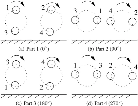
To demonstrate this simplification approach, we want to analyze one twist of the original cable. The 360◦ twist is divided exemplarily into four parts (angle of difference
1α=90◦), as illustrated in Fig. 9. These parts can now be regarded separately. We reduce the twisted pairs in each part of the twist in the way as shown on the left side of Fig. 8. The arrangement of the wires is done in the same way as it is done with uniform cables. When we now have a look at the geometry of the reduced system, we see that the reduction of twisted pairs yields a twisted pair again. This is because the wires we group together always have the same relation to each other in every position of the twist. This can been seen exemplarily in Fig. 9 for four steps. Of course, because of the change of height of each wire, the resulting radii of the reduced cable are not exactly the same. As the difference can be neglected in practical configurations, these radii can be averaged. Hence, it is possible to simplify cable bundles with several twisted pairs to reduced ones with only one pair. Additionally, it is possible to perform the total reduction pro-cess and the calculation of the reduced geometry only on the geometry of part 1 of Fig. 9. The results then can be used to model the reduced twisted pair in the CAD environment of the field simulation tool. In this way, it possible to treat twisted-pair cables during the reduction process in the same way as uniform cables, if the pitch length (incl. orientation) as well as the wire distances of the different original pairs are the same. If one of these criteria is violated, the resulting equivalent cable pair is no longer an ideal helix structure and averaging had to be applied.
8 Validation
To verify the presented method, a MATLAB script was im-plemented to cover the total reduction process starting with the original geometry and ending with the reduced geometry. The total procedure of reduction is structured as follows:
1. Analytic calculation of the line parameters according to the original geometry.
2. Generation of the line parameters of the reduced cable bundle from the original cable bundle.
6 B. Schetelig et al.: EM Field Coupling to Complex Cable Bundles
the wires we group together always have the same relation to each other in every position of the twist. This can been seen exemplarily in fig. 9 for four steps. Of course, because of the change of height of each wire, the resulting radii of the reduced cable are not exactly the same. As the difference can be neglected in practical configurations, these radii can be averaged. Hence, it is possible to simplify cable bundles with several twisted pairs to reduced ones with only one pair. Additionally, it is possible to perform the total reduction pro-cess and the calculation of the reduced geometry only on the geometry of part 1 of fig. 9. The results then can be used to model the reduced twisted pair in the CAD environment of the field simulation tool. In this way, it possible to treat twisted-pair cables during the reduction process in the same way as uniform cables, if the pitch length (incl. orientation) as well as the wire distances of the different original pairs are the same. If one of these criteria is violated, the resulting equivalent cable pair is no longer an ideal helix structure and averaging had to be applied.
1
2
3
4
(a) Part 1 (0◦)
1
3
4
2
(b) Part 2 (90◦)
3
4
1
2
(c) Part 3 (180◦)
3
1
2
4
(d) Part 4 (270◦)
Fig. 9.Stepwise analysis of a360◦twist of a twisted-pair cable
8 Validation
To verify the presented method, a MATLAB script was im-plemented to cover the total reduction process starting with the original geometry and ending with the reduced geometry. The total procedure of reduction is structured as follows:
1. Analytic calculation of the line parameters according to the original geometry.
2. Generation of the line parameters of the reduced cable bundle from the original cable bundle.
3. First estimation of the geometry of the reduced cable by applying the same equations as in step 1.
4. Application of the iterative optimization run.
5. Modelling the reduced geometry in a 3D field simula-tion program (FEKO) and comparing the induced cur-rents to the curcur-rents from the simulation run of the orig-inal cable.
The basic geometrical parameters of the original cable used for the following validations are:
height of the lower wire 5 mm
wire radius 0.1 mm
distance between twisted wires 0.5 mm distance between two pairs 0.5 mm length of twist (for twisted pairs) 20 mm
The excitation of the transmission lines is a vertically po-larized plane EM wave with a poynting vector perpendicular to the cable bundle.
First, we want to compare the results for differential pairs of uniform wires. In fig. 10, the currents in the original and reduced cable bundles are plotted. Note the good accordance between the curves. The amplitudes as well as the resonance peaks match very well.
Fig. 10.Comparison of the induced current on a uniform, differen-tial cable
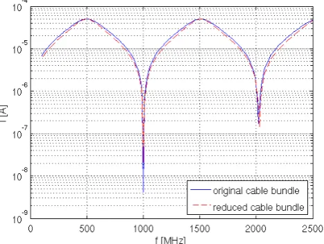
Fig. 11 shows the comparison of the currents in the orig-inal and the reduced twisted harness. As we can see, the curves match quite well. There is only a little difference in the resonance peaks. This can be explained by the fact, that by reducing the cable, the propagation velocity is shifted a tiny amount.
v2=L0−1·C0−1 (13)
This is because the product of the p.u.l.-parametersL0origand
Corig0 of the original cable does not equal the product L0red
andCred0 of the reduced cable. One way to improve the ac-cordance is to add a dielectric coating to the wires of the Fig. 9. Stepwise analysis of a 360◦twist of a twisted-pair cable.
3. First estimation of the geometry of the reduced cable by applying the same equations as in Eq. (1).
4. Application of the iterative optimization run.
5. Modelling the reduced geometry in a 3D field simula-tion program (FEKO) and comparing the induced cur-rents to the curcur-rents from the simulation run of the orig-inal cable.
The basic geometrical parameters of the original cable used for the following validations are:
height of the lower wire 5 mm
wire radius 0.1 mm
distance between twisted wires 0.5 mm distance between two pairs 0.5 mm length of twist (for twisted pairs) 20 mm
The excitation of the transmission lines is a vertically po-larized plane EM wave with a poynting vector perpendicular to the cable bundle.
First, we want to compare the results for differential pairs of uniform wires. In Fig. 10, the currents in the original and reduced cable bundles are plotted. Note the good accordance between the curves. The amplitudes as well as the resonance peaks match very well.
Figure 11 shows the comparison of the currents in the orig-inal and the reduced twisted harness. As we can see, the curves match quite well. There is only a little difference in the resonance peaks. This can be explained by the fact, that by reducing the cable, the propagation velocity is shifted a tiny amount.
B. Schetelig et al.: EM field coupling to complex cable bundles 217
the wires we group together always have the same relation to each other in every position of the twist. This can been seen exemplarily in fig. 9 for four steps. Of course, because of the change of height of each wire, the resulting radii of the reduced cable are not exactly the same. As the difference can be neglected in practical configurations, these radii can be averaged. Hence, it is possible to simplify cable bundles with several twisted pairs to reduced ones with only one pair. Additionally, it is possible to perform the total reduction pro-cess and the calculation of the reduced geometry only on the geometry of part 1 of fig. 9. The results then can be used to model the reduced twisted pair in the CAD environment of the field simulation tool. In this way, it possible to treat twisted-pair cables during the reduction process in the same way as uniform cables, if the pitch length (incl. orientation) as well as the wire distances of the different original pairs are the same. If one of these criteria is violated, the resulting equivalent cable pair is no longer an ideal helix structure and averaging had to be applied.
1
2
3
4
(a) Part 1 (0◦)
1
3
4
2
(b) Part 2 (90◦)
3
4
1
2
(c) Part 3 (180◦)
3
1
2
4
(d) Part 4 (270◦)
Fig. 9.Stepwise analysis of a360◦twist of a twisted-pair cable
8 Validation
To verify the presented method, a MATLAB script was im-plemented to cover the total reduction process starting with the original geometry and ending with the reduced geometry. The total procedure of reduction is structured as follows:
1. Analytic calculation of the line parameters according to the original geometry.
2. Generation of the line parameters of the reduced cable bundle from the original cable bundle.
3. First estimation of the geometry of the reduced cable by applying the same equations as in step 1.
4. Application of the iterative optimization run.
5. Modelling the reduced geometry in a 3D field simula-tion program (FEKO) and comparing the induced cur-rents to the curcur-rents from the simulation run of the orig-inal cable.
The basic geometrical parameters of the original cable used for the following validations are:
height of the lower wire 5 mm
wire radius 0.1 mm
distance between twisted wires 0.5 mm
distance between two pairs 0.5 mm
length of twist (for twisted pairs) 20 mm
The excitation of the transmission lines is a vertically po-larized plane EM wave with a poynting vector perpendicular to the cable bundle.
First, we want to compare the results for differential pairs of uniform wires. In fig. 10, the currents in the original and reduced cable bundles are plotted. Note the good accordance between the curves. The amplitudes as well as the resonance peaks match very well.
Fig. 10.Comparison of the induced current on a uniform, differen-tial cable
Fig. 11 shows the comparison of the currents in the orig-inal and the reduced twisted harness. As we can see, the curves match quite well. There is only a little difference in the resonance peaks. This can be explained by the fact, that by reducing the cable, the propagation velocity is shifted a tiny amount.
v2=L0−1·C0−1 (13) This is because the product of the p.u.l.-parametersL0origand Corig0 of the original cable does not equal the productL0red andCred0 of the reduced cable. One way to improve the ac-cordance is to add a dielectric coating to the wires of the
Fig. 10. Comparison of the induced current on a uniform, differen-tial cable.
This is because the product of the p.u.l.-parameters L0orig and C0
orig of the original cable does not equal the product L0
redand C0redof the reduced cable. One way to improve the accordance is to add a dielectric coating to the wires of the reduced cable bundle (Andrieu, 2006). This would affect the capacitance and in that way, the propagation velocity of the reduced cable could be adapted.
Finally, we want to review the improved possibility to ap-ply the reduction method to cables with wires that are situ-ated very close to each other. The advantage can be summa-rized as a reduced growth of the radii in the context of the simplification. The radii of the simplified cable in this ex-ample arerred,est = 0.32 mm if the optimization algorithm is not applied. If the optimized geometry data is used, the radii are reduced to an average ofrred,opt = 0.21 mm. This means a reduction to 66% of the original size and the arising space between the wire can be used for a narrower adjust-ment of the original cable bundle. The agreeadjust-ment between the original and the reduced cable bundles still remains good as shown in Figs. 10 and 11.
9 Conclusions
In this paper an approach was derived to extend the Equiv-alent Cable Bundle Method to differential cables. We pre-sented an optimization algorithm that enabled the application on twisted-pair cables and the analysis of cable bundles with very little distance between the wires. As shown in the vali-dation chapter, this methodology yields to a good accordance of the simplified cable bundle with the original one. Hence, the methodology allows to perform a simplified modelling of EM fields to differential transmission lines.
B. Schetelig et al.: EM Field Coupling to Complex Cable Bundles 7
reduced cable bundle (Andrieu, 2006). This would affect the capacitance and in that way, the propagation velocity of the reduced cable could be adapted.
Fig. 11.Comparison of the induced current on a twisted-pair cable
Finally, we want to review the improved possibility to ap-ply the reduction method to cables with wires that are situ-ated very close to each other. The advantage can be summa-rized as a reduced growth of the radii in the context of the simplification. The radii of the simplified cable in this ex-ample arerred,est = 0.32 mmif the optimization algorithm
is not applied. If the optimized geometry data is used, the radii are reduced to an average ofrred,opt = 0.21 mm. This
means a reduction to 66% of the original size and the arising space between the wire can be used for a narrower adjust-ment of the original cable bundle. The agreeadjust-ment between the original and the reduced cable bundles still remains good as shown in fig. 10 and fig. 11.
9 Conclusions
In this paper an approach was derived to extend the Equiv-alent Cable Bundle Method to differential cables. We pre-sented an optimization algorithm that enabled the application on twisted-pair cables and the analysis of cable bundles with very little distance between the wires. As shown in the vali-dation chapter, this methodology yields to a good accordance of the simplified cable bundle with the original one. Hence, the methodology allows to perform a simplified modelling of EM fields to differential transmission lines.
References
Andrieu, G.: Elaboration et application d’une m´ethode de fais-ceau ´equivalent pour l’´etude des couplages ´electromagnetiques
sur r´eseaux de cˆablages automobiles, Ph.D. thesis, Lille Univer-sity, 2006.
Andrieu, G., Kon´e, L., Bocquet, F., D´emoulin, B., and Par-mantier, J.-P.: Multiconductor Reduction Technique for Mod-eling Common-Mode Currents on Cable Bundles at High Fre-quency for Automotive Applications, IEEE Transactions on elec-tromagnetic compatibility, 50, 175–184, 2008.
Nitsch, J. and Gronwald, F.: Analytical Solutions in Nonuniform Multiconductor Transmission Line Theory, IEEE Transactions on electromagnetic compatibility, 41, 469–479, 1999.
Omid, M.: Field Coupling to Nonuniform and Uniform Transmis-sion Lines, IEEE Transactions on electromagnetic compatibility, 39, 201–211, 1997.
Paul, C. R.: Analysis of Multiconductor Transmission Lines, Wiley, 1994.
Tesche, F. M.: Principles and applications of EM field coupling to transmission lines, EMC Zurich Symposium, 9, 21–31, 1995. Tesche, F. M., Ianoz, M. V., and Karlsson, T.: EMC Analysis
Meth-ods and Computational MethMeth-ods, Wiley, 1997.
Fig. 11. Comparison of the induced current on a twisted-pair cable.
References
Andrieu, G.: Elaboration et application d’une m´ethode de fais-ceau ´equivalent pour l’´etude des couplages ´electromagnetiques sur r´eseaux de cˆablages automobiles, Ph.D. thesis, Lille Univer-sity, 2006.
Andrieu, G., Kon´e, L., Bocquet, F., D´emoulin, B., and Par-mantier, J.-P.: Multiconductor Reduction Technique for Mod-eling Common-Mode Currents on Cable Bundles at High Fre-quency for Automotive Applications, IEEE Transactions on elec-tromagnetic compatibility, 50, 175–184, 2008.
Nitsch, J. and Gronwald, F.: Analytical Solutions in Nonuniform Multiconductor Transmission Line Theory, IEEE Transactions on electromagnetic compatibility, 41, 469–479, 1999.
Omid, M.: Field Coupling to Nonuniform and Uniform Transmis-sion Lines, IEEE Transactions on electromagnetic compatibility, 39, 201–211, 1997.
Paul, C. R.: Analysis of Multiconductor Transmission Lines, Wiley, 1994.
Tesche, F. M.: Principles and applications of EM field coupling to transmission lines, EMC Zurich Symposium, 9, 21–31, 1995. Tesche, F. M., Ianoz, M. V., and Karlsson, T.: EMC Analysis
Meth-ods and Computational MethMeth-ods, Wiley, 1997.