The Thirty-Third AAAI Conference on Artificial Intelligence (AAAI-19)
B´ezier Simplex Fitting: Describing Pareto Fronts of
Simplicial Problems with Small Samples in Multi-Objective Optimization
Ken Kobayashi,
1,2Naoki Hamada,
1,2Akiyoshi Sannai,
2,3Akinori Tanaka,
2,3Kenichi Bannai,
3,2Masashi Sugiyama
2,41Artificial Intelligence Laboratory, Fujitsu Laboratories Ltd., Japan 2The Center for Advanced Intelligence Project, RIKEN, Japan
3Department of Mathematics, Faculty of Science and Technology, Keio University, Japan
4Department of Complexity Science and Engineering, Graduate School of Frontier Sciences, The University of Tokyo, Japan
Abstract
Multi-objective optimization problems require simultane-ously optimizing two or more objective functions. Many stud-ies have reported that the solution set of an M-objective optimization problem often forms an(M −1)-dimensional topological simplex (a curved line for M = 2, a curved triangle for M = 3, a curved tetrahedron for M = 4, etc.). Since the dimensionality of the solution set increases as the number of objectives grows, an exponentially large sample size is needed to cover the solution set. To reduce the required sample size, this paper proposes a B´ezier sim-plex model and its fitting algorithm. These techniques can exploit the simplex structure of the solution set and de-compose a high-dimensional surface fitting task into a se-quence of low-dimensional ones. An approximation theorem of B´ezier simplices is proven. Numerical experiments with synthetic and real-world optimization problems demonstrate that the proposed method achieves an accurate approxima-tion of high-dimensional soluapproxima-tion sets with small samples. In practice, such an approximation will be conducted in the post-optimization process and enable a better trade-off analysis.
Introduction
A multi-objective optimization problem is a problem that minimizes multiple objective functionsf1, . . . , fM : X → Rover a common domainX ⊆RL:
minimizef(x) := (f1(x), . . . , fM(x)) subject tox∈X.
Different functions usually have different minimizers, and one needs to consider a trade-off that two solutionsx,y ∈
X may satisfyfi(x)< fi(y)andfj(x)> fj(y). Accord-ing toPareto ordering, i.e.,
f(x)≺f(y)⇐⇒def fm(x)≤fm(y)for allm= 1, . . . , M andfm(x)< fm(y)for somem= 1, . . . , M, the goal of multi-objective optimization is to obtain the
Pareto set
X∗(f) :={x∈X |f(y)6≺f(x)for ally∈X} and thePareto front
fX∗(f) :=
f(x)∈RM x∈X∗(f)
Copyright c2019, Association for the Advancement of Artificial Intelligence (www.aaai.org). All rights reserved.
which describe the best-compromising solutions and their values of the conflicting objective functions, respectively.
In industrial applications, obtaining the whole Pareto set/front rather than a single solution enables us to com-pare promising alternatives and to explore new innovative designs, whose concept is variously refered to as innoviza-tion (Deb and Srinivasan 2006), multi-objective design ex-ploration (Obayashi, Jeong, and Chiba 2005) and design informatics (Chiba, Makino, and Takatoya 2009). Quite a few real-world problems involve simulations and/or exper-iments to evaluate solutions (Chand and Wagner 2015) and lack the mathematical expression of their objective functions and derivatives. Multi-objective evolutionary algorithms are a tool to solve such problems where the Pareto set/front is approximated by a population, i.e., a finite set of sample points (Coello, Lamont, and Van Veldhuisen 2007).
While the available sample size is limited due to expen-sive simulations and experiments, it is well-known that the dimensionality of the Pareto set/front increases as the num-ber of objectives grows. Describing high-dimensional Pareto sets/fronts with small samples is one of the key challenges in many-objective optimization today (Li et al. 2015).
A considerable number of real-world applications share an interesting structure: their Pareto sets and/or Pareto fronts are often homeomorphic to an(M −1)-dimensional sim-plex. See for example (Rodr´ıguez-Ch´ıa and Puerto 2002; Vrugt et al. 2003; Shoval et al. 2012; Mastroddi and Gemma 2013). This observation has been theoretically backed up in some cases (Kuhn 1967; Smale 1973; Shoval et al. 2012). A recent study (Lovison and Pecci 2014) pointed out that for allm ≤ M, each(m−1)-dimensional face of such a simplex is the Pareto set of a subproblem optimizingm ob-jective functions of the original problem.
(a) Simplex∆J (b) Pareto setX∗(fJ) (c) Pareto frontfX∗(fJ)
Figure 1: Skeletons for non-emptyJ ⊆ {1,2,3}and simplicialf = (f1, f2, f3).
Our contibution can be summarized as follows:
1. We define a new class of multi-objective optimization problems called the simplicial problem in which the Pareto set/front have the simplex structure discussed above. We propose a B´ezier simplex model, which is a generalization of a B´ezier curve (Farin 2002).
2. We prove that B´ezier simplices can approximate the Pareto set/front (as well as the objective map between them) of any simplicial problem with arbitrary accuracy.
3. We propose a B´ezier simplex fitting algorithm. Exploiting the simplex structure of the Pareto set/front of a simplicial problem, this algorithm decomposes a B´ezier simplex into low-dimensional simplices and fits each of them, induc-tively. This approach allows us to reduce the number of parameters to be estimated at a time.
4. We evaluate the approximation accuracy of the proposed method with synthetic and real-world optimization prob-lems; compared to a conventional response surface model for Pareto fronts, our method exhibits a better boundary approximation while keeping the almost same quality of interior approximation. As a result, a five-objective Pareto front is described with only tens of sample points.
Preliminaries
Let us introduce notations for defining simplicial problems and review an existing method of B´ezier curve fitting.
Simplicial Problem
A multi-objective optimization problem is denoted by its objective map f = (f1, . . . , fM) : X → RM. Let I := {1, . . . , M}be the index set of objective functions and
∆M−1:=
(
(t1, . . . , tM)∈RM
0≤tm,
X
m∈M
tm= 1
)
be thestandard simplexinRM. For each non-empty subset
J ⊆I, we call
∆J :=(t1, . . . , tM)∈∆M−1
tm= 0 (m6∈J)
theJ-faceof∆M−1(see Figure 1a) and
fJ := (fi)i∈J:X→R|J|
theJ-subproblemoff. For each0≤m≤M −1, we call
∆(m):= [
J⊆I,|J|=m
∆J
them-skeletonof∆M−1.
The problem class we are interested in is as follows:
Definition 1 (Simplicial problem) A problem f : X →
RM is simplicialif there exists a map φ : ∆M−1 → X
such that for each non-empty subsetJ ⊆ I, its restriction
φ|∆J : ∆J→X gives homeomorphisms
φ|∆J : ∆J→X∗(fJ), f◦φ|∆J : ∆J→fX∗(fJ).
We call such φ and f ◦ φ a triangulation of the Pareto setX∗(f)and the Pareto frontfX∗(f), respectively. For each non-empty subsetJ ⊆ I, we callX∗(fJ)the J-face
ofX∗(f)and fX∗(fJ)the J-faceoffX∗(f). For each
0≤m≤M−1, we call
X∗(m):= [
J⊆I,|J|=m
X∗(fJ),
fX∗(m):= [
J⊆I,|J|=m
fX∗(fJ)
them-skeletonofX∗(f)andfX∗(f), respectively.
By definition, any subproblem of a simplicial problem is again simplicial. The homeomorphism φ|∆J ensures that the Pareto sets forms a curved simplex as shown in Fig-ure 1b. The homeomorphismf◦φ|∆Jasserts thatf|X∗(f):
X∗(f) →
The above structure appears in a broad range of appli-cations. In operations research, the Pareto set of the facil-ity location problem under theL2-norm is shown to be the convex hull of single-objective optima (Kuhn 1967). When the optima are in general position, the Pareto set becomes a simplex. Similar observations are also reported under other norms (Rodr´ıguez-Ch´ıa and Puerto 2002). In economics, the Pareto set of the pure exchange economy withM players is known to be homeomorphic to an(M−1)-dimensional sim-plex (Smale 1973). In hydrology, the two-objective Pareto set of a hydrologic cycle model calibration is observed to be a curve. Its end points are single-objective optima, and the end points correspond to end points of the Pareto front curve (Vrugt et al. 2003). In addition, a recent study pointed out that the Pareto set of anM-objective convex optimiza-tion problem is diffeomorphic to an(M −1)-dimensional simplex and that its(m−1)-dimensional faces are the Pareto sets ofm-objective subproblems for allm ≤ M (Lovison and Pecci 2014).
B´ezier Curve Fitting
Since the Pareto front of any two-objective simplicial prob-lem is a curve with two end points inR3, the B´ezier curve would be a suitable model for describing it.
In RM, the B´ezier curve of degree D is a parametric curve, i.e., a mapb : [0,1] → RM determined byD+ 1
control pointsp0, . . . ,pD∈RM (Farin 2002):
b(t) :=
D
X
d=0
D
d
td(1−t)(D−d)pd (0≤t≤1), (1)
where Ddrepresents the binomial coefficient. The parame-tert moves fromt = 0tot = 1, giving a curveb(t)with two end pointsb(0) =p0andb(1) =pD.
Given sample pointsx1, . . . ,xN ∈ RM, a B´ezier curve can be fitted by solving the following problem (Borges and Pastva 2002):
minimize tn,pd
N
X
n=1
kb(tn)−xnk 2
subject to 0≤tn≤1 (n= 1, . . . , N)
(2)
wheretn (n= 1, . . . , N)andpd(d= 0, . . . , D)are vari-ables to be optimized. Notice thattn (n = 1, . . . , N) are introduced to calculate residuals for each sample point. The error function (2) to be minimized represents the sum of squared residuals for sample points.
If one fix all control pointspd(d= 0, . . . , D), the B´ezier curveb(t)is determined. The error function (2) can be now separately optimized by minimizingkb(tn)−xnk
2 with re-spect to eachtn. The solutiontnis the foot of a perpendicu-lar line from a sample pointxnto the B´ezier curveb([0,1]), which satisfies
∂ ∂t
t=t
n
b(t), b(tn)−xn
= 0. (3)
Since (3) is a nonlinear equation, Newton’s method is used to find the solutiontn.
Algorithm 1B´ezier curve fitting (Borges and Pastva 2002)
1: (Initialize) Seti←1and initial control pointsp(di)(d= 0, . . . , D).
2: whilenot convergeddo
3: (Update parameters) Fix control points p(di) (d = 0, . . . , D)and solve (3) for eachn= 1, . . . , N using Newton’s method. Then set the solutions ast(ni+1).
4: (Update control points) Solve (2) with respect to the control points and set the solutions asp(di+1) (d = 0, . . . , D).
5: i←i+ 1.
6: end while
7: return p(di)(d= 0, . . . , D)
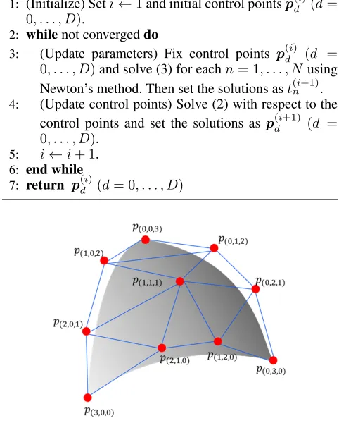
Figure 2: A B´ezier simplex forM = 3,D= 3.
If one fix all parameterstn (n = 1, . . . , N), the B´ezier curve b(tn)becomes a linear function with respect to the control pointsp0, . . . ,pD. The error function (2) can be now optimized by solving linear equations with respect to allpd. Algorithm 1 shows Borges and Pastva’s method, which alternately adjusts parameters and control points. This algo-rithm is also used to adjust some of the control points with remaining points fixed (Shao and Zhou 1996).
B´ezier Simplex Fitting
To describe the Pareto front of an arbitrary-objective sim-plicial problem, however, B´ezier curve fitting is not enough, and we need to generalize it to the B´ezier simplex. We pro-pose a method of fitting a B´ezier simplex to the Pareto front of a simplicial problem.
B´ezier Simplex
LetNbe the set of nonnegative integers and
NMD :=
(
(d1, . . . , dM)∈NM
M
X
m=1
dm=D
)
.
Fort := (t1, . . . , tM) ∈ RM andd := (d1, . . . , dM) ∈ NM, we denote bytda monomialtd11t
d2 2 · · ·t
dM
∆M−1→RM determined by control pointspd∈RM (d∈ NMD):
b(t) := X
d∈NMD
D
d
tdpd, (4)
where Dd
represents a polynomial coefficient
D
d
:= D!
d1!d2!· · ·dM!
.
Approximation Theorem
Is the B´ezier simplex a suitable model for describing the Pareto front of a simplicial problem? Let us check that for any simplicial problem, B´ezier simplices can approximate the Pareto front (as well as the Pareto set and the objective map between them) with arbitrary accuracy.
We begin with a more general proposition that any contin-uous map on a simplex can be uniformly approximated by some B´ezier simplex as a map:
Theorem 1 Letφ : ∆M−1 →
RK be a continuous map.
There exists an infinite sequence of B´ezier simplicesb(i) :
∆M−1→
RKsuch that
lim
i→∞t∈sup∆M−1
|φ(t)−b(i)(t)|= 0.
The proof of Theorem 1 is shown in Appendix A.1
Recall (Definition 1) that a simplicial problemf :X → RM admits a triangulation of the Pareto set
φ: ∆M−1→X∗(f)⊂RL, which induces a triangulation of the Pareto front
f◦φ: ∆M−1→fX∗(f)⊂RM.
Addtionally, the trianglation φ : ∆M−1 → X∗(f)
also induces a triangulation of a restricted objective map f : X∗(f) → fX∗(f). That is, its graph G∗(f) =
(x,f(x))∈RL×
RM x∈X∗(f) is triangulated by
the induced map
(φ,f◦φ) : ∆M−1→G∗(f)⊂RL+M
becausef :X∗(f)→fX∗(f)is continuous by definition and any continuous map induces a homeomorphism from the domain to the graph. These three triangulations fulfill the qualifications of the mapφin Theorem 1. We thus get the desired result for approximation as a set.
Corollary 2 LetX∗ be the Pareto set, the Pareto front or the graph of the objective map restricted to the Pareto set of a simplicial problem. There exists an infinite sequence of B´ezier simplicesb(i): ∆M−1→
RKsuch that
lim
i→∞dH(X
∗, B(i)) = 0
wheredHis the Hausdorff distance andB(i)are images of
B´ezier simplices:B(i):=b(i)(∆M−1). 1
Appendix is available from https://github.com/rafcc/ stratification-learning.
Algorithm 2B´ezier simplex fitting (all-at-once)
1: (Initialize) Seti←1and initial control pointsp(di)(d∈ NMD).
2: whilenot convergeddo
3: (Update parameters) Fix control points p(di) (d ∈ NMD)and solve (6) for eachn= 1, . . . , Nusing New-ton’s method. Then set the solutions ast(ni+1).
4: (Update control points) Solve (5) with respect to the control points and set the solutionsp(di+1)(d∈NMD).
5: i←i+ 1.
6: end while
7: return p(di)(d∈NMD)
All-at-Once Fitting
Let us consider algorithms to realize such a sequence of B´ezier simplices. First, we develop a straightforward gen-eralization of the B´ezier curve fitting method. We call this method theall-at-once fitting.
Given sample pointsx1, . . . ,xN ∈RM, a B´ezier simplex can be fitted by solving the following problem, which is a multi-dimensional analogue of the problem (2):
minimize
tn,pd N
X
n=1
kb(tn)−xnk 2
subject totn ∈∆M−1 (n= 1, . . . , N)
(5)
wheretn = (tn1, . . . , tnM) (n = 1, . . . , N)andpd (d ∈ NMD)are variables to be optimized.
As is the case of B´ezier curve fitting, if one fix all control pointspd(d∈NMD), the B´ezier simplexb(t)is determined. The error function (5) can be now separately optimized by minimizingkb(tn)−xnk2with respect to eachtn. The so-lutiontn is the foot of a perpendicular line from a sample pointxnto the B´ezier simplexb(∆M−1), which satisfies
∂ ∂tm
t=t
n
b(t), b(tn)−xn
= 0 (m= 1, . . . , M).
(6) Since (6) is a system of nonlinear equations, Newton’s method is used to find the solutiontn.
If one fix all parameterstn (n = 1, . . . , N), the B´ezier simplexb(tn)is a linear function with respect to the con-trol points pd (d ∈ NMD). The error function (5) can be now optimized by solving linear equations with respect to allpd(d∈NMD).
As well as Borges and Pastva’s method, the all-at-once fitting alternately adjusts parameters and control points. We describe the all-at-once fitting in Algorithm 2. This algo-rithm is also used to adjust some of the control points with remaining control points fixed.
control points to be estimated is
NMD
=
D+M −1
D
= (D+M−1)!
D!(M −1)! =O(M
D).
Practically, the degree of a B´ezier simplex to be fitted is of-ten set asD = 3; nevertheless the number of control points to be estimated at a time becomes unreasonable for largeM.
Inductive Skeleton Fitting
To reduce the required sample size, we consider decompos-ing a B´ezier simplex into subsimlices and fittdecompos-ing each sub-simplex one by one from low dimension to high dimension. This approach allows us to reduce the number of control points to be estimated at a time. We call this method the
inductive skeleton fitting.
Let I := {1, . . . , M} and for each non-empty subset
J ⊆I, we define
NJD:=
(d1, . . . , dM)∈NMD
dm= 0 (m6∈J) . TheJ-face of an(M −1)-B´ezier simplex of degreeDis a map∆J→
RM determined by control pointspd∈RM for alld∈NJ
D:
bJ(t) := X
d∈NJD
D
d
tdpd. (7)
For arbitrary parameterstsatisfying
t∈∆J ⊆∆I,
all entries that are not inJare 0. It then holds that
bI(t) = X
d∈NID
D
d
tdpd= X
d∈NJD
D
d
tdpd=bJ(t).
This means that, for each non-empty subset J ⊂ I, the
J-face of the(M −1)-B´ezier simplex of degreeD is the
(|J| −1)-B´ezier simplex of the same degree and it is de-termined by the control pointspd of the (M −1)-B´ezier
simplex satisfyingd∈NJD. To exploiting this structure, the inductive skeleton fitting decomposes a B´ezier simplex into subsimplices and fits a subsimplex bJ(t) to XJ for each non-empty subsetJ ⊆ I in ascending order of cardinality ofJ.
When a problemf = (f1, . . . , fM) :X →RM is sim-plicial, we can provide a set of subsamples for running the inductive skeleton fitting. Remember that the Pareto front fX∗(f)has the same skeleton as the (M −1)-simplex:
fX∗(fJ) ⊆ fX∗(fI)for all∅ 6= J ⊆ I. Thus given a sample X of fX∗(f), we can decompose it into subsam-ples
XJ:={x∈X |fJ(y)6≺fJ(x)for ally∈X},
each of which represents a sample of the J-face fX∗(fJ) (∅ 6= J ⊆ I). Algorithm 3 summarizes the in-ductive skeleton fitting.
Unlike the all-at-once fitting, the inductive skeleton fit-ting allows us to reduce the number of control points to be
Algorithm 3B´ezier simplex fitting (inductive skeleton)
1: form= 1, . . . ,min{D, M}do
2: forJ ⊆Isuch that|J|=mdo
3: Fix control pointspd (d∈S∅6=K⊂JNKD)as esti-mated in previous steps.
4: Adjust remaining control points pd (d ∈ NJD \
(S
∅6=K⊂JNKD))by Algorithm 2 with sampleXJ.
5: end for
6: end for
7: return pd(d∈NMD)
estimated at a time. Let us consider the case of fitting a sub-simplexbJ(t)with|J| = m. As we described before, the subsimplexbJ(t)has|
NmD|=
D+m−1 D
= (DD!(+mm−−1)!1)! con-trol points. In practice, it is sufficient to set D as a small value compared toM. In such a case, the inductive skele-ton fitting estimates at mostD-objective solutions, then we only have to adjust at mostmaxm=1,...,D D+Dm−1
control points for each step. Notice that this number does not depend onM but onD. Therefore, in case of the inductive skeleton fitting, the number of control points to be estimated at a time is much smaller than D+DM−1for largeM.
Numerical Experiments
The small sample behavior of the proposed method is exam-ined using Pareto front samples of varying size.2
Data Sets
To investigate the effect of the Pareto front shape and dimen-sionality, we employed six synthetic problems with known Pareto fronts, all of which are simplicial problems. Schaffer, ConstrEx and Osyczka2 are two-objective problems. Their Pareto fronts are a curved line that can be triangulated into two vertices and one edge. 3-MED and Viennet2 are three-objective problems. Their Pareto fronts are a curved triangle that can be triangulated into three vertices, three edges and one face. 5-MED is a five-objective problem. Its Pareto front is a curved pentachoron that can be triangulated into five ver-tices, ten edges, ten faces, five three-dimensional faces and one four-dimensional face. We generated Pareto front sam-ples of 3-MED and 5-MED by AWA(objective) using default hyper-parameters (Hamada et al. 2010). Pareto front sam-ples of the other problems were taken from jMetal 5.2 (Ne-bro, Durillo, and Vergne 2015).
To assess the practicality of the proposed method, we also used one real-world problem called S3TD. This is a four-objective problem3of designing a silent super-sonic aircraft. The Pareto front has not been exactly known, and we only have an inaccurate sample of 58 points obtained in the prior study (Chiba, Makino, and Takatoya 2009). Its simplicial-ity is also unknown. If it is assumed to be simplicial, then
2
The source code is available from https://github.com/rafcc/ stratification-learning.
3
the Pareto front is a curved tetrahedron that can be trian-gulated into four vertices, six edges, four faces, one three-dimensional face. The problem definitions of the synthetic and real-world problems are described in Appendix B.
For each problem, the Pareto front sample is split into a training set and a validation set. The training set is further decomposed into subsamples for the Pareto fronts of sub-problems: each m-objective subproblem has a subsample consisting of Nm points. Experiments were conducted on all combinations of the following subsample sizes:4
N1= 1,
N2= 2, . . . ,10,
N3= 1, . . . ,10 (N4=N5= 0).
AnM-objective problem hasM single-objective problems,
M(M−1)/2two-objective problems andM(M−1)(M−
2)/6three-objective problems. The total sample size of the training set is
N =M N1+M(M−1)N2/2 +M(M−1)(M−2)N3/6. The details of making Pareto front subsamples are described in Appendix C.
Methods
We compared the following surface-fitting methods: • the inductive skeleton fitting (Algorithm 3); • the all-at-once fitting (Algorithm 2);
• the response surface method (Goel et al. 2007).
The inductive skeleton fitting used each training subsample for each subproblem. The all-at-once fitting and the response surface method used all training subsamples as a whole. We set the initial control pointsp0
d(d∈N
J
D, J⊂I, |J|= 1), which are the vertices of the B´ezier simplex, to be the single-objective optima, and the rest of control points were set to be the simplex grid spanned by them. Newton’s method used in the inductive skeleton fitting and the all-at-once fitting em-ployed the first and second analytical derivatives, and was terminated when the number of iterations reached 100 or when the following condition is satisfied:
v u u t
M
X
m=1
∂
∂tm
t=tn
b(t), b(tn)−xn
2
≤10−5.
The fitting algorithm was terminated when the number of iterations reached 100 or when the following condition is satisfied:
p
SSRi+1/N−
p
SSRi/N≤10−5,
whereSSRiis the value of the loss function (5) at thei-th iteration.
According to a prior study (Goel et al. 2007), the response surface method treated multi-dimensional objective values as a function from the firstM−1objective values to the last objective value by using multi-polynomial regression with cubic polynomials. We removed cross terms of degree three so that the number of explanatory variables did not exceed the sample size.
4
We fixN4 =N5 = 0as all methods used in our experiments
do not require these subsamples to fit the Pareto front.
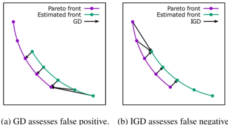
(a) GD assesses false positive. (b) IGD assesses false negative.
Figure 3: GD and IGD.
Performance Measures
To evaluate how accurately an estimated hyper-surface ap-proximates the Pareto front, we used the generational dis-tance (GD) (Veldhuizen 1999) and the inverted generational distance (IGD) (Zitzler et al. 2003):
GD(X, Y) := 1
|X|
X
x∈X
min
y∈Ykx−yk,
IGD(X, Y) := 1
|Y|
X
y∈Y
min
x∈Xkx−yk
whereXis a finite set of points sampled from an estimated hyper-surface andY is a validation set.
Figure 3 depicts what GD and IGD assess. These values can be viewed as the avarage length of arrows in each plot. Figure 3a implies that GD becomes high when the estimated front has a false positive area which is far from the Pareto front. Conversely, Figure 3b tells that IGD becomes high when the Pareto front has a false negative area which is not covered by the estimated front. Thus, we can say that the es-timated hyper-surface is close to the Pareto front if and only if both GD and IGD are small.
For the all-at-once fitting and the inductive skeleton fit-ting, we sampled the estimated B´ezier simplex as follows:
X :=
b(t)
t∈∆M−1, tm∈
0, 1
20, 2
20, . . . ,1 .
For the response surface method, we sampled the estimated response surface as follows:
X :={(x1, . . . , xM−1, r(x1, . . . , xM−1))
|x1, . . . , xM−1∈ {0,
1 20,
2
20, . . . ,1}},
where r(x1, . . . , xM−1) is an estimated polynomial func-tion. We repeated experiments 20 times5with different train-ing sets and computed the average and the standard devia-tions of their GDs and IGDs.
5
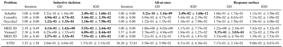
Table 1: GD and IGD (avg.±s.d. over 20 trials) with subsample size(1,3)for Schaffer, ConstrEx and Osyczka2;(1,2,1)for 3-MED, Viennet2 and 5-MED;(1,5,5)for S3TD. The best scores are shown in bold. (∗∗:p <0.05,∗:p <0.1)
Problem Inductive skeleton All-at-once Response surface
Iteration GD IGD Iteration GD IGD GD IGD
Schaffer 3.00±0.00 5.21e-10±1.16e-09 2.49e-02±1.68e-12 3.00±0.00 5.21e-10±1.16e-09 2.49e-02±1.68e-12 1.68e-01±1.74e-01 1.13e-01±3.50e-02 ConstrEx 3.00±0.00 4.94e-02±4.73e-02 5.44e-02±2.39e-02 3.00±0.00 4.94e-02±4.73e-02 5.44e-02±2.39e-02 5.09e-02±8.63e-03 7.13e-02±1.09e-02 Osyczka2 3.00±0.00 1.22e-01±1.35e-01 1.18e-01±7.98e-02 3.00±0.00 1.22e-01±1.35e-01 1.18e-01±7.98e-02 1.74e-01±1.56e-01 1.39e-01±4.08e-02
MED.3D 2.39±0.49 4.13e-01±1.42e+00 5.55e-02±2.44e-02 3.00±0.00 1.86e+00±6.02e+00 1.17e-01±7.75e-02 1.22e+00±2.10e-01 7.42e-02±5.22e-03 Viennet2 2.38±0.48 6.25e+00±1.37e+01 6.09e-02±8.44e-03 3.57±0.49 2.76e+05±4.94e+05 1.94e-01±1.27e-02 9.37e-01±3.03e-01 6.72e-02±2.59e-03 MED.5D 2.80±0.40 2.57e-01±3.33e-01 7.93e-02±1.05e-02 3.00±0.00 7.21e-01±4.12e-01 1.53e-01±1.87e-02 3.33e+00±6.76e-01 1.19e-01±7.53e-03
S3TD 3.25±1.58 2.04e-01±4.04e-02 1.37e-01±3.15e-02 36.20±33.81 5.58e-01±5.99e-01 6.31e-01±6.36e-01 7.17e-01±2.14e-01 9.88e-02±6.67e-03
Results
For each problem and method, the average and the stan-dard deviation of the GD and IGD are shown in Table 1. In Table 1, we highlighted the best score of GD and IGD out of all methods for each problem and added the results of Mann-Whitney’s one-tail U-test to check the best score was smaller than that of the other methods significantly. In case of conducting multiple tests, we corrected p-value by Holm’s method.
For B´ezier simplex fitting methods, the number of itera-tions until termination is also shown. The table shows that the fitting was finished in approximately three iterations in all cases except for the all-at-once fitting on S3TD.
Inductive skeleton vs. all-at-once For all the
two-objective problems, both methods obtained almost identical GD and IGD values. For three- and five-objective problems, the inductive skeleton fitting significantly outperformed the all-at-once fitting in both GD and IGD. Especially in Vien-net2, the all-at-once fitting exhibited unstable behavior in GD while the inductive skeleton fitting was stable.
Inductive skeleton vs. response surface The inductive
skeleton fitting achieved better IGDs in Schaffer, Osyczka2, 3-MED, and 5-MED but worse values in ConstrEx and Vi-ennet2. In terms of the average GD, the inductive skeleton fitting was better in all the problems except ConstrEx.
Discussion
In this section, we discuss approximation accuracy, required sample size, practicality for real-world data and objective map approximation of our method.
Approximation Accuracy
For three- and five-objective problems, the inductive skele-ton fitting achieved slightly better IGDs. The inductive skeleton fitting adjusts a small subset of control points at each step with already-adjusted control points of the faces. This reduces the number of parameters estimated at a time, which seems to prevent over-fitting.
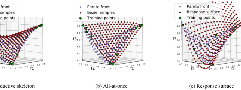
More significant differences can be seen in GD. Figure 4 shows the cause of these defferences: The all-at-once fitting obtained an overly-spreading B´ezier simplex while the in-ductive skeleton fitting found an exactly-spreading B´ezier simplex. Minimizing the squared loss (5) only imposes that
all sample points are close to the B´ezier simplex, which leads to a good IGD. However, it does not impose that all B´ezier simplex points are close to the sample points, which is needed to achieve a good GD. The inductive skeleton fit-ting stipulates that each face of the B´ezier simplex must be close to each face of the Pareto front (i.e., the Pareto front of each subproblem), which minimizes GD.
Similarly to the all-at-once fitting, the response surface has poor GDs. As we do not know the true Pareto set, it is difficult for grid sampling to obtain an exactly-spreading surface.
ConstrEx and Viennet2 are the only problems where the inductive skeleton fitting was worse than the response sur-face method. ConstrEx is a non-smooth curve that cannot be fitted by a single B´ezier curve (see Figure 1 in Appendix D). This type of Pareto fronts leads to a challenging problem: developing a method for gluing multiple B´ezier simplices to express a non-smooth surface. Viennet2 is a smooth surface but its curvature is severely sharp (see Figure 3 in Appendix D). Although Viennet2 is defined by quadratic functions (see Appendix B), its Pareto front cannot be fitted by the B´ezier simplex of degree three. This means that setting the degree of the B´ezier simplex grater than or equal to the maximum degree in the problem definition does not ensure approxima-tion accuracy. It would be useful to develop a way to un-derstand the required degree of the B´ezier simplex from the problem definition.
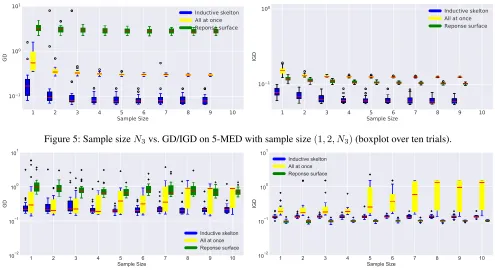
Required Sample Size
To achieve good accuracy, how many sample points does the B´ezier simplex require? Figure 5 shows transitions of GD and IGD on 5-MED when the sample size of each three-objective subproblem (two-dimensional face) variesN3 =
1, . . . ,10with fixedN1= 1andN2= 2. Surprisingly, both GD and IGD have already converged atN3= 4.
In case ofD = 3for 5-MED, which is a five-objective (M = 5) problem, the number of all control points to be esitimated is 3+55−1
(a) Inductive skeleton (b) All-at-once (c) Response surface
Figure 4: B´ezier triangles for 3-MED with sample size(1,2,1).
Practicality for Real-World Data
Now we discuss the practicality of the inductive skeleton fit-ting. Firstly, we focus on the performance of S3TD, which is a real-world problem. Table 1 indicates that the average IGD of the inductive skeleton fitting on S3TD was worse than that of the response surface method. However, the IGD itself is an order of10−1, which small in absolute sense consider-ing the number of the objective functions (M = 4) and the sample size of the validation set (N = 58) on S3TD. The average GD of the inductive skeleton method was smaller than that of the other methods and the difference was sig-nificant with significance level p = 0.1. Figure 6 shows transitions of GD and IGD on S3TD when the sample size of each three-objective subproblem (two-dimensional face) varies N3 = 1, . . . ,10 with fixedN1 = 1 andN2 = 5. We can observe that both GD and IGD already converged at
N3= 4as Figure 5. These results suggest that the inductive skeleton fitting can work properly in real-world problems.
In real-world problems, it seems to be difficult to know that the Pareto set/front is a simplex and in some cases, it is degenerated. However, a statistical test has been proposed to judge whether the Pareto set/front of a given problem is a simplex or not (Hamada and Goto 2018). This test tells us whether we can apply the inductive skeleton fitting to real-world problems. Furthermore, even if the Pareto front is de-generated, Theorem 1 states the Bezier simplex model can fit degenerate Pareto sets/fronts.
Objective Map Approximation
As well as the Pareto front approximation discussed and demonstrated so far, Theorem 1 ensures that our method can be used for approximating the Pareto set,X∗(f), and the restricted objective map, f : X∗(f) → fX∗(f). Such approximations may provide richer information about the problem. To check the performance of graph approximation, we made a sample of solution-objective pairs of 5-MED
X =
(x,f(x))∈R5×R5x∈X∗(f) and applied
the inductive skeleton fitting to it. Other settings were the same as the Pareto front approximation. Table 2 shows the GD and IGD values where the results of the all-at-once fit-ting are just for baseline. As the inductive skeleton fitfit-ting
achieved GD and IGD of10−1 order of magnitude, which means that it accurately approximates the graph of the re-stricted objective map in the abslute sense. In 5-MED, the graph of the restricted objective map on the Pareto set is a four-dimensional topological simplex in a 10-dimensional space. Although the codimension is six times higher than the case of Pareto front approximation, we have similar GD and IGD to ones of 5-MED in Table 1. This fact implies that the approximation error mainly depends on the intrinsic dimen-sionality rather than the ambient dimendimen-sionality.
Conclusions
In this paper, we have proposed the B´ezier simplex model and its fitting algorithm for approximating Pareto fronts of multi-objective optimization problems. An approximation theorem of the B´ezier simplex has been proven. Numeri-cal experiments have shown that our fitting algorithm, the inductive skeleton fitting, obtains exactly-spreading B´ezier simplices over synthetic Pareto fronts of different shape and dimensionality. It has been also observed that a real-world problem with four objectives but only 58 points is accurately fitted. The proposed model and its fitting algorithm drasti-cally reduce the sample size required to describe the entire Pareto front.
The current algorithm has some drawbacks. The inductive skeleton fitting requires that each subproblem must have a non-empty sample, which may be too demanding for some practice. Furthermore, the loss function for fitting does not take into account of the sampling error of the Pareto front. To get a more stable approximation under wild samples, we plan to extend the (deterministic) Bezier simplex to a prob-abilistic model.
Figure 5: Sample sizeN3vs. GD/IGD on 5-MED with sample size(1,2, N3)(boxplot over ten trials).
Figure 6: Sample sizeN3vs. GD/IGD on S3TD with sample size(1,5, N3)(boxplot over ten trials).
Table 2: GD and IGD (avg.±s.d. over 20 trials) with sample size(1,2,1)for the graph of 5-MED.
Inductive skeleton All-at-once
Iteration GD IGD Iteration GD IGD
2.85±0.36 3.35e-01±9.27e-02 2.05e-01±3.37e-02 3.00±0.00 1.34e+00±1.95e+00 2.79e-01±8.00e-02
Acknowledgements
We wish to thank Dr. Yuichi Ike for checking the proof and making a number of valuable suggestions.
References
Borges, C. F., and Pastva, T. 2002. Total least squares fitting of B´ezier and B-spline curves to ordered data. Computer Aided Geometric Design19(4):275–289.
Chand, S., and Wagner, M. 2015. Evolutionary many-objective optimization: A quick-start guide. Surveys in Op-erations Research and Management Science20(2):35–42. Chiba, K.; Makino, Y.; and Takatoya, T. 2009. Design-informatics approach for intimate configuration of silent su-personic technology demonstrator. In Proceedings of the 47th AIAA Aerospace Sciences Meeting. Orlando, Florida, USA: American Institute of Aeronautics and Astronautics.
Coello, C. A. C.; Lamont, G. B.; and Van Veldhuisen, D. A. 2007. Evolutionary Algorithms for Solving Multi-Objective Problems. Genetic and Evolutionary Computation Series. Springer Science+Business Media, LLC.
Deb, K., and Srinivasan, A. 2006. Innovization: Innovat-ing design principles through optimization. InProceedings of the 8th Annual Conference on Genetic and
Evolution-ary Computation, GECCO ’06, 1629–1636. New York, NY, USA: ACM.
Farin, G. 2002.Curves and Surfaces for CAGD: A Practical Guide. Computer graphics and geometric modeling. Morgan Kaufmann.
Gelman, A., and Hill, J. 2007. Data Analysis Using Regres-sion and Multilevel/Hierarchical Models. Analytical Meth-ods for Social Research. Cambridge University Press.
Gelman, A.; Carlin, J.; Stern, H.; Dunson, D.; Vehtari, A.; and Rubin, D. 2013.Bayesian Data Analysis, Third Edition. Chapman & Hall/CRC Texts in Statistical Science. Taylor & Francis.
Goel, T.; Vaidyanathan, R.; Haftka, R. T.; Shyy, W.; Queipo, N. V.; and Tucker, K. 2007. Response surface approxima-tion of Pareto optimal front in multi-objective optimizaapproxima-tion.
Computer Methods in Applied Mechanics and Engineering
196(4):879–893.
Hamada, N., and Goto, K. 2018. Data-driven analysis of Pareto set topology. InProceedings of the Genetic and Evo-lutionary Computation Conference, GECCO ’18, 657–664. New York, NY, USA: ACM.
optimization framework taking account of spread and even-ness of approximate solutions. InProceedings of the 2010 IEEE Congress on Evolutionary Computation, CEC 2010, 787–794.
Kuhn, H. W. 1967. On a pair of dual nonlinear programs.
Nonlinear Programming1:38–45.
Li, B.; Li, J.; Tang, K.; and Yao, X. 2015. Many-objective evolutionary algorithms: A survey.ACM Computing Surveys
48(1):13:1–13:35.
Lovison, A., and Pecci, F. 2014. Hierarchical stratifica-tion of Pareto sets.ArXiv e-prints. http://arxiv.org/abs/1407. 1755.
Mastroddi, F., and Gemma, S. 2013. Analysis of Pareto fron-tiers for multidisciplinary design optimization of aircraft.
Aerospace Science and Technology28(1):40–55.
Nebro, A.; Durillo, J.; and Vergne, M. 2015. Redesign-ing the jMetal multi-objective optimization framework. In
Proceedings of the Companion Publication of the 2015 An-nual Conference on Genetic and Evolutionary Computation, GECCO Companion ’15, 1093–1100. New York, NY, USA: ACM.
Obayashi, S.; Jeong, S.; and Chiba, K. 2005. Multi-objective design exploration for aerodynamic configurations. In Pro-ceedings of the 35th AIAA Fluid Dynamics Conference and Exhibit. Toronto, Ontario, Canada: American Institute of Aeronautics and Astronautics.
Rodr´ıguez-Ch´ıa, A. M., and Puerto, J. 2002. Geometri-cal description of the weakly efficient solution set for mul-ticriteria location problems.Annals of Operations Research
111:181–196.
Shao, L., and Zhou, H. 1996. Curve fitting with B´ezier cubics.Graphical Models and Image Processing58(3):223– 232.
Shoval, O.; Sheftel, H.; Shinar, G.; Hart, Y.; Ramote, O.; Mayo, A.; Dekel, E.; Kavanagh, K.; and Alon, U. 2012. Evolutionary trade-offs, Pareto optimality, and the geometry of phenotype space.Science336(6085):1157–1160. Smale, S. 1973. Global analysis and economics I: Pareto optimum and a generalization of Morse theory. In Peixoto, M. M., ed.,Dynamical Systems. Academic Press. 531–544. Veldhuizen, D. A. V. 1999.Multiobjective Evolutionary Al-gorithms: Classifications, Analyses, and New Innovations. Ph.D. Dissertation, Department of Electrical and Computer Engineering, Graduate School of Engineering, Air Force In-stitute of Technology, Wright-Patterson AFB, Ohio, USA. Vrugt, J. A.; Gupta, H. V.; Bastidas, L. A.; Bouten, W.; and Sorooshian, S. 2003. Effective and efficient algorithm for multiobjective optimization of hydrologic models. Water Resources Research39(8):1214–1232.