Solution of bang - bang optimal control problems by using bezier
polynomials
Ayat Ollah Yari*
Department of Applied Mathematics, Faculty of Mathematical Sciences,
Payame Noor University, PO BOX 19395-3697, Tehran, Iran. E-mail: a [email protected]
Mirkamal Mirnia
Department of Applied Mathematics, Faculty of Mathematical Sciences, University of Tabriz.
E-mail: [email protected]
Aghileh Heydari
Department of Applied Mathematics, Faculty of Mathematical Sciences,
Payame Noor University, PO BOX 19395-3697, Tehran,Iran. E-mail: a [email protected]
Abstract In this paper, a new numerical method is presented for solving the optimal control problems of bang-bang type with free or fixed terminal time. The method is based on Bezier polynomials which are presented in any interval as [t0, tf]. The problems are reduced to a constrained problems which can be solved by using Lagrangian method. The constraints of these problems are terminal state and conditions. Illustrative examples are included to demonstrate the validity and applicability of the method.
Keywords. Optimal control, Bang-Bang control, Minimum-time, Bezier polynomialsfamily, Best
approx-imation.
2010 Mathematics Subject Classification. 49N10, 49M37, 65D07.
1. Introduction
Bang-bang control switching between upper and lower bounds, is the optimal strat-egy for solving a wide variety of control problems. The control of a dynamical system has lower and upper bounds and the system model is linear in the input and nonsin-gular. Bang-bang control is often the appropriate choice because of the nature of the actuator of the physical system.
Switching from one mode of the system to another one can be modelled by a bang-bang type control. Bang-bang-bang type controls arise in well-known application areas such as robotics, rocket flights , cranes, and also in applied physics [1, 2]. There are a large number of research papers that employ this method to solve optimal control problems (see for example [5,6,10,11,12,13,14,15,16,25,26,27] and the references
Received: 25 January 2016 ; Accepted: 4 May 2016.
∗Corresponding author.
therein).
In this paper, a numerical method is presented to solve a class of bang-bang con-strained optimal control problems, where the focus is on time-optimal control. First the optimal control problem is reduced to constrianed problems with equal constraint defined by the terminal state in time space. Also a computational method is pre-sented for solving linear constrained quadratic optimal control problems by using Bezier polynomials. The method is based on approximating the state and the con-trol variables with Bezier polynomials. Our method consists of reducing the optimal control problem to an NLP one by first expanding the state rate ˙x(t) as a Bezier polynomial expansion with unknown coefficients and the control u(t) as the bang-bang control. The operational matrix of differentiation DΦ is obtained in order to
approximate the differential part of the problem. The paper is organized as follows: In Section 2, we describe the basic formulation of the Bezier functions required for our subsequent development. Section 3 is devoted to the formulation of bang-bang optimal control problems. Section 4 summarizes the application of this method to the optimal control problems, and in Section 5 we report our numerical result along with showing the accuracy of the proposed method.
2. Some properties of bernstein and bezier polynomials on[t0, tf]
The Bernstein basis polynomials of degreenon [t0, tf] are defined as
Bi,n(t) = (
n i )
(t−t0)i(tf−t)n−i, i∈[0, n], (2.1)
whereiis integer number and the binomial coefficients are given by
( n
i )
=
n!
i!(n−i)!, i∈[0, n],
0, elsewhere.
Some properties of these polynomials are
(i)Bi,n(t0) =δi,0(tf−t0)n and Bi,n(tf) =δi,n(tf−t0)n , whereδ is the Kronecker
delta function.
(ii)Bi,n(t) has two roots, with multiplicitiesiatt=t0 andn−iat t=tf.
(iii)Bi,n(t)≥0 fort∈[t0, tf] andBi,n(tf−t) =Bn−i,n(t−t0).
(iv) The Bernstein polynomials form a partition of unity i.e.∑ni=0Bi,n(t) = (tf−t0)n.
(v) Recursion: Bi,n(t) = (tf−t)Bi,n−1(t) + (t−t0)Bi−1,n−1(t).
(vi) Derivative: dBi,n(t)
dt =
1
tf−t0[(n+1−i)Bi−1,n(t)+(2i−n)Bi,n(t)−(i+1)Bi+1,n(t)].
2.1. Definition of bezier polynomials on [t0,tf]. We will express Bezier
(poly-nomials) curves in terms of Bernstein polynomials, defined explicitly by
pn(t) = n ∑
i=0
whereci=c[t<n0 −i>, t<i>f ] named control points or Bezier pionts and t<n0 −i> means thatt0appearsn−itimes. For example,c[t<03>, t<f0>] =c[t0, t0, t0]. Some properties
of Bezier polynomials on [t0, tf] are
(i) Symmetry: ∑ni=0ciBi,n(t−t0) = ∑n
i=0cn−iBi,n(tf−t).
(ii) Linear precision: 1 (tf−t0)n−1
∑n i=0
i
nBi,n(t) =t−t0.
2.2. The operational matrix of the bezier polynomials. Consider
Φn(t) = [B0,n(t), B1,n(t), ..., Bn,n(t)]T, t∈[t0, tf], (2.3)
whereT denotes transposition.
2.3. The operational matrix of derivative. The differentiation of vector Φn(t)
can be expressed as
Φ′n(t) =DΦΦn(t), (2.4)
whereDΦis the (n+ 1)(n+ 1) operational matrix of derivative for the Bezier
poly-nomialsBi,n(t) whicht∈[t0, tf] and satisfies in
DΦ=
1
tf−t0
Dϕ, (2.5)
whereDϕis the (n+ 1)(n+ 1) operational matrix of derivative for Bezier polynomials Bi,n(u) whichu∈[0,1] andi= 0, ..., n.
2.4. Function approximation. Suppose that H = L2[t
0, tf] is a Hilbert space
with the inner product defined as < f.g > = ∫tf
t0 f(t)g(t)dt and because the set
{B0,n(t), B1,n(t), ..., Bn,n(t)} is a complete basis in Hilbert spaceH then, any
poly-nomialB(t) of degree n can be expanded in terms of Bi,n(t), i= 0, . . . , nas follows
B(t) =
n ∑
i=0
ciBi,n(t). (2.6)
Also Φn(t)⊂H is the set of Bezier polynomials of degreen. LetSn=span {Φn(t)} and f be an arbitrary element in H. Since Sn is a finite dimensional and
closed subspace, thereforeSn is a complete subset of H. So, f has the unique best approximation out ofSn such asS0 ̸∈Sn. So, there exist the unique coefficients ci,
i=0,. . . , n such that [16] any functionf ∈H can be approximated in terms of Bezier polynomials as
f(t)≃S0= n ∑
i=0
ciBi,n(t) =CTΦn(t), (2.7)
whereC= [c0, . . . , cn]T can be obtained as
CT <Φn.Φn>=< f.Φn>= ∫ tf
t0
f(t)Φn(t)dt
LetR=<Φn.Φn>be (n+ 1)×(n+ 1) matrix called the dual matrix of Φn(t), which
can be determined by
Ri+1,j+1=< Bi,n.Bj,n>= ∫ tf
t0
Bi,n(t)Bj,n(t)dt
= (tf−t0)2n+1 (n
i )(n
j )
(2n+ 1)(i2+nj), (2.9)
wherei, j= 0, . . . , n. We explain and prove the folowing lemma from [18].
Lemma 2.1. Suppose that the function f : [t0, tf] → R be n+ 1 times
continu-ously differentiable (i.e.f ∈ Cn+1[t
0, tf]), and Sn=span{Φn(t)}. If CTB is the best
approximation off out ofSn, then
|f−CTB|L2[t0,tf]≤
ˆ
K
(n+ 1)!
√
t2fm+3−t20n+3
2n+ 3 , (2.10)
whereKˆ=max|f(n+1)(t)|, t∈[t0, tf].
Proof. We know that {1, x, x2, ..., xn} is a basis for polynomials space of degree
≤n. Therefore we define y1(x) =f(t0) +xf′(t0) +x
2
2!f′′(t0) +...+ xn
n!f (n)(t
0). By
the Taylor expansion we have
|f(x)−y1(x)|=|f(n+1)(ξx) xn+1
(n+ 1)!|, (2.11)
whereξx∈(t0, tf). SincecTBis the best approximation of f out ofSn. Theny1∈Sn
and from Eq. (2.11) we have
∥f−cTB∥2L2[t0,tf] ≤ ∥f−y1∥2L2[t0,tf]
=
∫ tf
t0
|f(x)−y1(x)|2dx
=
∫ tf
t0
|f(n+1)(ξx)|2( x
n+1
(n+ 1)!)
2dx
≤( ˆ
K
(n+ 1)!)
2 ∫ tf
t0
x2n+2dx
= ( ˆ
K
(n+ 1)!)
2(t 2n+3
f −t
2n+3 0
2n+ 3 )
= ( ˆ
K
(n+ 1)!)
2(t 2n+3 f (1−(
t0
tf)
2n+3)
2n+ 3 )
∼
= ( ˆ
Ktn f
(n+ 1)!)
2( t 3 f
Then by taking square roots, the proof is complete. We can rewrite Eq. (2.10) as following
|f−CTB|L2[t 0,tf]≤
ˆ
K
(n+ 1)!
√
t2fm+3−t20n+3
2n+ 3
∼
= ˆ
K
(n+ 1)!
√
(t2fn+3(1−(t0
tf)
2n+3)
2n+ 3
)
∼
= ˆ
Ktn f
(n+ 1)!
√ t3
f
2n+ 3. (2.12)
This Lemma shows that the error vanishes asn→ ∞.
3. Optimal control problems of bang-bang type
Optimal control problems of bang-bang type are problems where control function includes an uncontinuse point and the control on the environment of that point only has minimize and maximize amount. Now we considere optimal control problems of bang-bang type with normalized constraint| u|≤ 1. If a switching point exists, then control sequence will be as{−1,1}or{1,−1}. For better perception, considere equations system as following
˙
x(t) =Ax(t) +Bu(t). (3.1)
If we want this system arrive from primary statex0 to terminal statex1 in the least
time, in a case that trajectory state and control are optimal. Hamiltonian function is obtained for (4.1) using pontryagin maximum principle on two domain space as following
H=−1 +λ1x˙1+λ2x˙2+ (b1λ1+b2λ2)u, (3.2)
where B = [b1, b2]T. Because H is linear base u, thus for making maximum of H ,
we should haveu= 1 oru=−1. Because chosing these amounts are dependant on the sign of fourth coefficient on H , thus only controls that can led to minimizing transfering time are as following
u∗=sgn(b1λ1+b2λ2). (3.3)
This control is scrap constant that its discontinuity points will be on the zero places of following function
S=b1λ1+b2λ2, (3.4)
Lemma 3.1. a: If eigenvalues ofAare real, then switching function has at most one root.
b: In this state a sequence of controls which are optimal are as following:
{1},{−1},{−1,1},{1,−1}.
singular controls. Becuase in some problems, switching function S is zero for all
amounts oftthatt1≤t≤t2, thus control amountsuis not obtinated fromu=sgn(S)
that in this case control function is called singular and becuase singular controls always aren’t optimal, thus we search for unsingular controls that are exclusively optimal .For example in the fuel optimal control problems the fuel is used for guidance of vehicles from primal piont to final piont, that we want this used fuel be arrived to the least amount. It seems logical that consumable fuel amount on the base of time, will be multiplety of bigness forse of conveying. Therefore consumable fuel will equal with
|u|. In this case only unsingular controls are as following
{−1,0,1},{0,1},{1},{1,0,−1},{0,−1},{−1}.
4. Problem statement
Consider the nonlinear system
˙
x(t) =A(t)x(t) +B(t)u(t), (4.1)
x(t0) =x0, x(tf) =x1, (4.2)
u(t)∈[a, b], (4.3)
where t∈[t0, tf], tf is the terminal time free or fixed, A(t) = (ai,j(t))n×n , B(t) =
(bi,j(t))m×m are matrices,x(t) isn×1 state vector, the control u: [t0, tf] →[a, b],
˙
x(t) :Rn×[a, b]→ Rn is smooth in xexcept at the time points where the control uswitches between a and b. The problem is to find the switching points u(t) and the corresponding state trajectory x(t) satisfying Eqs. (4.1), (4.2) and (4.3) while minimizing (or maximizing) the quadratic performance index
Z= 1 2x
T(tf)Gx(tf) +1
2
∫ tf
t0
(xT(t)Q(t)x(t) +uT(t)R(t)u(t))dt, (4.4)
where G(t) = (gi,j(t))n×n, Q(t) = (qi,j(t))n×n are symmetric positive semi-definite
matrices and andR(t) = (ri,j(t))m×m is a symmetric positive definite matrix.
4.1. Variational problems. Consider the variational problem
Z(x(t)) =
∫ tf
t0
F(t, x(t),x˙(t), . . ., x(n)(t))dt, (4.5)
with the boundary conditions as
x(t0) =a0, x˙(t0) =a1, . . ., x(n−1)(t0) =an−1, (4.6)
x(tf) =b0, x˙(tf) =b1, . . ., x(n−1)(tf) =bn−1, (4.7)
wherex(t) = [x1(t), x2(t), . . . , xn(t)]T. The problem is to find the extremum of (4.5),
variational problem into a set of algebraic equations by first expandingx(t) in terms of Bezier polynomials with unknown coefficients.
5. The proposed method
Let
t∈[tj, tj+1], (5.1)
xji(t)≃Φnj(t)TXij, (5.2)
u∗(t) =uj, (5.3)
whereXij, i= 1, . . . , n, are state coefficient vectors on [tj, tj+1] trajectory. Then by
using Eq. (2.4) we get
˙
xji(t)≃[DjΦΦjn(t)]TXi. (5.4)
By using Eqs. (5.1) and (5.3) we will have
xj(t)≃[Φjn(t)TXj]T = [
n ∑
r=0
Br,nj (t)X1jr, . . . , n ∑
r=0
Br,nj (t)Xnrj ]T, (5.5)
whereXj= (Xirj)n×(n+1)is the state coefficient matrix. The boundary conditionsin
Eq. (4.2) can be rewritten as
x1(t0) =x10=d 1 0⊗EΦ
1
n(t), (5.6)
xm(tf) =xm1 =d1m⊗EΦ1n(t), (5.7)
DjΦ= 1
tj+1−tj
Dϕ, (5.8)
where tm =tf, d10 andd1m are n×1 constant vectors, E = [1, . . . ,1] is 1×(n+ 1)
constant vector, and the symbol ⊗denotes the Kronecker product [33]. If x1(t 0) or xm(tf) are unknown in Eq. (4.2), then we put
x1(t0)≃[Φ1n(t0)TX1]T = [ n ∑
r=0
B1r,n(t0)X11r, . . . , n ∑
r=0
B1r,n(t0)Xnr1 ]
T, (5.9)
xm(tf)≃[ΦnT(tf)Xm]T = [ n ∑
r=0
Br,nm(tf)X1mr, . . . , n ∑
r=0
Bmr,n(tf)Xnrm]
T. (5.10)
5.1. Performance index approximation. By substituting Eqs. (5.6), (5.7) and
(5.8) into Eq (4.5) we get
min(max)Zj= 1 2x
jT 1 G
j 1x
j 1+
1 2X
jT[ ∫ tj+1
tj
Φjn T
(t)Qj(t)Φjn(t)dt]Xj
+u
2 j
2 [
∫ tj+1
tj
Let
Pxj =
∫ tj+1
tj
ΦjTn (t)Qj(t)Φjn(t)dt, and Puj=
∫ tj+1
tj
Rj(t)dt. (5.12)
By substituting Eq (5.12) in Eq (5.11) we get
Zj=Z[Xj, uj] = 1 2X
jT
( ˆPj+Pxj)X j
+1 2u
2 jP
j
u, (5.13)
where ˆPj= (ΦjT n G
j 1Φ
j
n)(tj+1).andx j 0=x
j(t j), x
j 1=x
j(t j+1).
The boundary conditions in Eq. (4.2) can be expressed as
q01=x 1
(t0)−x10, q 1 0= (q
1
0i), i= 1, . . . , n, (5.14) q1m=xm(tf)−xm0, q1m= (q0mi), i= 1, . . . , n. (5.15)
We now find the extremum of Eq. (5.12) subject to Eqs. (5.13) and (5.14) by using the Lagrange multiplier method. Let
Z[Xj, uj, λj0, λj1] =Z[Xj, uj] +λj0Qj0+λj1Qj1, (5.16)
where Qj0 = (q0ji), i = 1, . . . , n and Qj1 = (qj1i), i = 1, . . . , n are (n×1) constant vectors. The necessary condition for the extremum of Eq. (5.16) is
∇Z[Xj, uj, λ j 0, λ
j
1] = 0. (5.17)
Finally we have subject function as folloving
min(max)Z=min(max)Z1+· · ·+min(max)Zm. (5.18)
We now use necessary conditions to find switching points as following
xj−1(tj) =xj(tj), j= 1, . . . , m, (5.19)
conditions in Eq. (5.19), can be expressed as
dj =xj−1(tj)−xj(tj) = 0, j= 1, . . . , m, (5.20)
dj= (dji), i= 1, . . . , n, j= 1, . . . , m. (5.21)
Now we find switching points by solving Eqs. (5.19) and (5.20) which is nonlinear system.
5.2. Performance index approximation for the variational problem. Now we
want to extensionx(n)(t) in terms of the Bezier polynomials. So let
x(t) =XTΦn(t), (5.22)
whereXT is vector of order 1×(n+ 1), By derivating Eq. (5.22) with respect totwe
get
x(1)(t) =XTDΦΦn(t), (5.23)
where DΦ is operational matrix of derivative given in Eq. (2.5). By n derivaton of
(5.22) with respect tot we have
By extending (t−t0)i, i= 0,1, . . . , n−1 in terms of Bezier polynomials as
(t−t0)i=diΦn(t), i= 0,1, . . . , n−1, (5.25)
wheredi, i= 0,1, . . . , n−1,are constant vectors of order 1×(n+ 1) given by
di= (n 1
i )
(tf−t0)n−i
[0, . . . , (
i i )
, (
i+ 1
i )
, . . . , (
n i )
], i= 0,1, . . . , n−1, (5.26)
So Eq. (4.5) can be rewritten as
Z[x(t)] =Z[X]. (5.27)
The boundary conditions in Eqs. (4.6) and (4.7) can be expressed as
rk0=x(k)(a)−ak= 0, k= 0, . . . , n−1, (5.28)
rk1=x(k)(b)−bk= 0, k= 0, . . . , n−1. (5.29)
We now find the extremum of Eq. (4.5) subject to Eqs. (5.28) and (5.29) by using the Lagrange multiplier method. Let
Z[x, λ] =Z[x, λ0, λ1] +λ0R0+λ1R1, (5.30)
where R0 = (r0
k), k = 1, . . . , n and R
1 = (r1
k), k = 1, . . . , n are (n×1) constant
vectors. The necessary conditions for the extremum of Eq. (5.30) are
∇Z[X, λ0, λ1] = 0. (5.31)
6. Illustrative examples
This section is devoted to numerical examples. We implemented the proposed method in last section with MATLAB (2012). To illustrate our method, we present four numerical examples, and make a comparison with some of the results in the lit-eratures.
Example 1. This example is adapted from [17]
minZ =
∫ 5
0
|u(t)|dt, (6.1)
subject to
˙
x1(t) =x2(t)−u(t), (6.2)
˙
x2(t) =u(t), (6.3)
|u(t)| ≤1, (6.4)
with the boundary conditions as
x1(0) =
1
2, x2(0) = 1, (6.5)
Here we solve this problem with Bezier polynomials by choosingn= 2. Let
x1(t) = ΦT2(t)X1, (6.7)
x2(t) = ΦT2(t)X2, (6.8)
u(t) =
−1, [0, t1],
0, [t1, t2],
1, [t2,5],
(6.9)
(6.10)
where
X1= [X10, X 1 1, X
2 1]
T, X
2= [X20, X 1 2, X
2 2]
T. (6.11)
By using Eqs. (5.16)-(5.18) and Eqs. (6.5)-(6.11) for j=1 and considering interval [0, t1] we obtain
t1= 3− √
2, X1
1 = [ 1155 5809,
248 299,
1153 1201],
X21= [11212819, 197 2392,−
577 2477],
x1 1(t) =
1155
5809B0,2(t) + 2248299B1,2(t) +11531201B2,2(t) =−12t
2+ 2t+1 2,
x12(t) =11212819B0,2(t) + 2 197
2392B1,2(t)− 577
2477B2,2(t) =−t+ 1, Z1=t1= 3−
√
2,
which is exact solution. Forj=2 and considering interval [t1, t2] we obtain
t2= 3 + √
2, X2
1 = [ 1138 3771,
357 1801,
119 1257],
X22= [−1393102,− 102 1393,−
102 1393],
x2 1(t) =
1138
3771B0,2(t) + 2 357
1801B1,2(t) + 119
1257B2,2(t) =
1
36028797018963968t 2−577
985t+ 3975 1189,
x22(t) =−1393102B0,2(t)−2 102
1393B1,2(t)− 102
1393B2,2(t) =− 577 985, Z2= 0.
Where the exact solution as following
x2∗ 1 (t) = (
√
2−2)t+ 9−4√2 =−577985t+39751189, x2∗
2 (t) = 1−t1= √
2−2 =−577985.
Forj=3 and considering interval [t2,5] we obtain
t2= 3 + √
2, X13= [2174985,11891393,0],
X3 2 = [−
985 577 ,−
1189 1393 ,0],
x31(t) =2174985B0,2(t) + 211891393B1,2(t) = 12t2−6t+352,
x3
2(t) =−− 985
577 B0,2(t)−2 1189
1393B1,2(t) =t−5, Z3= 5−t2= 2−
√
Figure 1. Plot of state optimal trajectory with bang-bang control for example 1
Finally value of object function isZ=Z1+Z2+Z3= 5−2 √
2.
Example 2. This example is adapted from [17]
minZ =
∫ tf
0
(|4 +u(t)|)dt, (6.12)
subject to
˙
x1(t) =x2(t), (6.13)
˙
x2(t) =u(t), (6.14)
|u(t)| ≤1. (6.15)
with the boundery conditions as
x1(0) =
1
2, x2(0) = 0, (6.16)
x1(tf) =−
1
2, x2(tf) = 0. (6.17)
Here we solve this problem with Bezier polynomials by choosingn= 2. Let
u(t) =
−1, [0, t1],
0, [t1, t2],
1, [t2, tf].
(6.18)
By using Eqs. (6.7) , (6.8) and (6.11) forj=1 and considering interval [0, t1] we obtain
t1=
√
6 3 , X11= [34,
3 4,
1 4],
X1 2 = [0,−
1079 1762 ,−
x1
1(t) = 34B0,2(t) + 2 3
4B1,2(t) + 1
4B2,2(t) =− 1 2t
2+1 2,
x1
2(t) =−2 1079
1762B1,2(t)− 1079
881B2,2(t) =−t,
Z1= 5t1= 5
√
6 3 ,
which is exact silution. Forj=2 and considering interval [t1, t2] we obtain
t2=
√
6 2 , X2
1 = [1,11258999068426241 ,−1],
X22= [−9804801,−9804801,−9804801],
x2
1(t) =B0,2(t) + 211258999068426241 B1,2(t)−B2,2(t) =−5629499534213121 t2−
√
6 3 t+
5 6,
x2
2(t) =−4801980B0,2(t)−2 4801
980B1,2(t)− 4801
980B2,2(t) =−
√
6 3 ,
Z2= 4(
√
6 2 −
√
6 3 ).
Where the exact solution as following
x2∗ 1 (t) =−
√
6 3 t+
5 6, x2∗
2 (t) =−t1=−
√
6 3 .
Forj=3 and considering interval [t2, t3] we obtain
tf =t3,
t3=t1+t2= 5
√
6 6 , X13= [−41,−
3 4 ,−
3 4 ], X3
2 = [− 1079 881 ,−
1079 1762 ,0], x3
1(t) =− 1
4B0,2(t)−2 3
4B1,2(t)− 3
4B2,2(t) = 1 2t
2−5√6 6 t+
19 12, x3
2(t) =− 1079
881B0,2(t)−2 1079
1762B1,2(t) =t−5
√
6 6 , Z3= 5(t3−t2) = 5
√
6 3 , Z =Z1+Z2+Z3= 4
√
6,
whichZ is finally value of object function.
Note that all approximation solutions of example 1 and example 2 are computed with decimal number 16 on intervals [0,5] and [0, t3] respectively. Also if you consider
another kind of value for control except above value, there is no solution for or if the soluotion exists it would be negative for switching points.
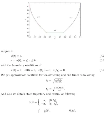
Example 3. To illustrate some of the basic concepts involved when controls are
bounded and allowed to have discontinuities we start with a simple physical problem: Derive a controller such that a car moves a distance with a minimum time[22]. The motion equation of the car is as folowing:
minZ =
∫ tf
0
Figure 2. Plot of state optimal trajectory with bang-bang control for example 2
subject to
¨
x(t) =u, (6.20)
u=u(t), a≤u≤b, (6.21)
with the boundary conditions of
x(0) = 0, x˙(0) = 0, x(tf) =c, x˙(tf) = 0. (6.22)
We get approximate solutions for the switching and end times as following
t1= √
2ac b(a+b),
tf =
√ 2c(a+b)
ab .
And also we obtain state trejectory and control as folowing
u(t) =
{
b, [0, t1], −a, [t1, tf],
x(t) =
1 2bt
2, [0, t
1],
−1
2a(t−tf)
2+c, [t 1, tf],
which is the exact solution. It is observed that the state trajectory is depended onb
anda, c, tf respectively in intervals [0, t1] and [t1, tf].
7. Conclusion
but the end point ofx(t) is known, u(t) is bounded between a and b. Several test problems were used to see the applicability and efficiency of the method. The ob-tained results show that the new approach can solve the problem effectively. It was investigated to solve bang-bang optimal control problems with a nonlinear constraint.
References
[1] J. H. R. Kim, H. Maurer, Y. A. Astrov, and M. Bode,High speed switch-on of a semiconduc-tor gas discharge image converter using optimal control methods, Journal of Computational Physics,170(1)(2001),395-414.
[2] C. Yalcin Kaya Stephen, K. Lucas and Sergey, and T. Simakov,Computations for Bang Bang Constrained Optimal Control Using a Mathematical Programming Formulation, Optimal Con-trol Applications and Methods,1(2002),1-14.
[3] G. J. Olsder, An open- and closed-loop bang-bang control in nonzero-sum differential games, SIAM Journal on Control and Optimization,40(4)(2001), 1087-1106 .
[4] S. A. Dadebo, K. B. McAuley, and P. J. McLellan,On the computation of optimal singular and bang-bang controls, Optimal Control Applications and Methods,19(1998) ,287-297 .
[5] M. Gachpazan, Solving of time Varying quadratic optimal control problems by using Bezier control points, Computational and Applied Mathematics,2(2011), 367-79.
[6] Y. Ordokhani, and S. Davaeifar,Approximate Solutions of Differential Equations by Using the Bernstein Polynomials, International Scholarly Research Network ISRN Applied Mathematics, Article ID 787694, 15 pages,2011.
[7] R. R. Mohler,Bilinear Control Processes, Academic Press, New York, Chap. 3, 1973.
[8] R. R. Mohler,Nonlinear Systems, V.2 Applications to Bilinear Control, Prentice Hall, Englewood Cliffs, NJ, Chap. 7,1991,
[9] E. B. Meier, and A. E. Bryson Jr, Eiffcient algorithm for time optimal control of a two-link manipulator, Journal of Guidance, Control and Dynamics,13(1990), 859-866 .
[10] F. Ghomanjani, and M. Hadifarahi,Optimal control of switched systems based on Bezier control points, I. J. Intelligent Systems and Appications,7(2012), 16-22.
[11] G. S. C. J. Hu, Ong, and C. L. Teo,An enhanced transcribing scheme for the numerical solution of a class of optimal control problems, Engineering Optimization,34(2)(2002), 155-173 . [12] R. Bertrand, and R. Epenoy,New smoothing techniques for solving bang-bang optimal control
problems— numerical results and statistical interpretation, Optimal Control Applications and Methods,23(2002),171-197 .
[13] C. Y. Kaya, and J. L. Noakes,Computational method for time-optimal switching control, Journal of Optimization Theory and Applications,117(1)(2003).
[14] S. T. Simakov, C. Y. Kaya, and S. K. Lucas,Computations for time-optimal bang-bang control using a Lagrangian formulation, Preprints of IFAC 15th Triennial World Congress, Barcelona, Spain 2002.
[15] Z. Foroozandeh, and M. Shamsi,Solution of nonlinear optimal control problems by the inter-polating scaling functions, Acta Astronautica,72(2012), 21-6.
[16] E. Kreyszig,Introduction Functional Analysis with Applications, John Wiley and Sons Incor-porated,1978.
[17] Pinch, R. Eind, Optimal Control and the Calculus of Variations,1993.
[18] M. Alipour, and D. Rostamy,Bernstein polynomials for solving Abels integral equation, The Journal of Mathematics and Computer Science,3(4)(2011),403-12.
[19] H. Jaddu, E. Shimemura,Computation of optimal control trajectories using Chebyshev polyno-mials parameterization and quadratic programming, Optimal Control Appl. Methods,20(1999), 21-42.
[23] S. Dixit, V. K. Singh, A. K. Singh, and O. P. Singh, Bernstein direct method for solving variational problems, International Mathematical Forum,5(48)(2010), 2351-70.
[24] M. Razzaghi , and G. Elnagar,Linear quadratic optimal control problems via shifted Legendre state parameterization, Internat J. Systems Sci.,25(1994), 393-99.
[25] H. R. Marzban, and M. Razzaghi,Hybrid functions approach for linearly constrained quadratic optimal control problems, Appl Math. Modell,27(2003), 471-85.
[26] H. R. Marzban, and M. Razzaghi,Rationalized Haar approach for nonlinear constrined optimal control problems, Appl Math. Modell,34(2010), 174-83.
[27] S. Mashayekhi, Y. Ordokhani, and M. Razzaghi,Hybrid functions approach for nonlinear con-strained optimal control problems, Commun Nonlinear Sci Numer Simulat.17(2012), 1831-43. [28] C. H. Hsiao, Haar wavelet direct method for solving variational problems, Mathematics and
Computers in Simulation,64(2004), 569-85.
[29] R. K. Mehra, and R. E. Davis,A generalized gradient method for optimal control problems with inequality constraints and singular arcs, IEEE Trans Automat Contr.,17(1972), 69-72. [30] M. J. D. Powell,An efficient method for finding the minimum of a function of several variables
without calculating the derivatives, Comput J.,7(1964), 155-62.
[31] V. Yen, M. Nagurka, Linear quadratic optimal control via Fourier-based state parameterization, J Dyn Syst Measure Contr,11(1991), 206-215.
[32] V. Yen, M. Nagurka,Optimal control of linearly constrained linear systems via state parame-terization, Optimal Control Appl. Methods,13(1992), 155-67.