in the population sciences published by the Max Planck Institute for Demographic Research Doberaner Strasse 114 · D-18057 Rostock · GERMANY www.demographic-research.org
DEMOGRAPHIC RESEARCH
VOLUME 7, ARTICLE 10, PAGES 389-406
PUBLISHED 27 AUGUST 2002
www.demographic-research.org/Volumes/Vol7/10/
DOI: 10.4054/DemRes.2002.7.10
Descriptive Findings
How premarital children and
childbearing in current marriage
influence divorce of Swedish women in
their first marriages
Guiping Liu
1 Introduction 390
2 Data and method 391
2.1 Data 391
2.2 Method 396
3 Findings 397
4 Conclusion 404
5 Acknowledgments 404
Descriptive Findings
How premarital children and childbearing in current marriage
influence divorce of Swedish women in their first marriages
Guiping Liu1
Abstract
By using a Swedish register data set and applying hazard models with unobserved heterogeneity, this study demonstrates that the partners’ childbearing history plays an important role in predicting the divorce risks of families with various combination of premarital children. Families with premarital children definitely have a higher risk of divorce than do those without premarital children. Producing a common child reduces the divorce risk, but as the youngest common child gets older, his or her role in maintaining family bond weakens. Families which the wife has premarital children by another man decidedly have a higher risk of divorce than do families with other combinations of premarital children. Other findings deviate from what has been reported in the literature.
1. Introduction
The existence of premarital children may complicate family relationships. They also make the study of marital instability more complicated. No wonder, therefore, that the literature on the effects of premarital childbearing is contradictory. In applying the concept of ’marriage-specific capital’ to explain family instability in second and later marriages, Becker, Landes and Michael (1977) maintained that ’children (and perhaps other specific capital) from previous marriages could reduce the stability of the current marriage because they are a source of friction’. White and Booth (1985) claimed that the presence of stepchildren is a destabilizing influence in late remarriages and a major contributor to their somewhat greater rate of divorce. Similarly, Furstenberg (1990) concluded that because of the ambiguity of family norms and because bonds between stepparents and their children are weaker and sometimes fraught with conflict, relationships in stepfamilies generally are less harmonious and gratifying. Both Cherlin and Furstenberg have paid much attention to the high instability of American stepfamilies since the late 1970s. Cherlin (1978) used the term ’incompletely institutionalized family’ in his explanation of the high rates of separation and divorce in remarried families in the United States. In 1979 and 1984, Furstenberg described this as ’distinctively different family form’, which he called ’the new extended family’ in 1987 (For an overview, see Cherlin & Furstenberg, 1994).
It is often assumed that having common children can improve a remarried couple’s relationship with each other because common children provide closer ties between the parents. In contrast, Ganong and Coleman (1988) suggest that having common children does not really cement bonds within families; but they only focus on the changing ties among family members and do not deal directly with divorce risks in families.
Using the National Longitudinal Survey of Youth (NLSY) and applying a joint modeling procedure, Upchurch, Lillard and Panis (2001) found no direct effect of non-marital children on the risk of union dissolution. They claimed that ’non-non-marital children appear to delay women’s marriage formation, but once married, the non-marital children do not contribute to the risk of separating’. They drew their conclusions after accounting for the ’endogeneity’ of the multiple processes.
review, see Andersson, 1997). Actually, using Norwegian registers, Kravdal (1988) has found that for women in their first marriages, the presence of premarital children indeed lead subsequently to higher risk of divorce, even the father of the premarital children is the woman’s current husband.
With a newly structured register data set from Statistics Sweden, this study focuses on two issues: First, how do various compositions of a set of children born before the current marriage formation influence family stability? Second, does the presence of common children reduce the divorce risks? We focus only on the empirical evidence, and leave further theoretical explanations for another time.
We limit our investigation to the first marriages of Swedish women. The reasons are as follow. First, it facilities our study, in light of the complication of the issues. Second, the previous Swedish (and Norwegian) studies mentioned above dealt with first marriages of women, too. We intend to make our results comparable somehow. Third, entering marriages is rather selective for Swedish women and entering higher marriages is more highly selective. We prefer to treat separately for higher orders of marriages in other investigations.
2. Data & Method
2.1 Data
For our hazard analysis of the divorce risks of Swedish women in their first marriages, we use a unique set of Swedish individual-level register data with ample information on demographic profiles and on social and economic characteristics. The data set contains records for both men and women. It covers the period from 1945 through 1999. We include eight covariates in our models, namely, (1) composition of any set of premarital children by parenthood, (2) woman’s age at first marriage, (3) marital ordinal of her husband, (4) total number of children of both partners, (5) an indicator of pregnancy at marriage formation, (6) an indicator of whether the woman is pregnant in the current marriage, (7) an indicator that a child has been born in the current marriage, and (8) age of the youngest common child. The woman’s age at first marriage, the indicator of a pregnancy in the current marriage, marital ordinal of her husband and the age of any youngest common child are straightforward and are readily obtained from the raw data set. Total number of children of both partners (include all children with various parenthood) can easily be obtained from the data set, too.
The Swedish register database contains a separate record for each individual. The record contains the individual’s ID number and date of birth as basic information, and has other related information in addition (educational attainment, annual income, employment status, information on marriage and divorce, childbearing history, and so on). A woman’s record contains the birth dates of all her children, their ID numbers, and the ID number of her husband and the ID number of her any partner who produced children with her before the current marriage formation. In a man’s record, we have the same information except the information about his children. Children are related to men via women’s records. In a child’s record, we have its date of birth, the biological mother’s ID number, and the biological father’s ID number. By comparing the ID numbers of a child’s biological father with the ID number of the mother’s husband, we obtain complete information about motherhood and fatherhood. This is to say that we know whether any child is a stepchild to any of the parents in the family and whether he/she is a biological child to any of the parents or to both parents together. We also know whether any child was born before the current marriage (premarital children) because we know the date of marriage. In Sweden, it is not unusual that a woman already has children when she enters first marriage. A premarital child could have a father other than the mother’s current husband, or it could be a common child produced by the current couple before marriage formation. In both cases we know the children's parenthood situation. A woman in first marriage could also have stepchildren from her husband's relations with other woman either in form of cohabitation or through judicial marriages before the current marriage formation.
Table 1: Types of premarital children in the current marriage
Descriptions Symbols
All premarital children are the husband’s with other women m-type
All premarital children are the wife’s with other men w-type
There are some premarital children of each of the above kinds w-m-mixture
All premarital children are common to the wife and husband c-type
Some of the premarital children are common to the wife and husband,
other are the husband’s with other women c-m-mixture
Some of the premarital children are common to the wife and husband,
others are the wife’s with other men c-w-mixture
Premarital children are both c-type, w-type, and m-type c-w-m-mixture
We have also constructed a couple of related variables. We use the number of common children born in the current marriage as a time-varying variable. In addition, we include the separate numbers of the various types of premarital children as time-invariant covariates. On this basis, we have introduced a binary indicator of childbearing in the
current marriage as another time-varying covariate.
We have also constructed another time-invariant covariate, namely, a binary
indicator of known pregnancy at marriage formation, based on some reasonable
A simplified childbearing history of the couple is indicated in the last panel of Table 3. The coefficients result from a model with four-way interaction between (1) the type of premarital children, (2) the indicator that a woman is currently pregnant, (3) the age of any youngest common child, and (4) an indicator of common childbearing in the current marriage. The immense Swedish registers allow us to make such a luxurious segmentation of data, and it leads to some interesting and unusual findings.
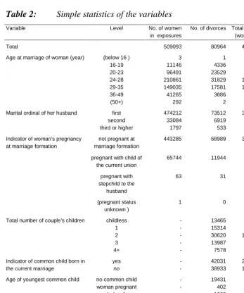
Table 2: Simple statistics of the variables Variable Level No. of women
in exposures
No. of divorces Total Exposures (woman years)
Total Occurrences (women years)
Total 509093 80964 4203373.37 41969.98
Age at marriage of woman (year) (below 16 ) 3 1 36.72 0.95 16-19 11146 4336 89444.27 2191.00 20-23 96491 23529 863785.60 12228.69 24-28 210861 31829 1784154.92 16517.38 29-35 149035 17581 1178023.85 9115.72 36-49 41265 3686 287551.69 1915.82
(50+) 292 2 376.31 0.4219
Marital ordinal of her husband first 474212 73512 3944073.31 38104.62 second 33084 6919 248820.83 3591.57 third or higher 1797 533 10479.23 273.80 Indicator of woman’s pregnancy
at marriage formation
not pregnant at marriage formation
443285 68989 3593325.23 35715.90
pregnant with child of the current union
65744 11944 609676.30 6235.01
pregnant with stepchild to the
husband
63 31 370.27 19.07
(pregnant status unknown )
1 0 1.57 0.00
childless - 13465 550499.66 6796.38 Total number of couple’s children
1 - 15314 842623.66 7984.22
2 - 30620 1771503.17 15954.86
3 - 13987 759820.35 7273.21
4+ - 7578 278926.54 3961.35
yes - 42031 2484315.25 21938.17 Indicator of common child born in
the current marriage no - 38933 1719058.12 20031.81 no common child - 19431 587486.89 9876.75 Age of youngest common child
2.2 Method
We used the following intensity regression model, to determine the risk of divorce in the first marriage:
Age at marriage is categorized into five groups, namely, 16-19, 20-23, 24-28, 29-35, and 36-49 years. We have excluded women married at age below 16 or older than 49 from calculations. Age group 24-28 is the omitted reference group. Age of the youngest common child is categorized into 5 groups, namely, below 1 year, 1-2 years, 3-5 years,
square. Sigma of variance and mean zero on with distributi normal a ity, heterogene unobserved specific captures couple the of child common youngest any of age the is marriage current in the pregnant is woman that the indicator an is ; marriage current in the children common have spouses that the indicator an is ; children premarital of types of indicators of vector a is ; marriage at pregnancy of indicator an is husband the of ordinal marital the is parenthood s ith variou children w of number total s couple’ the is woman the of marriage first at age the is estimated; be to parameters of vector a estimated; be to parameters are ; baseline the is ) ( individual for duration at divorce of intensity the is ) ( formation; marriage since duration the is where ; * * * ) ( ) ( ln 5 5 4 3 2 1 i v le); ing variab (time-vary YChildAge le); ing variab (time-vary PregMar2 le) ing variab (time-vary NewKids iable) (fixed var iable) (fixed var PregMar1 iable); (fixed var Mmord le); ing variab (time-vary Parity iable); (fixed var MarAge is
distribution with zero mean and Sigma square variance. Since the observation unit in the data set is a woman, therefore, the unobserved-heterogeneity component in the model captures woman-specific heterogeneity, as we noted above. In practice, we run first a model without unobserved heterogeneity component, we run second a model with such a term. We did not find any estimates reversed in direction. However, the likelihood ratio test shows that the second model improves significantly the model fit. We also find that after capturing woman’s specific heterogeneity, the differences among the estimates became highly distinct. As following, we will present the results obtained from running the model with unobserved heterogeneity component.
3. Findings
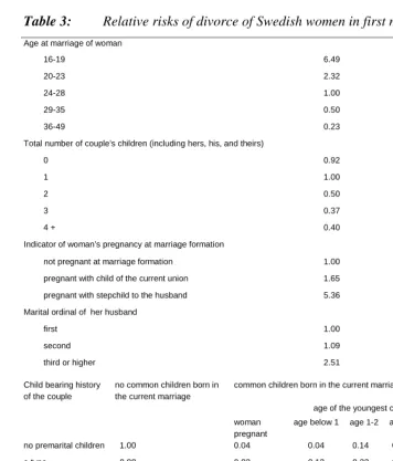
We first describe Table 3. The woman’s age at first marriage is ’only’ a control variable and, as usual, the divorce risk declines as this age increases. We also regard parity (of the couple) as a control variable. We find that, couple who remained childless or who produced only one child can be classified as one group according to the level of divorce risks. Couple who has produced two or more children can be classified as another group. The basic trend is that the divorce risk decreases as the number of children increases. The presence of the second child reduces half of the relative risk of divorce. Women who get married with a man in second marriage do not have substantially high risks of divorce, whereas, woman who marry a man in third or higher order of marriage have much higher divorce risk, compared with women who marry a man in first marriage.
As expected, women who were pregnant with a baby of the current union at the time of marriage formation had a much lower risk of divorce than that of women about to give a birth to a stepchild to her husband. Women who were not pregnant at marriage had the lowest risk of divorce. Pregnancy at marriage raised the risks of divorce regardless of the parenthood of the coming child.
Table 3: Relative risks of divorce of Swedish women in first marriages Age at marriage of woman
16-19 6.49
20-23 2.32
24-28 1.00
29-35 0.50
36-49 0.23
Total number of couple’s children (including hers, his, and theirs)
0 0.92
1 1.00
2 0.50
3 0.37
4 + 0.40
Indicator of woman’s pregnancy at marriage formation
not pregnant at marriage formation 1.00 pregnant with child of the current union 1.65 pregnant with stepchild to the husband 5.36 Marital ordinal of her husband
first 1.00
second 1.09
third or higher 2.51
Child bearing history of the couple
no common children born in the current marriage
common children born in the current marriage
age of the youngest child woman
pregnant
age below 1 age 1-2 age 3-5 age 6-8 age 9 & above
no premarital children 1.00 0.04 0.04 0.14 0.31 0.33 0.27
c-type 0.90 0.03 0.13 0.33 0.56 0.55 0.49
m-type 3.08 0.20 0.31 0.81 1.21 1.15 0.88
c-m-mixture 2.25 0.19 0.35 0.86 1.28 1.26 1.06 c-w-mixture 2.80 0.26 0.76 1.32 2.12 2.24 1.78
w-type 4.45 0.21 1.10 1.67 2.23 1.91 1.79
c-w-m-mixture 4.50 0.28 1.14 2.54 4.28 3.93 4.66 w-m-mixture 12.20 0.40 3.38 3.38 4.01 3.68 3.97
As we have noted, the lower panel of Table 3 is the result of an interaction among four covariates. One sees that the panel consists of two sets of columns, namely, (1) a single column for families with no common child born in the current marriage, and (2) a set for families with common children born in the current marriage. In the latter set, one finds the relative risks of divorce for pregnant women and for women with a youngest common child at various ages.
From the first column of the lower panel of Table 3 one finds that families with premarital children of c-type have slight lower risk of divorce. All other families show higher risks of divorce than that of childless families before the current marriage formation. This is to say, for families without childbearing after the current marriage formation, those with stepchildren to either partner have substantially higher risks of divorce than childless families do.
In the set for families with common children born in the current marriage, the relative risk displayed on the top of each column is always the smallest, except in the first column, where the second figure is the smallest. This finding implies that the existence of premarital children before the current marriage raises the subsequent divorce risk of the families where the woman is in her first marriage. Families where the couple produces a common child before the current marriage also have higher risk of divorce than that of families where there is no any premarital child. We can conclude that for families with childbearing in the current marriage, the presence of premarital children indeed lead to an excess risk of divorce independent of the parenthood of these children.
By explaining the results shown on Table 3 and Figures 1a and 1b, we describe how various compositions of a set of children born before the current marriage formation influence divorce of woman’s first marriage.
Table 3 suggests that families in which the wife had premarital children have particularly high risks of divorce. We see this from three comparisons. First, families with w-type premarital children have a higher risk of divorce than do those with m-type premarital children. Second, families with a c-w-mixture of premarital children have a much higher risk of divorce than do those with c-m-mixture premarital children. Third, families with a w-m-mixture of premarital children have a much higher risk of divorce than do those with a c-m-mixture of premarital children. This finding is so robust that it holds not only for families that do or do not have a common child in the current marriage but also for families where the wife was pregnant with the spouses’ common child at marriage. It also holds true regardless of the age of the youngest common child.
men are much less tolerant of their stepchildren than women are. Men may be more concerned about their own children. The families with premarital children of a w-m-mixture and where the couple had not produced common child after they got married had the highest risk of divorce.
Figure 1a: Divorce risks according to the age of the youngest common child, separately according to parenthood of any premarital children.
0.00 0.50 1.00 1.50 2.00 2.50 3.00 3.50 4.00 4.50 5.00 5.50
woman pregnant age below 1 age 1-2 age 3-5 age 6-8 age 9 & above
age of the youngest common child(years)
re
la
ti
ve r
isks
Figure 1b: Divorce risks according to the type of premarital children, separately according to age of the youngest common child.
Figure 1b displays the same table panel from a different angle. It confirms further what we have pointed out above. First, a woman’s pregnancy with a common child clearly reduces the risk of marriage dissolution no matter what kind of premarital children the spouses had before current marriage formation. Second, when the youngest common child was 3 years or older, the age of the youngest child no longer influenced the pattern of divorce risk; the type of premarital children then became the dominant factor shaping the curves that represent the relative risk. Third, families with common children aged 3-8 years old had the highest risk of divorce, and when the youngest common child reached 9 years or older, the divorce risk tended to decrease. But for families with premarital children of a c-w-m-mixture, the relative divorce risk reached a peak after the youngest common child reached 9 years or older. A possible reason may be that in
0.00 0.50 1.00 1.50 2.00 2.50 3.00 3.50 4.00 4.50 5.00 5.50
no premarital children
c-type m-type c-m-mixture c-w-mixture w-type c-w-m-mixture w-m-mixture
type of premarital children
relat
ive risks
risks of such families come close together. Fifth, Figure 1b also confirms that families in which the wife had premarital children who were not her husband’s have particularly high risks of divorce. The curves go up from the left to the right part of the diagram field where the relative risks for families with premarital children of c-mixture, w-type, c-w-m-mixture and w-m-mixture are displayed.
We also note that producing common children after the current marriage was formed lowered the risk of divorce for all types of families. Relative risks in Table 3 show that families where the couple did not produce common children in the current marriage had very high risks of divorce. But as the youngest common child grew, say, to age three, the families with premarital children of c-w-m-mixture experienced a higher risk of divorce. This could stem from the fact that as children grow up, tension tends to grow within the family. However, producing common could not be the cause of lowering divorce risk, instead, it could be the fact that the couple has an optimistic expectation toward their marriage and they produced subsequently a child after the marriage formation. It is equally true that the presence of a common child could serve as a tie of the family relation or somehow as an obstacle of divorce. Having common children before marriage formation cements bonds in the family. This conclusion is supported by the following facts. Families with premarital children of the c-type had the lowest risk of divorce of all families. Families with premarital children of a c-mixture had a lower risk of divorce than families with premarital children of the m-type, and families with premarital children of a c-w-mixture had a lower risk of divorce than those families with premarital children of the w-type.
In our discussion above, we have not really accounted for the fact that there is an overlap in the lower parts of Table 3 between total number of couple’s children and the type of the premarital children. For instance, if a family had premarital children of a c-w-m-mixture and the couple produced a new child in the marriage, the total number of children would be at least 4 in the family. Therefore, figures in the lower panel of Table 3 are for women of different parities. Ideally, we should make an interaction between couples’ parity and the four covariates in the lowermost of panel, but this would cause another problem--we would lose a complete combinations of premarital children with various parenthood as shown on Table 1 and Table 3. The reason is that the families with low parity, say, one or two do not have various type of premarital children (see, Liu, 2002b).
families with premarital children of the c-type, m-type and w-type. The minimum number of children of the former families is 3, but the latter types of families could have only one child. This suggests that the divorce patterns shown in Table 3 are determined mainly by the parenthood of the premarital children and the effect of premarital children seems to overwhelmingly overshadow the effect of the couple’s parity.
4. Conclusion
Families with premarital children had higher risks of divorce than families without premarital children. Having common children is always an indicator for lower divorce risks. Though, the reversed causality may exist. Premarital children from a woman’s relationship with another man made the marriage highly unstable. Premarital children to the man were much less important than premarital children to the woman. This depends probably on the fact that the women’s premarital children usually live with their mothers in the current couple’s household, whereas, men’s premarital children usually do not. The age of the youngest common child plays an additional though minor role in predicting family stability. Our findings concerning the effect of premarital children and the pattern of divorce risks in first marriages hold true even after the total number of children of the couple is controlled.
Our investigation also finds limitation of new Swedish registers. We do not know with whom the premarital children are living. We do not have information about premarital cohabitation, therefore, we can only deal with judicial marriage and do not concern union orders of both premarital cohabitation and marriages. Selection of the partner into marriages is also a disadvantage of the data we apply.
5. Acknowledgements
I thank Statistics Sweden for providing the data for this study. I am particularly grateful to Jan Hoem for his extensive substantive and editorial comments and his support throughout the whole process of this investigation. Thanks go to Jonathan MacGill, who did the programming to convert the raw data into the format needed for the aML software. I received helpful comments from Gunnar Andersson on an earlier draft of
References
Andersson, G. (1997). "The Impact of Children on Divorce Risks of Swedish Women".
European Journal of Population 13/2: 109-145.
Becker, G.S., Landes, E. M., Michael, R. T. (1977). "An Economic Analysis of Marital Instability". The Journal of Political Economy 86/6: 1141-1188.
Cherlin, A. (1978). "Remarriage as an Incomplete Institution". American Journal of
Sociology 84/3: 634-650.
Cherlin, A. J., Furstenberg, Jr., F.F. (1994). "Stepfamilies in the United States: a reconsideration". Annual Review of Sociology 20: 359-381.
Furstenberg Jr., F. F. (1990). "Divorce and the American Family". Annual Review of
Sociology 16: 379-403.
Ganong L. H. and Coleman M. (1988). "Do Mutual Children Cement Bonds in Stepfamilies?". Journal of Marriage and the Family 50: 687-699.
Hoem, J. M. (1995). "Educational Capital and Divorce Risk in Sweden in the 1970s and 1980s". Stockholm Research Reports in Demography No. 95. Stockholm University, Demography Unit.
Hong, Y. (1996). "Patterns of Divorce Risk in the 1970s and 1980s for Swedish Women with a Gymnasium Education". Stockholm Research Reports in
Demography No. 103. Stockholm University, Demography Unit.
Kravdal, Ø., 1988. "The Impact of First-Birth Timing on Divorce: new evidence from a longitudinal analysis based on the Central Population Register of Norway".
European Journal of Population 4: 247-269.
Liu, G. (2002a). "Divorce Risk of Swedish Women in Their First Marriages - two cohorts born in 1950 and 1960". Rostock, MPIDR Working Paper WP-2002-012. http://www.demogr.mpg.de/papers/working/wp-2002-012.pdf
Liu, G. (2002b). "How Premarital Children and Childbearing in the Current Marriage Influence Family Stability--descriptive findings based on Swedish register data".
Rostock, MPIDR Working Paper WP-2002-16. http://www.demogr.mpg.de/
papers/working/wp-2002-016.pdf
Qvist, J., Uhlen, M., and Sjoeberg, I. (1995). Skilsmaessor och separationer: bakgrund
Upchurch, D. M., Lillard, L. A., Panis, C. W. A. (2001). "The Impact of Non-Marital Childbearing on Subsequent Marital Formation and Dissolution". Chapter in Wu, Haveman, and Wolfe (Eds.), Out of Wedlock: Trends, Causes, and
Consequences of Nonmarital Fertility. Russell Sage, New York.