1- Introduction
The advent of micro-electro mechanical system (MEMS)-based inertial measurement units (IMUs) creates an opportunity to apply inertial navigation into a wide variety of new applications in both civil and military fields. However, the low-cost MEMS inertial sensors are affected by considerable uncertainties comprising of stochastic noises and short-term and long-term error sources [1]. Hence, the stand-alone use of MEMS IMUs in the strap-down inertial navigation system (SINS) can deliver kilometer-level positioning error after several seconds. In many applications, the SINS will be integrated with an aiding system such as global positioning system (GPS) to achieve a higher degree of accuracy.
In the SINS, the IMU measurements are provided in the body frame and the navigation parameters are calculated in the navigation frame. The measurements are transformed from the body frame to the navigation frame through direction cosine matrix (DCM). To limit the navigation error, it is very important to accurately determine the DCM matrix. The process of computing the true value of the DCM matrix is known as SINS alignment [2]. The alignment procedure contains two steps, namely, initial alignment and in-motion alignment. In the initial alignment, initialization of the SINS states will be completed prior to vehicle motion. However, due to poor initialization and cumulative IMU errors, initial alignment is insufficient to achieve the required navigation accuracy. Therefore, the SINS are often required to be re-aligned during the vehicle motion [3]. This is so-called in-motion alignment.
Regarding integrated navigation algorithms, several studies have been conducted in the literature. Using artificial neural network (ANN), Kaygisiz et al. enhanced the navigation accuracy and performance of the INS/GPS system [4]. Hao Corresponding author; Email: [email protected]
et al. presented a particle filter for SINS in-motion alignment with a large initial attitude error [5]. Wang et al. studied observability analysis for in-motion alignment of INS/GPS during different maneuvers based on perturbation model [6]. They showed that yaw-change or acceleration-change enhances the observability of misalignment angles. Stancic and Graovac proposed adaptive error damping scheme for integration of SINS and GPS [7]. A nonlinear sliding-mode observer (SMO) has been proposed for low-cost attitude-heading reference systems (AHRS) in [8]. Using infinite impulse response, (IIR) digital low-pass filter, a new algorithm for initial alignment of marine SINS has been developed in [9]. Li et al. presented a novel scheme for Doppler Velocity Log (DVL)-aided SINS alignment using unscented Kalman filter (UKF) [10]. Adaptive filtering approach has been recommended in [11] for the purpose of improving the accuracy of in-motion alignment. Musavi and Keighobadi proposed an adaptive fuzzy neuro-observer to enhance the performance of integrated INS/GPS positioning systems [12]. Magnetic calibration of strap-down magnetometers for the INS heading angle correction has been conducted in [13]. According to covariance matching techniques, adaptive unscented Kalman filter has been presented for INS/ GPS integration in [14]. Nourmohamadi and Keighobadi developed direct decentralized integration scheme for low-cost INS/GPS system in which QR-factorized cubature Kalman filter has been used as the state estimation algorithm [15].
Some researches have been dedicated to integrated navigation systems. However, there are crucial factors that may lead to some restrictions in their practical applications. For example, navigation accuracy, costs, computational cost and real-time implementation play a key role in the evaluation of navigation systems. When the navigation process runs in short time intervals, the SINS/GPS gives accurate and reliable AUT J. Model. Simul., 50(1)(2018)13-22
DOI: 10.22060/miscj.2017.12483.5036
Integration Scheme for SINS/GPS System Based on Vertical Channel Decomposition
and In-Motion Alignment
H. Nourmohammadi, J. Keighobadi*
Department of Mechanical Engineering, Tabriz University, Tabriz, Iran
ABSTRACT: Accurate alignment and vertical channel instability play an important role in the strap-down inertial navigation system (SINS), especially in the case that precise navigation has to be achieved over long periods of time. Due to poor initialization and the cumulative errors of low-cost inertial measurement units (IMUs), initial alignment is insufficient to achieve required navigation accuracy. To tackle this problem, in this paper, misalignment error is dynamically modeled and in-motion alignment is provided based on position and velocity matching. It is revealed that using misalignment error, orientation estimation can be properly corrected. Moreover, to prevent the instability effects of the vertical channel, decomposed SINS error model is derived. In the decomposed SINS error model, the navigation states in the vertical channel are separated from those in the horizontal plane. Two-step estimation process is developed for integration of the aforementioned SINS error dynamics with the measurements provided by global positioning system (GPS), and fifteen-state SINS/GPS mechanization is presented. Assessment of the proposed approach is conducted in the airborne test
Review History: Received: 3 February 2017 Revised: 9 May 2017 Accepted: 22 May 2017 Available Online: 25 July 2017 Keywords:
Low-Cost Navigation SINS/GPS Algorithm In-Motion Alignment
information. However, the accuracy of the low-cost SINS/ GPS is considerably declined with respect to the navigation time. In the practical application, in-motion alignment is very necessary to improve the long-term performance of the SINS/ GPS system. In the paper, an applied algorithm is proposed for in-run estimation of misalignment error. Accordingly, in-motion alignment is carried out simultaneously with the estimation of general navigation parameters, namely, orientation, position and velocity components. Therefore, online correction of the DCM matrix and the SINS orientation are provided. Furthermore, vertical channel instability which can impress the other navigation states in the horizontal plane is an important challenge in low-cost SINS/GPS systems. Considering this fact, in this paper, decomposed SINS error model is developed and two-step integration scheme is presented for the SINS/GPS system. In summary, the main contributions of the paper are:
• enhancing the orientation estimation accuracy in SINS/ GPS system through online estimation of misalignment error,
• developing new integration scheme based on decomposed SINS error dynamics to prevent the instability effects of the vertical channel on the overall navigation accuracy.
2- General Equations in SINS
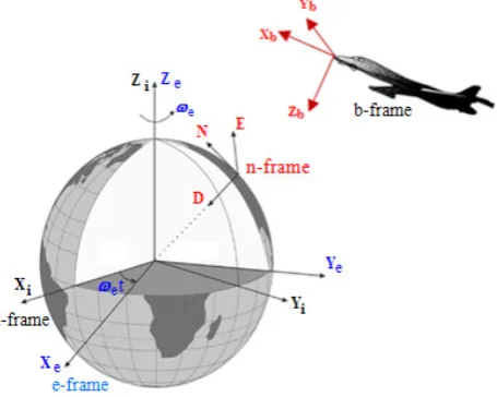
Fig.1 shows the main reference coordinate systems used in this paper, that comprises of inertial frame (i-frame), Earth-fixed frame (e-frame), navigation frame (n-frame) and body frame (b-frame). In the paper, the n-frame is the local level navigation coordinates with north-east-down (NED) geodetic axes. Basic inertial navigation equations can be divided into three parts, namely, position dynamics, velocity dynamics, and orientation dynamics.
Fig. 1. Reference coordinates frames in the inertial navigation systems [15]
Dynamics equation of the SINS position is summarized as follows.
L v
R h l
v
R h L h v
N
N
E
E D
, ( )cos , (1)
coordinates in the n-frame. RN and RE stand for meridian radii of curvature and transverse radii of curvature, respectively. The velocity equation of the SINS is expressed as follows in vector form [16].
vn C f v g
bn b ien enn n n
2 (2) where, vn is the velocity vector in the n-frame, gn is the
gravitational acceleration in the n-frame and fb is the specific force measured by the accelerometer in the b-frame. The Earth rate, n
ie
ω , and the rate of the n-frame relative to the e-frame, n
en
ω , are expressed as follows.
ien e e
T
enn
T
L L
l L L l L
cos sin
cos sin
0
(3)
where, ωe is the magnitude of the Earth rate. The orientation coordinates are defined in the paper by the roll (
ϕ
, about x-axis), pitch (θ
, about y-axis) and yaw (ψ
, about z-axis) angles known as Euler angles. Considering the sequence of z-y-x rotations, the DCM matrix between the b-frame and the n-frame is expressed as follows [17].(4)n b
C C C S S S C S S C S C
C S C C S S S S C C S S
S S C C C
θ ψ ϕ ψ ϕ θ ψ ϕ ψ ϕ θ ψ θ ψ ϕ ψ ϕ θ ψ ϕ ψ ϕ θ ψ
θ ϕ θ ϕ θ
− + +
= + − +
−
C
where, C and S denote cosine and sine functions, respectively. The orientation equation of the SINS can be expressed as in the following matrix form known as Poisson equation [18].
Cbn C
bn nbb
(5)
where, b nb
Ω is a skew-symmetric matrix representing the rate of the b-frame relative to the n-frame. In low-cost SINS, b
nb
Ω
can be approximated into b ib
Ω which is measured by the gyro in the b-frame. The equations (1), (2) and (5) are the basic SINS equations. Using these equations with the given initial states and the IMU measurements, the navigation states are estimated.
3- Sins Error Model
The main source of the navigation error in the SINS arises from the inaccurate measurements of the MEMS IMU. The accelerations measured in the b-frame are neither accurate nor are they properly transformed into the n-frame. This is due to the erroneous calculation of the orientation and the DCM matrix. Mutually, the error in the calculations of navigation states will be propagated into the calculation of rotation rates, n
ie
ω and n en
ω . The standard form of the SINS error model can be organized by three batch dynamics equations, including position error, velocity error, and misalignment error equations.
3- 1- Position Error Dynamics
The linearized position error dynamics can be obtained by perturbing the dynamics equation of the geodetic positions. The position in the n-frame is expressed by curvilinear coordinates as
[
]
TL l h
=
r . Since the position dynamics is a function of position and velocity, the linear differential equation of the position error is derived as follows.
rrr r vn
where
δ
r and δvn are the position and velocity error vectors, respectively.[
]
TT
n n n
N E D
ˆ L l h
ˆ v v v
δ δ δ δ
δ δ δ δ
= − =
= − =
r r r
v v v
(7)
Note that, (^) characterizes the estimated values. Using (1), we can rewrite (6) as follows:
L v
R h h R h v
l v L L
R h L
v h
N
N N N
E E E ( ) ( ) ( ) ( ) 2 2 1 sin
cos (( )
( )
( )
R h L
v R h L h v
E
E E
D
2cos cos
(8)
The above equation describes the position error dynamics of the SINS. Note that, the time step between the measurement updates is very small and during this short period, the assumption of linear propagation shall be taken to model the SINS error.
3- 2- Velocity Error Dynamics
Referring to (2), the estimated velocity is assumed to be propagated in accordance with:
n n b n n n n
b ˆ ie en
ˆ ˆ ˆ
ˆ ˆ ˆ
v =C f −( 2ω +ω ) v× +g (9)
The estimated DCM matrix, ˆn b
C , is written in terms of the true DCM matrix, n
b
C , and the misalignment errors as follows [16].
[
]
n n
b b
ˆ = −
C I E C (10)
where Iis an identity matrix andErepresents misalignment matrix constructed by the misalignment angles, δα, δβ and
δγ.
[ ]
0E 0 0 δγ δβ ε δγ δα δβ δα − = × = − − (11)
Perturbing (9) and, then, replacing (2) and (10), we can extract the following equation after ignoring the error product terms.
v B f µ v
v
n n n
ien enn n n
ien enn
2
2
gn (12)where fn is the specific force in the n-frame and the accelerometer error δf n has been approximated by accelerometer bias Bn. The term (2 n n)
ie en
δω +δω is obtained by calculating the first differential variation of the vector
(2 n n) ie en
ω +ω . Moreover, the following equation is considered for the gravity variation with respect to the altitude.
2 0 R g g R h = +
(13)
where g0 is the equatorial gravity and g is the gravity at
the altitude of h. The vectorδgn is obtained by the first
differential variation of (13). After some mathematical simplifications, the following equations can be derived for the velocity error dynamics.
2 2 2 2 2 2sin ( )cos 2 cos ( )cos tan ( ) ( ) D
N D E N
N
N E
e E D
E N E e E E N D E N E N v
v f f v
R h
v v
L v v
R h L R h
v
v L L
R h L
v v
v L h B
R h R h
δ δβ δγ δ ω δ δ ω δ δ = − + + − + + + + + − + + + − + + + (14)
( ) 2
2
tan 2 sin
tan 2 cos
2 cos sin
( )cos ( tan )
( )
E
E D N e N
E
D N E
E e D
E E
N E
e N D
E
E D N
E E
v L
v f f L v
R h
v v L v L v v
R h R h
v v
v L v L L
R h L
v v v L h B
R h δ δα δγ ω δ δ ω δ ω δ δ = − + + + + + + + + + + − + + + − + + (15) 2 2 2 2 2
2 cos 2 sin
2
( ) ( )
N
D E N N
N
E
e E e E
E N E D E N v
v f f v
R h
v
L v v L L
R h
v
v g h B
R h
R h R h
δ δα δβ δ ω δ ω δ δ = − + − + − + + + + + − + + + + (16)
where fN , fE and fD represent the specific force coordinates
in the n-frame and BN, BE and BD are the accelerometer
bias coordinates in the n-frame. 3- 3- Misalignment Error Dynamics
Referring to (5), we express the estimated version of the orientation dynamics in accordance with the following equation.
(
)
n n b b
b b ib in
ˆ ˆ ˆ ˆ
C =C Ω −Ω (17)
Replacing (17) in the derivative of (10) and then ignoring the error product terms results in:
(
)
n b b b
b ib in n
E= −C δΩ −δΩ C (18)
The vector form of (18) is expressed as follows by using the properties of the DCM matrix.
(
)
n b b
b ib in
ε= −C δω −δω (19)
In order to equate b in
δω , we start with ˆb ˆbˆn in n in
ω =C ω , which can be expanded into:
(
)
(
)
b b b n n
in in n in in
ω +δω =C I E+ ω +δω (20) Ignoring the error product term in (20) results in:
(
)
(
[ ]
)
b b n n b n n
in n in in n in in
δω =C δω +Eω =C δω + ×ε ω (21) Inserting (21) into (19) yields:
[ ]
n n n n n n
in in ib in in D
ε δω= + ×ε ω −δω =δω −ω ×ε− (22) Note that the gyro error has been approximated into gyro drift, Dn. The term n
in
δω is obtained by calculating the first differential variation of the vector n
in
ω . After some mathematical simplifications, the following equations are derived for the misalignment error dynamics.
. .
. .
2
2
tan sin
1
sin
( )
tan
sin cos
1
( )
tan cos
N E
e
E N
E
E e N
E E
E E
e e
E E
N
N E
N N
N E
e
N E
v
v L
L
R h R h
v
v L L h D
R h R h
v L v
L L
R h R h
v
v h D
R h R h
v L v
R h R h
δα ω δβ δγ
δ ω δ δ
δβ ω δα ω δγ
δ δ
δγ δα ω δβ
= − + + + +
+ − − −
+ +
= + + + + +
− + −
+ +
= − + − + + −
2 2
tan cos
( )cos ( )
E E
E E
e D
E E
L v
R h
v v L
L L h D
R h L R h
δ
ω δ δ
+
− + + + + −
(23)
In the above equations,DN , DE and DD represent the gyro
drift coordinates in the n-frame. 3- 4- Deriving Orientation Error
This section deals with developing a relationship between the orientation error, i.e. roll, pitch, and yaw angle error, and the misalignment error. Let us begin with the equation that relates the estimated body-to-navigation frame DCM matrix to the true one.
n n
b b
1
ˆ 1
1
δγ δβ
δγ δα
δβ δα
−
= −
−
C C (24)
The matrix n b
C is given in (4). It is assumed that (4) is held
for both estimated and true values of the DCM matrix. For the estimated one, the corresponding roll, pitch, and yaw angles are expressed in terms of their true values plus an error as follows.
ˆ
ˆ , , ˆ
ϕ ϕ δϕ= + θ θ δθ= + ψ ψ δψ= + (25) The objective is to relate the above error angles with the misalignment error. This is accomplished by selecting elements in the estimated DCM matrix, expanding them into terms of the trigonometric relationships for the sums of angles, and equating those expressions to their corresponding terms from the matrix multiplication given in (24). For example, we begin with the element (3, 1) in the matrix ˆn
b
C ,
ˆ
sinθ δβcos cosθ ψ δαcos sinθ ψ sinθ
− = − − (26)
Substituting sinθˆ with sin(θ δθ+ ) and expanding it in terms of the trigonometric relationships yield:
ˆ
sinθ=sin(θ δθ+ ) sin; θ+cosθ δθ (27)
By inserting (27) into (26), the following relationship is derived for δθ.
sin cos
δθ = ψ δα− ψ δβ (28)
Continuing in a similar procedure for elements (3, 2) and (1, 1) in the matrix ˆn
b
C results in: cos sec sin sec
tan cos tan sin
δϕ ψ θ δα ψ θ δβ
δψ θ ψ δα θ ψ δβ δγ
= − −
= − − −
(29) Therefore, the orientation error vector is calculated from the misalignment error as follows.
cos sec sin sec 0
sin cos 0
δϕ ψ θ ψ θ δα
δθ ψ ψ δβ
− −
= −
Finally, the estimated orientation is corrected by subtracting the orientation error from the estimated orientation based on (25).
3- 5- Sensor Error Model
Inertial sensor errors deteriorate the overall navigation accuracy in the SINS. Although accelerometer errors have minor effects on the SINS performance, gyro errors usually play a crucial role. These errors should be modeled stochastically and included in the SINS error model. Here, accelerometer bias and gyro drift have been considered as the inertial sensor errors. The model of IMU error is adopted under the assumption that the gyro drift can be approximated by a first-order Gauss-Markov process, and the accelerometer bias by a constant value. Therefore, the gyro drift and the accelerometer bias are modeled as follows.
i i
i
N , E, D
N , E, D
D D 2 w( t ), i
B 0 , i
β σ β
= − + =
= = (31)
where β and σ are the correlation coefficient and the standard deviation of the sensor measurement, respectively, and w t( ) is a Gaussian white noise with unity power spectral density [19].
4- Integrated SINS/GPS Navigation
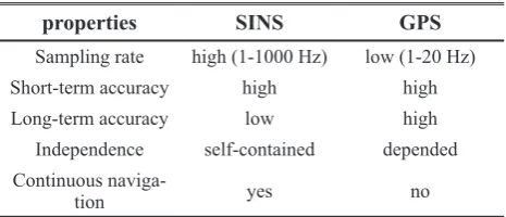
Table 1 shows a brief comparison between the SINS and the GPS characteristics. It can be obviously inferred that there are very complementary characteristics between the SINS and the GPS performance. The objective is to develop an applied mechanization for the integration between the SINS and the GPS outputs to take advantage of their characteristics.
Table 1. Comparison between the SINS and the GPS characteristics
properties SINS GPS
Sampling rate high (1-1000 Hz) low (1-20 Hz)
Short-term accuracy high high
Long-term accuracy low high
Independence self-contained depended Continuous
naviga-tion yes no
Here, considering vertical channel instability effects and in-motion alignment, a new scheme for SINS/GPS integration is developed. Misalignment error is estimated during the navigation process and in-motion alignment is achieved. Regarding vertical channel instability, decomposed error model is presented. In order to enhance the long-term performance of the integrated SINS/GPS, decomposed SINS error dynamics are applied in the filtering process instead of the standard SINS error model.
4- 1- Decomposed SINS Error Dynamics
This section deals with the vertical channel instability and its effects on the SINS performance. It can be revealed that the source of this instability is the gravity variation with respect to the altitude. The equation (32) states a typical equation for vertical channel error model (note that (32) is a simplification of (16)):
It can be inferred from the solution of (32) that the vertical channel error exponentially increases over time. In other words, the positive feedback in (32) due to the errors in the calculation of the gravity vector leads to an instability in the vertical channel. Obviously, the vertical channel instability not only affects the vertical components but also impresses on the estimation accuracy of other navigation states in the horizontal channels. In order to prevent the effect of vertical channel instability on the estimation of the other navigation states, the SINS error model is decomposed into two parts, including vertical channel and horizontal plane.
The decomposed error model of the SINS is obtained using the following state vectors.
0 0 0 1
( )
0 0 1 0
( ) ( )
0 1 0 0 0
0 0 0 0 0
0 0 0 0
E 2 E
2 2
E N
V 2 2
E N
v tan L R h
v v 2 g
R h R h R h
β − + + − = + + + − − A (36)
The linearized SINS error dynamics given in (8), (14) – (16) and (23) are derived with the assumption of neglecting the error product terms. Furthermore, the calculation of the matrices AH and AV has been done with the assumption of
neglecting the coupling terms in the SINS error model. The coupling terms are those of the vertical state vector, xV, in the
horizontal plane dynamics and those of the horizontal state vector, xH, in the vertical channel dynamics. Note that, in the
low-cost SINS/GPS system in which MEMS-grade IMU is applied to provide inertial measurements, the coupling terms between the vertical channel and the horizontal plane are negligible in comparison with the sensors’ noises, biases, and other stochastic errors.
[
]
[
]
T H
N E N E N E
T V
D D D
a v v L l B B D D v h B D
δ δβ δ δ δ δ δγ δ δ
= = x
x (33)
where xH contains the horizontal plane components and V
x contains the vertical channel components of the SINS error states. Finally, the following decomposed dynamics are defined for the SINS error model.
H H H
V V V = =
x A x
x A x (34)
The matrices AH and AV
can be obtained from the SINS error dynamics given in (8), (14) – (16), (23) and (31) as follows. (35) ( ) 2 2 tan 1
0 sin 0 sin 0 0 0 1 0
tan 1
sin 0 0 0 0 0 0 0 1
2 cos
0 2sin 0 1 0 0 0
( )cos
( )cos
2 cos sin
tan tan
0 2 sin
− − − − + + + − − + + − − − + − + + + − + + = + + E e e E E E e E N e E D E
D e E
N E
E
e N D
D N
E
H D e
E E
v L
L L
R h R h
v L
L
R h R h
v L
v v
f R h L R h L v
R h L
v L v L
v v L
v L
f L
R h R h
ω ω ω ω ω ω ω
A 2 0 0 1 0 0
( )cos
1
0 0 0 0 0 0 0 0 0
sin 1
0 0 0 ( )cos ( )cos 0 0 0 0 0
0 0 0 0 0 0 0 0 0 0
0 0 0 0 0 0 0 0 0 0
0 0 0 0 0 0 0 0 0
0 0 0 0 0 0 0 0 0
+ + + + + − − N E E N E E E v v
R h L
R h
v L
R h L R h L
β β 4- 2- Integration Scheme
In this section, fifteen-state SINS/GPS integration scheme is developed based on the decomposed SINS error dynamics. The achieved dynamical system contains fifteen states, namely, misalignment errors, velocity errors, position errors, accelerometer biases and gyro drifts. Measurement system contains GPS position, velocity, and heading angle. Based on the decomposed SINS error’s dynamics, the system differential equations in continuous-time form are given as follows.
H H H H H
V V V V V
= +
= +
x A x G u
x A x G u
(37) where G is a design matrix and u represents the system noise vector assumed to be white, Gaussian and zero-mean. Since the SINS is implemented with high-rate sampled data, (37) is transformed into its discrete-time form:
H H H H
k 1 k k k
V V V V
k 1 k k k
Φ Φ + + = + = +
x x w
x x w
(38) where Φk is the state transition matrix, and wk is the driven response at time tk+1 due to the system noise during the time
interval (tk ,tk+1). Since a white sequence is a sequence of
zero-mean random variables which are uncorrelated time-wise, the covariance matrix associated with wk is obtained as follows.
. .
[
]
k k i, i k
E
0 , i k
=
= ≠
Q
w w (39)
The state transition matrices can be calculated by the following numerical approximation.
k
k
H H H
V V V
exp( t ) I t
exp( t ) I t
Φ Φ
= ∆ ≈ + ∆
= ∆ ≈ + ∆
A A
A A
(40)
where ∆t is the sampling time. The measurement equation is defined in two parts as follows.
H H H H
k k k k
V V V V
k k k k
= +
= +
z z
H x e
H x e
(41)
where ek stands for the measurement noise with the following covariance matrix.
[
]
[
]
00k k i
k i
, i k
, i k
, i ,k
=
= ≠
= ∀
R E e e
E w e
(42)
The measurement vectors zH and zV are constructed based on the difference between the GPS and SINS outputs in calculation of position vector, velocity vector, and heading angle.
G
G G
H V G
D D G
N N
G G
E E
L L h h
l l , v v
v v
v v ψ ψ
−
−
−
= = −
−
−
−
z z (43)
The observation matrices HH and HV are obtained as follows.
0 0 0 0 1 0 0 0 0 0 0 0 0 0 0 1 0 0 0 0 0 0 1 0 0 0 0 0 0 0 0 0 0 1 0 0 0 0 0 0 H
=
H (44)
0 0 1 0 0 0 1 0 0 0 1 0 0 0 0 V
=
−
H (45)
Kalman filter is applied as the estimation algorithm for the integration of the measurement data and the dynamical system. Kalman filter is implemented in two steps known as time update and measurement update [20]. Time update is the prediction stage in which the predicted value of the state vector, xˆk−, and the error covariance,
k−
P , are provided. T
k k 1 k 1 k 1 k 1
k k 1 k 1
ˆ
Φ Φ
Φ −
− − − −
−
− −
= +
=
P P Q
x x (46)
Measurement update is the correction stage in which Kalman gain, i.e. Kk , is computed first, and then the state vector and the error covariance are updated as follows.
(
)
1T T
k k k k k k k
k k k k k k
ˆ ˆ ˆ
−
− −
− −
= +
= + z −
K P H H P H R
x x K H x (47)
In order to integrate the SINS with the GPS, two independent Kalman filters are constructed for the decomposed SINS error dynamics. Therefore, the integration in the horizontal plane is entirely separated from that of the vertical channel. Using the estimated misalignment errors, the DCM matrix can be corrected by reformulating (10) as follows.
[
]
n n
b = + ˆb
C I E C (48)
Therefore, in-motion alignment is carried out during the navigation process. The accurate orientation is obtained from the corrected DCM matrix. Using the estimated position and velocity errors, the SINS position and velocity are corrected. The main advantage of the proposed approach is that the vertical channel instability effects cannot lead to the degradation in the estimation accuracy of the navigation states in the horizontal plane. Consequently, the long-term performance of the low-cost SINS/GPS navigation will be enhanced.
5- Experimental Results and Discussion
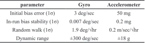
In order to assess the long-term performance of the proposed integration scheme of the low-cost SINS/GPS system, the airborne test has been conducted. MEMS-grade ADIS-16407 IMU has been used to provide the inertial measurements, that they are angular rates and specific forces. Garmin-35 GPS receiver has been used to produce the measurement data for the integrated navigation system. The main statistical specifications of the inertial sensors in ADIS-16407 IMU are given in Table 2.
Table 2. Statistical specifications of the Inertial sensors in ADIS-16407.
parameter Gyro Accelerometer
Initial bias error (1σ) 3 deg/sec 50 mg In-run bias stability (1σ) 0.007 deg/sec 0.2 mg
Random walk (1σ) 1.9 deg/√hr 0.2 m/sec/√hr Dynamic range ±300 deg/sec ±18 g
In the flight test, the proposed SINS/GPS system was installed beside a precise Vitans integrated navigation system. The highly accurate attitude data provided from Vitans system are considered as the reference values for the attitude accuracy assessment of the proposed algorithm. The raw IMU measurements are acquired at a sampling rate of 50 Hz. The SINS orientation, velocity, and position are delivered at the same rate but corrected by the GPS data at a rate of 1 Hz in the estimation filter. The error between the SINS and GPS position, velocity and heading angle are used to construct the measurement vector of the estimation algorithm. Fig. 2 represents the reference geographical latitude-longitude trajectory of the vehicle during the flight test. The test has been executed for approximately 1200 seconds along a trajectory with wide-range dynamic maneuvers. In Fig. 2, the estimated latitude-longitude trajectory of the vehicle has been compared with that of the GPS system as the true reference trajectory.
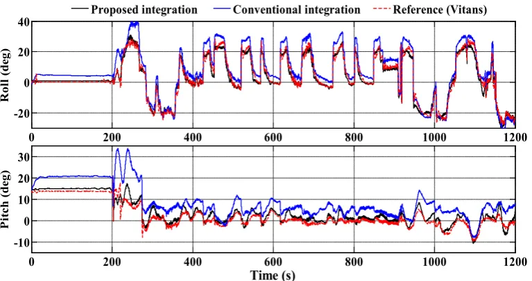
the SINS dynamics without separating the vertical channel states from those in the horizontal plane. In the conventional integration scheme, basic nonlinear dynamics of the SINS are used in the estimation process. Extended Kalman filter (EKF) is used as the state estimation filter in the integration process of the conventional integration scheme. Navigation states of the conventional integration contain position, velocity and orientation components. Unlike the proposed integration scheme, the conventional one does not use misalignment states and in-motion alignment. Figs. 3 and 4 show the estimation results of the attitude and heading angles through both the conventional and the proposed scheme. The estimated attitude has been compared with those of the accurate Vitans system and the estimated heading angle with that of the GPS system. According to Figs. 3 and 4, through the proposed integration scheme, the bias and drift terms of the MEMS-grade inertial sensors are properly compensated. The misalignment errors and the associated orientation errors are obtained appropriately. Figs. 3 and 4 depict the proposed algorithm results in a better orientation estimation in comparison with the conventional integration scheme. In Figs. 5 and 6, the estimated position and velocity are compared
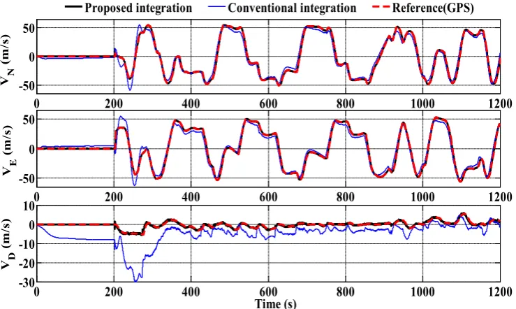
with respect to the GPS data as the reference values. Figs. 5 and 6 demonstrate the better performance of the proposed algorithm in the position and velocity estimation.
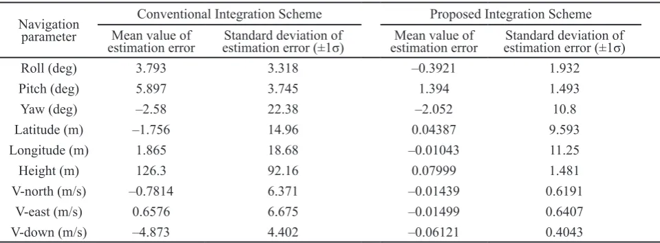
For a better evaluation, the statistical mean and standard deviation values of the estimation errors corresponding to both the conventional and the proposed integration schemes are displayed in Table 3. According to Table 3, the mean and standard deviation values of the orientation, position and velocity errors through the proposed algorithm are considerably decreased, compared to the conventional integration scheme. It can be clearly inferred from the results that using decomposed SINS error model in the estimation filter of the SINS/GPS system gathered with online compensation of misalignment errors, the navigation accuracy will be enhanced.
6- Conclusion
Due to the weak stand-alone accuracy as well as the poor run-to-run stability of the current generation of low-cost MEMS-grade IMUs, they are not applicable as a sole inertial navigation system. Moreover, the integration of such inertial unit into an aiding navigation system requires special approaches. In this paper, we focused on developing an applied approach with an appropriate long-term performance for the integration of a low-cost SINS with the GPS system. A new integration scheme was proposed for low-cost SINS/ GPS systems based on decomposed SINS error model and in-run compensation of misalignment errors. On average, the proposed algorithm reduces the mean and standard deviation of the orientation error from 4.09 deg and 9.81 deg in the conventional integration algorithm to 1.28 deg and 4.74 deg in the proposed one, respectively. Those of the position error decrease from 43.31 m and 41.93 m to 0.045 m and 7.44 m, and the velocity error from 2.10 m/s and 5.816 m/s to 0.0302 m/s and 0.535 m/s. With considering the theoretical and practical superiorities of the proposed integration scheme over traditional and conventional algorithms, it is more suitable for implementation in low-cost SINS/GPS systems, especially in aerospace application.
0 200 400 600 800 1000 1200
-20 0 20 40
Rol
l (
de
g)
0 200 400 600 800 1000 1200
-10 0 10 20 30
Time (s)
Pi
tc
h (
de
g)
Proposed integration Conventional integration Reference (Vitans)
Figure 3. Estimation results of the attitude compared with the reference value of Vitans system
34.735 34.74 34.745 34.75 34.755 34.76 34.765 34.77 34.775 34.78 50.89
50.9 50.91 50.92 50.93 50.94 50.95 50.96
Latitude (deg)
L
ong
it
ude
(
de
g)
Estimated Reference (GPS)
0 200 400 600 800 1000 1200 -200
0 200 400 600 800 1000 1200
Time (s)
Yaw (
de
g)
Proposed integration Conventional integration Reference (GPS)
Figure 4. Estimation result of the heading angle compared with the reference value of the GPS data
0 200 400 600 800 1000 1200
34.7 34.75 34.8
Lati
tu
de
(d
eg)
0 200 400 600 800 1000 1200
50.85 50.9 50.95 51
Lon
gi
tu
de
(d
eg)
0 200 400 600 800 1000 1200
500 1000 1500 2000
Time (s)
H
ei
gh
t (m)
535 540 545 34.767
34.768 34.769
852 854 856 50.94
50.942 50.944 Proposed integration Conventional integration Reference (GPS)
Figure 5. Estimation result of the position components compared with the reference value of the GPS data
0 200 400 600 800 1000 1200
-50 0 50
V N
(m/
s)
0 200 400 600 800 1000 1200
-50 0 50
V E
(m/
s)
0 200 400 600 800 1000 1200
-30 -20 -100 10
Time (s)
V D
(m/
s)
References
[1] Z. Ding, H. Cai, H. Yang, An improved multi-position calibration method for low cost micro-electro mechanical systems inertial measurement units, Proceedings of the Institution of Mechanical Engineers, Part G: Journal of Aerospace Engineering, 229(10) (2015) 1919-1930.
[2] N. El-Sheimy, S. Nassar, A. Noureldin, Wavelet de-noising for IMU alignment, IEEE Aerospace and Electronic Systems Magazine, 19(10) (2004) 32-39.
[3] J. Ali, M. Ushaq, A consistent and robust Kalman filter design for in-motion alignment of inertial navigation system, Journal of Measurement, 42(4) (2009) 577-582.
[4] B.H. Kaygisiz, I. Erkmen, A.M. Erkmen, GPS/INS enhancement for land navigation using neural network, Journal of Navigation, 57(02) (2004) 297-310.
[5] Y. Hao, Z. Xiong, Z. Hu, Particle filter for INS in-motion alignment, in: 1st IEEE Conference on Industrial Electronics and Applications, IEEE, pp. 1-6, 2006.
[6] Q. Wang, Y. Li, K. Wang, C. Rizos, S. Li, The observability analysis and SPKF for the in-motion alignment of the loosely-integrated GPS/INS system, in: Proceedings of the 22nd International Technical Meeting of The Satellite Division of the Institute of Navigation, ION GNSS, pp. 104-110, 2009.
[7] R. Stancic, S. Graovac, The integration of strap-down INS and GPS based on adaptive error damping, Robotics and Autonomous Systems, 58(10) (2010) 1117-1129.
[8] P. Doostdar, J. Keighobadi, Design and implementation of SMO for a nonlinear MIMO AHRS, Mechanical Systems and Signal Processing, 32 (2012) 94-115.
[9] Q. Li, Y. Ben, F. Sun, A novel algorithm for marine strapdown gyrocompass based on digital filter, Journal of Measurement, 46(1) (2013) 563-571.
[10] W. Li, J. Wang, L. Lu, W. Wu, A novel scheme for DVL-aided SINS in-motion alignment using UKF techniques,
Sensors, 13(1) (2013) 1046-1063.
[11] T. Liu, Q. Xu, Y. Li, Adaptive filtering design for in-motion alignment of INS, in: Control and Decision Conference (2014 CCDC), The 26th Chinese, IEEE, 2014, pp. 2669-2674.
[12] N. Musavi, J. Keighobadi, Adaptive fuzzy neuro-observer applied to low cost INS/GPS, Journal of Applied Soft Computing, 29 (2015) 82-94.
[13] H. Milanchian, J. Keighobadi, H. Nourmohammadi, Magnetic Calibration of Three-Axis Strapdown Magnetometers for Applications in Mems Attitude-Heading Reference Systems, AUT Journal of Modeling and Simulation, 47(1) (2015) 55-65.
[14] Y. Meng, S. Gao, Y. Zhong, G. Hu, A. Subic, Covariance matching based adaptive unscented Kalman filter for direct filtering in INS/GNSS integration, Journal of Acta Astronautica, 120 (2016) 171-181.
[15] H. Nourmohammadi, J. Keighobadi, Decentralized INS/GNSS System With MEMS-Grade Inertial Sensors Using QR-Factorized CKF, IEEE Sensors Journal, 17(11) (2017) 3278-3287.
[16] D. Titterton, J.L. Weston, Strapdown inertial navigation technology, IET, 2004.
[17] O.S. Salychev, Applied Inertial Navigation: problems and solutions, BMSTU Press Moscow, Russia, 2004.
[18] R.M. Rogers, Applied mathematics in integrated navigation systems, Aiaa, 2003.
[19] M. El-Diasty, S. Pagiatakis, Calibration and stochastic modelling of inertial navigation sensor errors, Journal of Global Positioning Systems, 7(2) (2008) 170-182.
[20] X.-Y. Chen, J. Yu, X.-F. Zhu, Theoretical analysis and application of Kalman filter for ultra-tight global position system/inertial navigation system integration, Transactions of the Institute of Measurement and Control, 34(5) (2011) 648-662.
Table 3. Mean values and standard deviation of the navigation error
Navigation parameter
Conventional Integration Scheme Proposed Integration Scheme Mean value of
estimation error estimation error (±1σ)Standard deviation of estimation errorMean value of estimation error (±1σ)Standard deviation of
Roll (deg) 3.793 3.318 –0.3921 1.932
Pitch (deg) 5.897 3.745 1.394 1.493
Yaw (deg) –2.58 22.38 –2.052 10.8
Latitude (m) –1.756 14.96 0.04387 9.593
Longitude (m) 1.865 18.68 –0.01043 11.25
Height (m) 126.3 92.16 0.07999 1.481
V-north (m/s) –0.7814 6.371 –0.01439 0.6191
V-east (m/s) 0.6576 6.675 –0.01499 0.6407
V-down (m/s) –4.873 4.402 –0.06121 0.4043
Please cite this article using:
H. Nourmohammadi, J. Keighobadi, Integration Scheme for SINS/GPS System Based on Vertical Channel Decomposition and In-Motion Alignment, AUT J. Model. Simul. Eng., 50(1)(2018) 13-22.