Finite Mixture Estimation Algorithm
for Arbitrary Function Approximation
Volk, M. – Nagode, M. – Fajdiga, M. Matej Volk*–Marko Nagode –Matija Fajdiga
University of Ljubljana, Faculty of Mechanical Engineering, Slovenia
The paper considers a new prospect of the arbitrary continuous function approximation from a limited set of input data with the REBMIX algorithm, developed for the finite mixture density estimation. Since the REBMIX estimates the unknown parameters with the unique semi-parametric method, it is assumed that it could be used also for the estimation of the unknown parameters in the fields that are not directly connected to density function estimation.
For the approximation of the arbitrary continuous function with the REBMIX algorithm, the required procedure is developed in the paper. The results gained by the proposed procedure and by the radial basis function network for three different datasets are compared by calculating the RMSE values between estimated and test output values. The adequacy of the proposed procedure is estimated by using both univariate and bivariate datasets. It can be concluded that with the developed procedure, the REBMIX algorithm can be applied successfully for the continuous function approximation.
Keywords: REBMIX algorithm, function approximations, finite mixtures, RBF networks, parameter estimation
0 INTRODUCTION
Since the beginning of neural networks research [1], the field of neural networks has been established as an interdisciplinary subject with deep roots in neurosciences, psychology, mathematics, the physical sciences and engineering [2] to [7]. Radial Basis Function (RBF) networks emerged as a variant of artificial neural networks in the late 1980’s. However, their roots reach further back to much older pattern recognition techniques, such as potential functions, clustering, functional approximation, spline interpolation and mixture models [8]. Until now the RBF networks have been successfully applied to a large diversity of applications including interpolation [9], classification [10], speech recognition [11], image restoration [12], 3-D object modelling [13], motion estimation and moving object segmentation [14], etc. Their excellent approximation capabilities have been studied by both, Park and Sandberg and Poggio and Girosi [15] and [16]. Because of their excellent approximation properties and simple structure, RBF networks have been chosen in the research to compare the results of the arbitrary continuous function approximation.
REBMIX, which is the acronym for the Rough and Enhanced component parameter estimation that is followed by the Bayesian classification of the remaining observations for the finite MIXture estimation, is a numerical procedure that arises from an engineering viewpoint on the mixture estimation problem. The development of the REBMIX algorithm began in the late 1990’s with the work of Nagode and
Fajdiga [17]. Since then, it has evolved gradually over the years [18] to [21] and the latest improvements in modelling both univariate and multivariate finite mixtures can be found in [22] and [23] and in modelling load spectra growth in [24]. Until now it has been noted also in other research works concerning fatigue analysis [25] to [28], modelling the expected service usage [29] and [30], etc.
The paper is structured as follows. In Section 1 the required definitions are cited. In Section 2 the results of the univariate and bivariate function estimations with the proposed procedure and RBF network are presented and compared. Finally, in Section 3 the conclusions are listed and the adequacy of the proposed procedure is discussed.
1 BASIC DEFINITIONS
1.1 Radial Basis Function Network
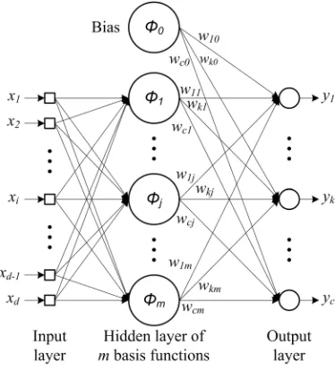
The radial basis function (RBF) network is based on the simple intuitive idea that an arbitrary function y(x) can be approximated as the linear superposition of a set of localized basis functions ϕj(x) [3]. RBF’s are
embedded in a three layer neural network shown in Fig. 1. The first layer, called the input layer is made of source nodes (sensory units) that represent the components of the input vector. The second layer, the only hidden layer in the network, consists of hidden units, which implement radial activated functions and perform a nonlinear transformation from the input space to the hidden space. The third layer, called the output layer is linear and contains units that represent a weighted sum of hidden unit outputs. Units in the output layer supply the response of the network to the activation pattern applied to the input layer and represent the components of the output vector [4].
Fig. 1. Three layer neural network
Origins of the RBF networks lie in techniques used for the exact interpolation between data points in high dimensional spaces. In applications of
neural networks, a general interest is not an exact interpolation since it can lead to particularly poor results when the trained network is presented with new data. Generally, a smooth approximation [31], which can be achieved by using fewer basis functions
m than data points n and by minimizing a
sum-of-squares error (SSE) function, can lead to much better results [2].
When m < n, the RBF neural network corresponds to a set of functions given by [2] and [3]:
yk m wkj j j
j m
(x , , )w ΘΘ = (xθθ ).
=
∑
φ0 (1)
Here wkj represents the weight of the jth basis
function output which contributes to the kth network
output yk and φj(xθθj) represents the activation of
hidden unit j when the network is presented with
d-dimensional input vector x, see Fig. 1. A bias for the output units is included in Eq. (1) as an extra “basis function” ϕ0 whose activation is fixed to be ϕ0 = 1. For
most applications the basis functions are chosen to be Gaussian:
φ
σ
j j j
j
j a
(xθθ )= ⋅exp− x−µµ ,
2
2
2 (2)
where aj controls the height of the peak, vector μj
represents the center and the parameter σj represents
the width of the jth basis function. Note that each
basis function can have its own width parameter σj
[2] and [3]. To compare the estimated values with the target values, an error function has to be used. The most commonly used form of the error function for regression problems is the SSE function [2] and [32], given by:
E ykq q m t
kq k
c
q n
=
{
(
)
−}
= =
∑
∑
1 2
2
1 1
x , ,wΘΘ , (3)
where xq denotes the qthd-dimensional input training
vector and w the output layer weight vector for current basis functions parameters Θ, tkq is the kth target
value in qth c-dimensional target vector tq. Bishop
[2] suggests assessing the performance of the trained network using different error function from that used to train them. If the SSE function is used in the network training phase, the root-mean-square error
(RMSE) function should be used in network testing.
E
y m t
t t RMS k q q kq k c q n kq k c q n =
(
)
−{
}
−{
}
= = = =∑
∑
∑
∑
x * , ,w *
* * * * Θ Θ 2 1 1 2 1 1
,, (4)
where xq* denotes the qth input test vector and n* is
the number of input test vectors, w and Θ denote the weight vector and the basis functions parameters of the trained network respectively and tkq* is the kth
target test value in the qth c-dimensional target test
vector tq*. In Eq. (4), the t* stands for the average of
the target test values:
t
n c tkq k c q n * * *. * = = =
∑
∑
1 11 (5)
Training of the RBF networks takes place in two successive stages. First, the centers and the basis function widths are determined. In the second stage the linear output layer weights are determined. For the determination of the basis functions parameters there exists a variety of procedures [2] to [4] and [33]. Since the scope of the paper is not searching for the optimal learning procedure of the RBF networks but assessing the suitability of the REBMIX algorithm for arbitrary function approximation, only simple and fast procedures for the determination of basis functions centers and width are selected in the paper, which in spite of their simplicity assure adequate network training.
The first and simplest approach to determine the basis functions centers, denoted by C1, is to set them on the highest output values in the training dataset [3]. This approach usually results in a large number of basis functions to achieve satisfactory results. The second approach for center determination, denoted by C2, is to select them randomly from the training dataset [3]. In this very commonly used learning technique the estimated function is much smoother and usually better approximates the training data with a fewer number of basis functions. The disadvantage of this approach is the reproduction of network training.
The widths of Gaussian basis functions are also determined by using two simple approaches. In the first approach, denoted by S1, the basis function widths are set to be equal to the average Euclidean distance between the adjacent basis function centers, which ensures that the basis functions overlap to some degree and hence give a relatively smooth approximation [2] and [3]. In the second approach, denoted by S2, the widths are no longer equal for all
basis functions, but are determined on the basis of the average Euclidean distance to the p-nearest centers [2] and [3].
The output layer weights are calculated in a way
to minimize the SSE function with respect to these
weights. With the insertion of Eq. (1) into Eq. (3) and the differentiation of the SEE function it is possible to rewrite the equation in matrix notation in the following form [2] and [3]:
ΦTΦWT = ΦTT, (6)
where ( )T qk =tkq and ( )ΦΦqj =φj(xq θθj). The formal
solution for the weights is given by:
WT = Φ†T, (7)
where the notation Φ† denotes the pseudo-inverse of Φ given by:
Φ† ≡ (ΦTΦ)-1ΦT. (8)
1.2 REBMIX Algorithm for the Finite Mixture Estimation
Let x1, ..., xn be an observed d-dimensional dataset
of size n of continuous vector observations xq. Each
observation is assumed to follow predictive mixture density [34]:
f m w fj j j
j m
(x , , )wΘΘ = (xθθ ),
=
∑
1
(9)
with conditionally independent component densities:
fj j f xj i ij i
d
(xθθ )= ( θθ ),
=
∏
1
(10)
indexed by vector parameter θj. The objective of the
analysis is the inference about the unknowns: the number
m of components, component weights wj summing to 1
and component parameters θj.
Since the description of the REBMIX algorithm estimation procedure and proof of its convergence is extensive and published in [17] to [24], further details will not be presented here. For interested readers REBMIX software is available at http://CRAN.R-project.org/package=rebmix.
1.3 Arbitrary Function Approximation with the REBMIX Algorithm
The first difference is related to the component weights. In the REBMIX algorithm the weights are limited with two conditions,
wj > 0 for (j = 1, ..., m) and j wj
m =
=
∑
1 1, while inthe RBF network approach there are no limitations concerning the weights for regression problems. In fact, output layer weights can also be negative. This property can be very useful for better estimation of the function valleys and for observations with negative output values. The observations with negative output values can be processed with the REBMIX algorithm only if they are previously properly treated so that all the observed values have positive signs.
The second major difference is related to the function estimation. When using the RBF network, the arbitrary function can be estimated directly from the set of observed data and therefore it usually does not integrate to unity. With the REBMIX algorithm, the arbitrary function can be approximated indirectly from the estimation of the finite mixture density, which integrates to unity,
∫
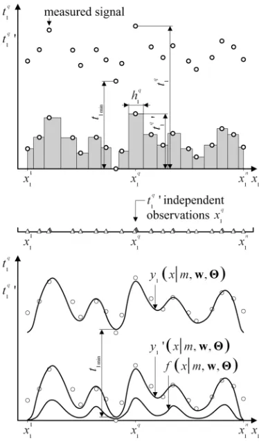
f(xm, , )w ΘΘdx=1. Therefore it is necessary to properly transform the measured training dataset and postprocess estimated finite mixture density f(xm, , )w ΘΘ in such a way that it can be compared to the observed output values.The procedure for the preparation of the observations and postprocessing of estimated function
f(xm, , )wΘΘ is depicted in Fig. 2 relying on the steps to follow:
1. All the data are either raised if tk min < 0 or
lowered for the minimal output value:
tkq'= −tkq tkmin q=1,..., ,n (11)
as it turned out that in such cases the REBMIX algorithm estimates the finite mixture density function much better. To improve the accuracy of the estimated function, tkq' may be multiplied by
a factor 10, 100, etc. and rounded to the nearest integer.
2. The volume under the shifted data is calculated by:
V tkq h iq i
d
q n
=
=
=
∏
∑
' ,1
1 (12)
where hiq is the length of the hypersquare side
for the qth data in the ith dimension.
3. The measured training dataset is transformed in such a way that REBMIX preprocessing methods can be used. With this purpose each d-dimensional input data vector xq is copied tkq' times so that
the total number of vector observations used as input data for the finite mixture estimation equals
tkq q
n
'
=
∑
1 .
4. Finite mixture estimation with the REBMIX algorithm is performed.
5. The postprocessing of the estimated finite mixture density function is carried out in such a way that the continuous function, representing input-output mapping of the original dataset is gained. Estimated finite mixture density function
f(xm, , )w ΘΘ is multiplied by the volume (12) and the transformation function is gained:
yk'(xm, , )w ΘΘ = f(xm, , ) .wΘΘV (13)
In the case of a univariate dataset, the volume reduces to the area under the observed data. The estimated function yk'(xm, , )w ΘΘ can be
compared to the true one and to the function estimated by the RBF network.
6. To compare the estimated values to the actual measured output ones, it is necessary to shift the estimated function yk'(xm, , )wΘΘ
yk'(xm, , )w ΘΘ for the minimal output value: yk(xm, , )wΘΘ =yk'(xm, , )w ΘΘ +tkmin. (14)
The correctness of the proposed procedure for the function approximation is proved by the following examples.
2 EXAMPLES
2.1 Vertical Wheel Forces Dataset
The univariate dataset used in the research derives from measurements of vertical wheel forces that occur when driving the vehicle on a test track. The entire signal, measured with 250 Hz sample rate, is shown in Fig. 3. From all measured data only a section indicated with a square containing 1070 successive data is selected for further treatment due to the faster estimation process. Approximately 30% from these data are randomly selected to form the test dataset that is used only for the evaluation of the estimated functions and is not present in the training phase when the number of components, their parameters and weights are estimated. The test dataset thus consists of n* = 320 data and the remaining n = 750 data form the training dataset.
When the RBF network is applied for the estimation of the function parameters and weights, no special preparation of the training dataset is necessary. Nevertheless, all the data used in the research are lowered for tk min to reduce the estimation
error especially on the edges of the observed function. For all combinations of the selected learning procedures C1-S1, S1, C1-S2 and C2-S2 and for each m∈
{
1,...,n}
, the basis functions parameters and weights are determined. Eachyk’(x|m,w,Θ) is then raised by tk min, the trained
RBF network yk (x|m,w,Θ) is subjected to the test
dataset and the RMSE is calculated. The network
training is stopped if RMSE≤RMSE lim, where the
RMSElim∈{0.5, 0.3, 0.2, 0.1 and min
}
or m=n.Fig. 3. Measured vertical wheel forces
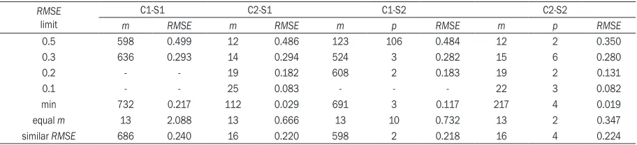
The results are shown in Table 1. In most cases the best learning combination turns out to be C2-S2. It results in the smallest number of basis functions and
the lowest RMSE, while C1-S1 stands for the worst
learning combination possible.
On the other hand, when the REBMIX is applied, all training data are lowered by tk min and the input
training data points xq are copied tq' times. Although the
REBMIX allows the selection of different preprocessing, the histogram and Parzen window are only suitable. The former is chosen in the article. For the finite mixture density, the normal parametric family is chosen. To determine optimal number of components m, parameters
Θ and weights w, finite mixture estimation is carried out for s∈
{
10,...,750}
.Thus all possible arrangements of observations are captured and the optimal number of bins is obtained according to both, the information criterion and the positive relative deviation D. Estimations are carried out for all combinations of the available information criteria
Table 1. The results of function estimation for vertical wheel forces dataset with the RBF network; the - indicates that network training is stopped before the limiting RMSE value is reached
RMSE
limit
C1-S1 C2-S1 C1-S2 C2-S2
m RMSE m RMSE m p RMSE m p RMSE
0.5 598 0.499 12 0.486 123 106 0.484 12 2 0.350
0.3 636 0.293 14 0.294 524 3 0.282 15 6 0.280
0.2 - - 19 0.182 608 2 0.183 19 2 0.131
0.1 - - 25 0.083 - - - 22 3 0.082
min 732 0.217 112 0.029 691 3 0.117 217 4 0.019
equal m 13 2.088 13 0.666 13 10 0.732 13 2 0.347
and six different D values. The estimated finite mixtures are postprocessed according to Eqs. (13) and (14) and the corresponding RMSE values are calculated. The calculated
RMSE values are than used in the continuation for the performance comparison of the proposed procedure with the RBF network.
The results are shown in Table 2. The optimal number of components increases with the decrease of
D and stops to increase if D < 0.0005. If D < 0.001, the optimal number of components increases rapidly
while there is only a small decrease of RMSE. The
mixture of 13 components is thus supposed to be the optimal one.
Table 2. The results of function estimation for vertical wheel forces dataset with the REBMIX
D m s information criterion RMSE
0.025 5 61 MDL5 0.522
0.01 7 75 AIC 0.428
0.005 12 125 AIC 0.329
0.001 13 151 MDL2 0.240
0.0005 28 116 AIC 0.211
0.0001 28 116 AIC 0.211
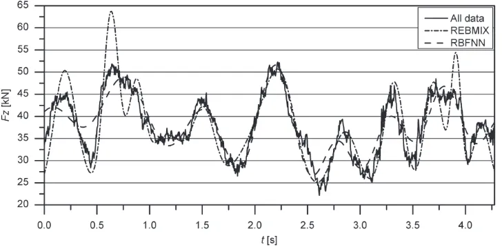
It can be noted that the RBF network requires 16 basis functions for similar RMSE as the REBMIX (see the last row in Table 1). The corresponding functions are shown in Fig. 4. Both, the RBF network and REBMIX represent the middle section well, while larger deviations appear at the edges.
2.1 Two-Dimensional Gaussian Dataset
The bivariate dataset, derived from a mixture of four Gaussian functions Bors and Pitas [33], is studied next. From a mixture of four two-dimensional (2D) Gaussian functions with the following vector parameters:
θ1 =[a1 =5, μ11 =5, μ21 =15, σ11 =2, σ21 =2], θ2 =[a2 =5, μ12 =5, μ22 =15, σ12 =5, σ22 =2], θ3 =[a3 =5, μ13 =5, μ23 =6, σ13 =3, σ23 =5] and θ4 =[a4 =5, μ14 =5, μ24 =6, σ14 =4, σ24 =2]
the 441 data yq are generated for x1∈
{
0,...,20}
and x2∈{
0,...,20}
among which n*=132 randomlyselected data form the test dataset and the residual
n=309 data form the training dataset. In addition to the noise free bivariate dataset, the random Gaussian noise with μ=0 and σ = 0.6 is added to yq to simulate
the noisy dataset, which is usually observed in the measurements.
When the RBF network is applied, no preparation of the training dataset is carried out as tk min =0.
For network training each m∈
{
1,...,n}
and allcombinations of the selected learning procedures C1-S1, C2-C1-S1, C1-S2 and C2-S2 are used. Each trained RBF network yk (x|m,w,Θ) is subjected to the test
dataset and the RMSE is calculated. The network
training is stopped if RMSE≤RMSE lim , where
RMSElim∈
{
0.5, 0.3, 0.2, 0.1 and min}
or m=n. The results are shown in Tables 3 and 4 for noise free and noisy dataset, respectively. The smallestnumber of basis functions and the lowest RMSE are
gained when the learning combinations C2-S1 and C2-S2 are applied. The worst learning combination turned out to be the C1-S1.
When the REBMIX is applied, all input training data vectors xq are only copied tq' times as tk min =0. The
histogram preprocessing and the normal parametric family are used. To determine optimal number of components m, parameters Θ and weights w, finite mixture estimation is carried out for s∈
{
1 30,...,}
in both dimensions so that all possible arrangements of observations are captured. The estimations are carried out for all combinations of the available information criteria and six different D values. The estimated finite mixtures are postprocessed according to (13) and (14), where yk (x|m,w,Θ) = yk'(x|m,w,Θ) and thecorresponding RMSE values are calculated.
The results are shown in Tables 5 and 6. For the noise free dataset the optimal number of components is the same for all D values, whereas for the noisy dataset the optimal number of components increases
by one when D≤0.01.
Table 5. The results of function estimation for the noise free bivariate dataset with the REBMIX
D m s information criterion RMSE
0.025 5 22 AIC 0.277
0.01 5 22 AIC 0.277
0.005 5 22 AIC 0.277
0.001 5 22 AIC 0.277
0.0005 5 22 AIC 0.277
0.0001 5 22 AIC 0.277
With the increase of the number of components
the RMSE value also increases. This means that
the estimated function with a larger number of components overfits the data and consequently results in a worse estimate. The mixture of 5 components is thus supposed to be the optimal one. Unlike for the
univariate dataset, where optimal sn, for the
presented bivariate datasets the optimal s>n in both dimensions. This indicates that some of the histogram bins stay empty after the observations are arranged.
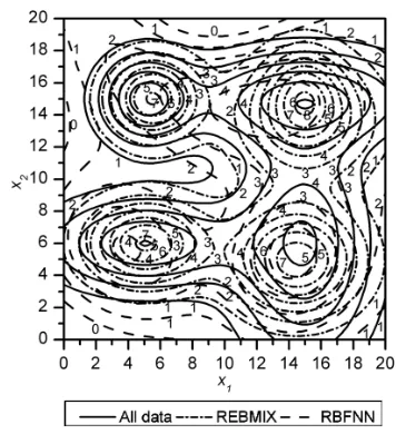
Fig. 5. Comparison between simulated noise free bivariate function and both estimated functions with similar RMSE value Table 3. The results of function estimation for the noise free bivariate dataset with the RBF network
RMSE
limit m C1-S1RMSE m C2-S1RMSE m C1-S2p RMSE m C2-S2p RMSE
0.5 31 0.487 8 0.383 7 1 0.451 8 1 0.484
0.3 65 0.296 14 0.288 16 4 0.295 13 2 0.265
0.2 76 0.194 16 0.197 19 4 0.183 19 9 0.196
0.1 118 0.100 20 0.077 35 6 0.089 23 3 0.071
min 260 1.26E-02 301 1.25E-02 120 20 5.22E-04 120 13 5.17E-04
equal m 5 0.792 5 0.615 5 4 0.738 5 2 0.534
similar RMSE 68 0.273 14 0.288 17 4 0.273 13 2 0.265
Table 4. The results of function estimation for the noisy bivariate dataset with the RBF network
RMSE
limit
C1-S1 C2-S1 C1-S2 C2-S2
m RMSE m RMSE m p RMSE m p RMSE
0.5 42 0.481 11 0.485 9 7 0.430 7 2 0.500
0.3 65 0.298 16 0.144 17 4 0.253 14 4 0.288
0.2 77 0.197 16 0.144 24 6 0.175 19 6 0.159
0.1 127 0.095 22 0.090 31 6 0.097 26 5 0.084
min 209 6.79E-02 50 3.41E-02 97 28 2.67E-02 55 4 2.54E-02
equal m 5 0.810 5 0.590 5 4 0.760 5 1 0.585
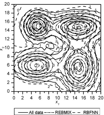
Fig. 6. Comparison between simulated noisy bivariate function and both estimated functions with similar RMSE value
The RBF network requires 13 basis functions in the case of noise free dataset and 17 basis functions in the case of noisy dataset for similar RMSE as the REBMIX (see the last row in Tables 3 and 4). The corresponding functions are shown in Figs. 5 and 6.
Table 6. The results of function estimation for the noisy bivariate dataset with the REBMIX
D m s information criterion RMSE
0.025 5 22 AIC 0.260
0.01 6 22 AIC 0.316
0.005 6 22 AIC 0.316
0.001 6 22 AIC3 0.316
0.0005 6 22 AIC3 0.316
0.0001 6 22 AIC3 0.316
In the case of the noise free dataset the function estimated by the REBMIX overestimates all four components on their peak values and slightly underestimates the simulated function in the valleys. If the analogy with the univariate function estimation is taken, it is expected that the REBMIX would estimate the underlying function even better if it was composed of a greater number of intermediate components. On the other hand, the function estimated by the RBF network underestimates the first component considerably and the second and fourth component slightly but estimates the valley between the second and the third component well. Similar results are also obtained in the case of the noisy dataset where the function estimated by the REBMIX again overestimates the peak values of all four components and slightly underestimates the valleys between them
(see Fig. 6). The function estimated by RBF network represents the first three components very well and underestimates the fourth one.
3 CONCLUSION AND FUTURE WORK
In the article continuous functions are estimated with the REBMIX algorithm for the first time. Both univariate and bivariate datasets are used to evaluate its adequacy. The estimated functions are compared to the functions estimated by the elementary RBF network.
For the applied univariate and bivariate datasets it can be concluded that the functions estimated by the REBMIX using the proposed procedure approximate the actual functions well. Hence the assumption is derived that the REBMIX can be applied for the estimation of the univariate and bivariate continuous functions if the training dataset is transformed properly and the estimated finite mixture densities are postprocessed properly. Although the procedure requires the transformation of the training data and postprocessing of the estimated function, the estimation times are still very short since all the properties of the REBMIX are preserved.
The future development of the REBMIX will be focused on its connection to the RBF networks. Possibly, the REBMIX can be used to determine the centers of basis functions μj and widths σj in the
first stage of the RBF network learning process. The determination of the final layer weights should remain unchanged. In this way the postprocessing of the estimated finite mixture density can be omitted since the estimated function would already approximate the actual observed function. The entire estimation process can also be simplified if the transformation of the training data was comprehended in the REBMIX preprocessing.
4 REFERENCES
[1] McCulloch, W.S., Pitts, W. (1943). A logical calculus of the ideas immanent in nervous activity. Bulletin of Mathematical Biophysics, vol. 5, no. 4, p. 115-133, DOI:10.1007/BF02478259.
[2] Bishop, C.M. (1995). Neural Networks for Pattern Recognition. Oxford Clarendon Press.
[3] Bishop, C.M. (1994). Neural networks and their applications. Review of Scientific Instruments, vol. 65, no. 6, p. 1803-1832, DOI:10.1063/1.1144830.
[4] Haykin, S. (1999). Neural Networks: A Comprehensive Foundation. Prentice-Hall New Jersey.
[5] Gonçalves V.D., De Almeida, L.F., Mathias, M.H. (2010). Wear particle classifier system based on an artificial neural network. Strojniški vestnik – Journal of Mechanical Engineering, vol. 56, no. 4, p. 284-288. [6] Ibrikçi, T., Saçma, S., Yıldırım, V., Koca, T. (2010).
Application of artificial neural networks in the prediction of critical buckling loads of helical compression springs. Strojniški vestnik – Journal of Mechanical Engineering, vol. 56, no. 6, p. 409-417. [7] Čas, J., Škorc, G., Šafarič, R. (2010). Improved
micropositioning of 2 DOF stage by using the neural network compensation of plant nonlinearities. Strojniški vestnik – Journal of Mechanical Engineering, vol. 56, no. 10, p. 599-608.
[8] Tou, J.T., Gonzales, R.C. (1977). Pattern Recognition Principles. Addison-Wesley Massachusetts.
[9] Broomhead, D.S., Lowe, D. (1988). Multivariable functional interpolation and adaptive networks.
Complex Systems, vol. 2, no. 3, p. 321-355.
[10] Zhang, R., Huang, G.B., Sundararajan, N., Saratchandran, P. (2007). Improved GAP-RBF network for classification problems. Neurocomputing, vol. 70, no. 16-18, p. 3011-3018, DOI:10.1016/j. neucom.2006.07.016.
[11] Bors, A.G., Gabbouj, G. (1994). Minimal topology for a radial basis function neural network for pattern classification. Digital Signal Processing, vol. 4, no. 3, p. 173-188, DOI:10.1006/dspr.1994.1016.
[12] Cha, I., Kassam, S.A. (1996). RBFN restoration of
nonlinearly degraded images. IEEE Transactions
on Image Processing, vol. 5, no. 6, p. 964-975,
DOI:10.1109/83.503912.
[13] Bors, A.G., Pitas, I. (1999). Object classification in 3-D images using alpha-trimmed mean radial basis function network. IEEE Transactions on Image Processing, vol. 8, no. 12, p. 1744-1756, DOI:10.1109/83.806620. [14] Bors, A.G., Pitas, I. (1998). Optical flow estimation
and moving object segmentation based on median radial basis function network. IEEE Transactions
on Image Processing, vol. 7, no. 5, p. 693-702,
DOI:10.1109/83.668026.
[15] Park, J., Sandberg, J.W. (1991). Universal approximation using radial basis function networks.
Neural Computation, vol. 3, no. 2, p. 246-257,
DOI:10.1162/neco.1991.3.2.246.
[16] Poggio, T., Girosi, F. (1990). Networks for approximation and learning. Proceedings of the IEEE, vol. 78, no. 9, p. 1481-1497, DOI:10.1109/5.58326. [17] Nagode, M., Fajdiga, M. (1998). A general
multi-modal probability density function suitable for the rainflow ranges of stationary random processes.
International Journal of Fatigue, vol. 20, no. 3, p. 211-223, DOI:10.1016/S0142-1123(97)00106-0.
[18] Nagode, M., Fajdiga, M. (1999). The influence of variable operating conditions upon the general multi-modal Weibull distribution. Reliability Engineering & System Safety, vol. 64, no. 3, p. 383-389, DOI:10.1016/ S0951-8320(98)00085-4.
[19] Nagode, M., Fajdiga, M. (2000). An improved algorithm for parameter estimation suitable for mixed Weibull distributions. International Journal of Fatigue, vol. 22, no. 1, p. 75-80, DOI:10.1016/S0142-1123(99)00112-7.
[20] Nagode, M., Klemenc, J., Fajdiga, M. (2001).
Parametric modelling and scatter prediction of rainflow matrices. International Journal of Fatigue, vol. 23, no. 6, p. 525-532, DOI:10.1016/S0142-1123(01)00007-X. [21] Nagode, M., Fajdiga, M. (2006). An alternative
perspective on the mixture estimation problem.
Reliability Engineering & System Safety, vol. 91, no. 4, p. 388-397, DOI:10.1016/j.ress.2005.02.005.
[22] Nagode, M., Fajdiga, M. (2011). The REBMIX algorithm and the univariate finite mixture estimation. Communications in Statistics -
Theory and Methods, vol. 40, no. 5, p. 876-892,
DOI:10.1080/03610920903480890.
[23] Nagode, M., Fajdiga, M. (2011). The REBMIX algorithm for the multivariate finite mixture estimation. Communications in Statistics - Theory
and Methods, vol. 40, no. 11, p. 2022-2034,
DOI:10.1080/03610921003725788.
[24] Volk, M., Fajdiga, M., Nagode, M. (2009). Load spectra growth modelling and extrapolation with REBMIX. Structural Engineering and Mechanics, vol. 33, no. 5, p. 589-605.
[25] Tovo, R. (2001). On the fatigue reliability evaluation of structural components under service loading.
International Journal of Fatigue, vol. 23, no. 7, p. 587-598, DOI:10.1016/S0142-1123(01)00021-4.
[26] Tovo, R. (2002). Cycle distribution and fatigue damage under broad-band random loading. International Journal of Fatigue, vol. 24, no. 11, p. 1137-1147, DOI:10.1016/S0142-1123(02)00032-4.
[27] Liu, Y., Liu, L., Stratman, B., Mahadevan, S. (2008). Multiaxial fatigue reliability analysis of railroad wheels. Reliability Engineering & System Safety, vol. 93, no. 3, p. 456-467, DOI:10.1016/j.ress.2006.12.021. [28] Ni, Y.Q., Ye, X.W., Ko, J.M. (2010).
Monitoring-Based fatigue reliability assessment of steel bridges: Analitical model and application. Journal of Structural
Engineering, vol. 136, no. 12, p. 1563-1573,
[29] Socie, D. (2001). Modelling expected service usage from short-term loading measurements. International Journal of Materials & Product Technology, vol. 16, no. 4-5, p. 295-303, DOI:10.1504/IJMPT.2001.001272. [30] Iranpour, M., Taheri, F., Vandiver, J.K. (2008).
Structural life assessment of oil and gas risers under vortex-induced vibration. Marine Structures, vol. 21, no. 4, p. 353-373, DOI:10.1016/j. marstruc.2008.02.002.
[31] Grešovnik, I. (2007). The use of moving least squares for a smooth approximation of sampled data. Strojniški vestnik – Journal of Mechanical Engineering, vol. 53, no. 9, p. 582-598.
[32] Šimunović, G., Šarić, T., Lujić, R. (2008). Application
of neural networks in evaluation of technological time. Strojniški vestnik – Journal of Mechanical Engineering, vol. 54, no. 3, p. 179-188.
[33] Bors, A., Pitas, I. (1996). Median radial basis function neural network. IEEE Transactions on
Neural Networks, vol. 7, no. 6, p. 1351-1364,
DOI:10.1109/72.548164.